Munich Personal RePEc Archive
Varying Coefficient Panel Data Model in
the Presence of Endogenous Selectivity
and Fixed Effects
Malikov, Emir and Kumbhakar, Subal C. and Sun, Yiguo
Department of Economics, State University of New York at
Binghamton, NY, Department of Economics, State University of
New York at Binghamton, NY, Department of Economics and
Finance, University of Guelph, Guelph, ON
2013
Online at
https://mpra.ub.uni-muenchen.de/55993/
Varying Coefficient Panel Data Model in the Presence of
Endogenous Selectivity and Fixed Effects
Emir Malikov∗ Subal C. Kumbhakar† Yiguo Sun‡
This Draft: November 20, 2013
Abstract
This paper considers a flexible panel data sample selection model in which (i) the outcome equation is permitted to take a semiparametric, varying coefficient form to capture potential parameter heterogeneity in the relationship of interest, (ii) both the outcome and (paramet-ric) selection equations contain unobserved fixed effects and (iii) selection is generalized to a polychotomous case. We propose a two-stage estimator. Given consistent parameter estimates from the selection equation obtained in the first stage, we estimate the semiparametric outcome equation using data for the observed individuals whose likelihood of being selected into the sam-ple stays approximately the same over time. The selection bias term is then “asymptotically” removed from the equation along with fixed effects using kernel-based weights. The proposed estimator is consistent and asymptotically normal. We first investigate the finite sample prop-erties of the estimator in a small Monte Carlo study and then apply it to study production technologies of U.S. retail credit unions from 2002 to 2006.
Keywords: Credit Union, Fixed Effects, Selection, Semiparametric, Smooth Coefficient, Switch-ing Regression, VarySwitch-ing Coefficient
JEL Classification: C14, C33, C34, G21
1
Introduction
Semiparametric methods have become a part of a standard methodological toolkit of applied re-searchers in economics. These methods are attractive for their ability to circumvent limitations of conventional parametric models by allowing more flexible specifications and thus mitigating (at least partly) the risk of misspecification. While they admittedly require more prior assumptions and therefore are not as flexible as their (completely) nonparametric counterparts, semiparametric models have nevertheless gained popularity due to their capability to alleviate the so-called “curse of dimensionality” associated with nonparametric estimation.
This paper considers a particular class of semiparametric models in which parameters of a linear regression are permitted to be unspecified smooth functions of some variables (Hastie and Tibshirani, 1993; Cai et al., 2000; Li et al., 2002). Such “varying coefficient” (hereinafter VC) models1 have recently become a subject of prolific research in the econometric literature that attempts to extend the method to new settings. For instance, Das (2005), Cai et al. (2006) and Cai and Xiong (2012) consider VC models in the presence of endogenous variables and propose applying instrumental variables approach to tackle the endogeneity problem. However, the overwhelming majority of these studies place the model either in the cross-sectional (as in the above cited papers) or in the time series settings (e.g., Cai, 2007). Analysis of VC models in a panel data setting is however relatively scarce, arguably due to difficulties associated with tackling unobserved effects. For instance, Cai and Li (2008) study a VC model in the dynamic panel setting that assumes any unobserved effects away. Sun et al. (2009) somewhat fill the void by proposing a VC panel data model estimator which allows treatment of both random and fixed effects.2
However, the semiparametric literature has broadly overlooked another important feature of the data that applied researchers often have to deal with: namely, the presence of selectivity. Such a problem is acute in studies of wage and labor supply decisions that go back to Heckman’s (1974, 1979) seminal work and many other labor economics applications and not only. In this paper, we therefore take a semiparametric VC model a step further by considering it in the panel data setting and the presence of endogenous selection and fixed effects.3 For a similar model in a cross-sectional setting, see Das et al. (2003), whose model allows both the outcome and selection equations to take completely nonparametric forms. Das (2004) extends the above model to a panel data case with (exogenous) random effects.
Thus, we consider a flexible panel data sample selection model in which (i) the outcome equation is permitted to take a semiparametric VC form to capture potential parameter heterogeneity in the relationship of interest, (ii) both the outcome and selection equations contain unobserved fixed ef-fects and (iii) selection is generalized to a polychotomous case. In this paper, we restrict our analysis to models with parametric selection equations. Our model can be considered as a generalization of conventional parametric panel data sample selection models [see Baltagi (2013) for a compre-hensive review]. Relatively few such parametric models allow for a fixed-effect type heterogeneity. For instance, in the case of strictly exogenous right-hand-side covariates, Wooldridge (1995) and
1Such models are also referred to as “smooth coefficient” or “functional coefficient” models.
2The studies of nonparametric panel data models that consider the presence of either random or fixed effects include,
e.g., Das (2003); Henderson and Ullah (2005); Henderson et al. (2008). Alternatively, there are studies that focus on panel data applications of other classes of semiparametric models such as Li and Stengos (1996); Su and Ullah (2006); Lin and Carroll (2006).
3Here, we focus on a panel data application, given its increasing availability to researchers (as opposed to mere
Rochina-Barrachina (1999) propose correlated effects estimators, whereas Kyriazidou (1997) de-velops an estimator that allows for completely unspecified fixed effects in both the selection and outcome equations. In this paper, we let fixed effects to be correlated with the right-hand-side covariates in an arbitrary way and remove them “nonparametrically”, which makes Kyriazidou’s (1997) estimator be the closest parametric counterpart to the semiparametric one that we propose in this paper. The difference between the two lies in the facts that we let the outcome equation take a more flexible VC form and that we generalize selection to a polychotomous case.
We propose estimating our model in two stages. We suggest consistently estimating the selection equation in the first stage via any of several parametric methods available in the literature such as Manski’s (1987) and Horowitz’s (1992) (smoothed) conditional maximum score or Chamberlain’s (1980) conditional logit estimators. The obtained estimates can then be used to evaluate the conditional probability of an individual to be selected into the sample in each time period. In the second stage, we propose estimating the VC outcome equation using data for observed individuals (cross-sections) whose estimated likelihood of being selected into the sample stays approximately the same over time. For such individuals, the sample selection bias would be approximately time-invariant and thus can be treated as another component of fixed effects present in the outcome equation. Given that there are unlikely to be many (if any at all) cross-sections with exactly the same selection probabilities over time, we adopt the idea of Ahn and Powell (1993) and Kyriazidou (1997) and weigh these cross-sections based on “closeness” of their respective selection probabilities (and thus their selectivity biases) to being the same over time. The weighted semiparametric outcome equation can then be estimated in a manner similar to that proposed by Sun et al. (2009). The selection bias term is “asymptotically” removed from the equation along with fixed effects using kernel-based weights. The latter is advantageous over conventional first-differencing4 because it mitigates the need to use backfitting and allows identification of an intercept coefficient function. We show that, under appropriate assumptions on the rate of convergence of the first-stage estimator of the selection equation, our proposed estimator is consistent and asymptotically normal.
We first investigate the finite sample performance of the proposed estimator in a small Monte Carlo simulation. The results are encouraging and show that, in the presence of endogenous selec-tivity, our estimator is less biased than a “naive” estimator which overlooks the selection issue. We also find that the estimation becomes more stable as the sample size increases.
We next apply our estimator to study production technologies of U.S. retail credit unions in the period from 2002 to 2006. There has recently been a substantial interest in investigation of credit unions’ production technologies, given a dramatic transformation that the U.S. credit union industry has been undergoing over the past few decades.5 Copious mergers and acquisitions have transformed the industry from one which had primarily consisted of small-scale local institutions catering to a handful of members to a now trillion dollar industry that constitutes a significant portion of the U.S. financial services markets, serving a hundred million customers in the country (authors’ calculations based on National Credit Union Administration, 2011).
Studies that have investigated the performance of U.S. credit unions had to deal with the problem of having a large number of observations for which the reported values of credit unions’ outputs are zeros. Researchers have handled this problem either by linearly aggregating all types of outputs into a single bundle (e.g., Fried et al., 1999; Wheelock and Wilson, 2011, 2013) or by replacing zero outputs with an arbitrarily chosen small positive number (Frame et al., 2003). The presence of zero-value observations is however likely to be informative and may indicate significant
4For instance, Kyriazidou (1997) proposes applying first-differencing in order to purge the sample selection term and
fixed effect from the outcome equation.
differences among credit unions in terms of the service menu they offer to members. Ignoring this
observed heterogeneity in the provision of services amounts to making a strong and rather unrealistic assumption that all credit unions share the same “production” technology that is invariant to the menu of services they provide. This assumption of homogeneous technology across credit unions is likely to result in the loss of information and the misspecification of the econometric model, which is further aggravated if the choice of the differing service menus by credit unions is endogenous (Malikov et al., 2013). In this paper, we model this observed heterogeneity as an outcome of an endogenous choice (selection). Moreover, we also allow for unobserved heterogeneity among credit unions, something that has been broadly overlooked in most existing studies.
We find some significant distortions in cost elasticity estimates if one ignores selectivity. Simi-larly, we document dramatic differences in elasticity estimates between our VC sample selection model and its parametric counterpart. We find that the estimated relationship between scale economies and the smoothing variable (here, the asset size) from our VC model is quite differ-ent from that implicitly implied by a parametric model. These findings call for extra caution when researchers first estimate a parametric model of credit union production technologies (even after controlling for selectivity) and then analyze how the estimated technological metrics change with the size of credit unions.
The rest of the paper proceeds as follows. Section 2 outlines the model. We outline the estimation procedure in Section 3. Large sample statistical properties are provided in Section 4. Section 5 presents results of a small Monte Carlo simulation. In Section 6, we apply the model to study heterogeneous production technologies of the U.S. credit unions in the period from 2002 to 2006. Section 7 concludes.
2
Varying Coefficient Panel Data Model with Endogenous
Selec-tion and Fixed Effects
We consider a VC panel data model in the presence of endogenous selection and unobserved indi-vidual fixed effects. In what follows, we confine our analysis to a selection equation that takes a parametric (single index) form.
2.1 Binary Sample Selection
In the presence of binary sample selection, the model takes the following form
yit =
(
x′itβ(zit) +µi+uit if dit= 1
− otherwise (2.1a)
(un-observed) heterogeneity by allowing these effects to be correlated with any of the right-hand-side covariates in an arbitrary way.6
The selection into sample is governed by the latent variabled∗it in (2.1b), of which only dichoto-mous realizations are observed in the form of a categorical variable dit ≡✶{d∗it ≥0}, where ✶{·} denotes the indicator function. The “selection” variabledit determines observability of the response variable yit in the outcome equation (2.1a), i.e.,yit is observed only if dit= 1.7
Note that if random errors uit and eit are distributed independently of one another (which implies that E[uiteit|xit,zit,wit, µi, ξi] = 0), then selection is exogenous and thus “ignorable”. In
the latter case, the main equation of interest (2.1a) can be estimated from the selected sample while ignoring (2.1b). Thus, model (2.1) collapses to a more standard case of a semiparametric varying coefficient panel data model with fixed effects considered by Sun et al. (2009).
When p = 1 and xit ≡ 1 for all i and t, model (2.1) reduces to a nonparametric panel data model with selectivity and fixed effects, an extension of Henderson et al.’s (2008) model to the case of endogenous sample selection which is yet to be considered in the literature.
An extreme special case of model (2.1) is the instance whenq= 1 andzit≡1 for alliandtwhich renders constant parameters in the outcome equation (2.1a). Then, the model becomes completely parametric. Few papers have considered such parametric sample selection models with fixed-effect type heterogeneity in both outcome and selection equations. In the case of exogenous covariates (as in this paper), the three approaches to tackle unobserved effects in these types of parametric models are those of Wooldridge (1995), Kyriazidou (1997) and Rochina-Barrachina (1999).8 Among these three papers, Kyriazidou (1997) is, however, the only study that models individual effects in a completely “nonparametric” way by making no assumption about the form of correlation between unobserved effects and right-hand-side covariates (as we do in this paper). Both Wooldridge (1995) and Rochina-Barrachina (1999) parameterize the relation between individual effects and covariates, following Chamberlain’s (1980) correlated effects approach. For a concise comparison of these three estimators, see Dustmann and Rochina-Barrachina (2007).
2.2 Polychotomous Switching
We next consider an extension of model (2.1) to the case of polychotomous selection, i.e.,
yr,it =
(
x′r,itβr(zr,it) +µr,i+ur,it if dr,it= 1
− otherwise (2.2a)
d∗r,it =wit′ γr+ξr,i+er,it , (i= 1, . . . , N; t= 1, . . . , T; r = 1, . . . , R) (2.2b)
where subscript r ≡ {1, . . . , R}, with R ≥ 2, denotes the regimes between which regression (2.2a) switches. The regime (or, regression) switching is governed by the latent variable d∗r,it
in (2.2b). For each regime r, we define a categorical variable dr,it ∈ {0,1} such that dr,it ≡ ✶{the rth regime is selected}. The response variableyr,it is observed only if dr,it= 1. The remain-ing variables are defined as their counterparts (with no subscript r) from Section 2.1.
The latent variabled∗r,it can naturally be thought of as measuring the propensity to select the
6Our analysis also applies to the case whenµ
i≡ξi.
7Clearly, (d
it,wit) are always observed. Our analysis is however insensitive to the assumption of whether (xit,zit)
are always observed or observed only ifdit= 1.
8The three papers mainly consider Type 2 Tobit model, whereas Wooldridge (1995) also explicitly discusses Type 3
regime r. Individualiselects the regimer in time period tif and only if
d∗r,it> d∗j,it ∀ j = 1, . . . , R (j 6=r). (2.3) While one can treat the regime switching as a system of (R−1) dichotomous decisions, we follow an alternative approach by considering the polychotomous selection problem in McFadden’s (1974) random utility framework. That is, therth regime is said to be selected if and only if
d∗r,it > max j=1,...,R;j6=r{d
∗
j,it} . (2.4)
Substituting from (2.2b) and using the definition of dr,it, we get
dr,it= 1 ⇔ wit′ γr+ξr,i+er,it> max j=1,...,R;j6=r{w
′
itγj+ξj,i+ej,it} . (2.5) For convenience, let
ǫr,it≡ max j=1,...,R;j6=r{w
′
itγj+ξj,i+ej,it} −er,it . (2.6) Then it follows from (2.6) that
dr,it = 1 ⇔ ǫr,it<w′itγr+ξr,i . (2.7) We can now look at the model in (2.2) as a binary choice (sample selection) model, for each given regime r(Maddala, 1983). That is, we can essentially replace the selection equation (2.2b) for each
r = 1, . . . , R with its equivalent
e
d∗r,it=wit′ γr+ξr,i−ǫr,it , (2.8) where de∗r,it is a transformed latent variable such that dr,it ≡ ✶{de∗r,it > 0}, where the condition inside the indicator function ensures that (2.7) is satisfied. Thus, the transformed model with polychotomous switching is no different than the binary sample selection model (2.1).
3
Estimation Methodology
This section describes the estimation of the models presented above. Given that the model with polychotomous selection can be transformed into a dichotomous sample selection model that takes the form of (2.1), in what follows, we therefore primarily focus on the analysis of the latter. Unless otherwise specified, we consider T = 2 (which we later relax to T >2).
The estimation of equation of interest (2.1a) is complicated due to two factors: (i) the presence of unobserved individual effects µi that are correlated with right-hand-side covariates xit and zit and (ii) potential “endogeneity” of these covariates, which arises as a result of their dependence on the selection variabledit and thus may lead to a so-called “selection bias”. The solution to neither of these two problems is trivial.
A conventional approach to remove fixed effects from (2.1a) would be to apply first-differencing to the selected sample, i.e., the observations for whichdit=dis= 1 (t6=s). Equation (2.1a) would then transform to
evaluated at different observations (time periods). The kernel-based estimation of such a model would require some form of backfitting algorithm, which is known to suffer from common problems as documented in the literature on additive nonparametric models. In fact, equation (3.1) would also contain additive nonparametric functions, if some elements inxit are time-invariant. In particular, if the first element of xit is unity (for the intercept) with the corresponding unknown parameter functionβ1(zit), then first-differencing would renderβ1(zit)−β1(zis) [t6=s] on the right-hand side of (3.1). For more on difficulties associated with the estimation of the first-differenced varying coefficient panel data model with fixed effects, see Sun et al. (2009).
Most importantly, estimation of the first-differenced model (3.1) is likely to yield inconsistent es-timates ofβ(·) due to endogenous sample selection. One generally should not expect thatE[uit|dit=
dis = 1 (t 6=s),ζi] = 0, or that E[uit|dit = dis = 1 (t 6=s),ζi] = E[uis|dit = dis = 1 (t 6= s),ζi], whereζi ≡(xit,xis,zit,zis,wit,wis, µi, ξi). Note that the conditioning set inside this “sample selec-tion effect” contains xit and other covariates correlated with it. Therefore, if one does not control for selectivity, the error term (uit−uis) in (3.1) is likely to be correlated with the right-hand-side covariates, thus leading to inconsistent estimates of unknown coefficient functions β(·).
To make the discussion of the sample selection effect more explicit, we rewrite the outcome equation of interest (2.1a) for the selected sample as
yit=x′itβ(zit) +µi+λit+vit if dit=dis= 1 (t6=s) , (3.2) where λit ≡E[uit|dit =dis = 1 (t6=s),ζi] is a sample selection bias term; and vit ≡uit−λit is a new random error which satisfies E[vit|dit =dis = 1 (t6=s),ζi] = 0 by construction.
If we assume that random errors (uit, eit) are i.i.d. not only over i but also over t, then the sample selection bias term is
λit=E[uit|dit= 1] =E[uit|d∗it≥0] =E[uit|eit≤wit′ γ+ξi] = Λ(w′itγ+ξi) , (3.3) where Λ(·) is some unknown function, the same across individuals iand time periods t, of (partly unobservable) w′itγ+ξi. It is clear that generally λit 6= λis (t6= s) unless w′itγ =w′isγ, for each
i = 1, . . . , N. That is, individuals, for whom w′itγ = wis′ γ, will have an equal likelihood of being selected into the sample in both time periods tand s(t6=s).
However, we note that the equalityλit=λis (t6=s) for an individual i such thatw′itγ =w′isγ would also hold under a weaker assumption. For instance, building on the work of Kyriazidou (1997), we can substitute the “i.i.d. overiand t” assumption with the assumption of (uit, uis, eit, eis) and (uis, uit, eis, eit) being identically distributed conditional onζi(fort6=s), i.e.,F(uit, uis, eit, eis|ζi) =
F(uis, uit, eis, eit|ζi), where F(·) is some distribution function. This “conditional exchangeability” assumption allows marginal distributions of errors (uit, eit) and hence the function Λ(·) to vary over
i. Under this assumption, for each individualisuch that wit′ γ=w′isγ (t6=s), the sample selection bias term is
λit =E[uit|dit =dis = 1 (t6=s),ζi] =E[uit|eit≤w′itγ+ξi, eis ≤wis′ γ+ξi (t6=s),ζi] =E[uis|eis≤w′itγ+ξi, eit≤w′isγ+ξi (t6=s),ζi]
=λis .
Thus, under either of the two above assumptions, the sample selection bias term for an individual
i such that w′itγ =w′isγ (t6= s) (i.e., for an individual with the same likelihood of being selected into the sample in periods t and s) is the same for the two time periods, λit = λis =λi, and can thus be treated as another time-invariant individual effect similar to µi. From (3.2), we get
where (µi +λi) is the “new” individual effect correlated with the right-hand-side covariates but orthogonal to the error vit. Model (3.4) is a varying coefficient panel data model with fixed effects considered by Sun et al. (2009), which can be consistently estimated using observations for cross-sections that are selected into the sample in the time periodstands(t6=s) and havew′itγ =w′isγ. As briefly noted above, the estimation of a model like the one in (3.4) is however not straightfor-ward due to the presence of individual effects. We propose an approach inspired by the least squares dummy variable method to tackle fixed effects in parametric panel data models and extended to semiparametric varying coefficient models by Sun et al. (2009). The approach removes fixed effects (µi+λi) from equation (3.4) by “asymptotically” subtracting a kernel-smoothed version of the time average from each individual i. Given that in our case we estimate the model using (two-period)
pairs of observations for each individual selected into the sample, the approach is equivalent in its principle to a kernel-smoothed first-differencing but with some advantages over the conventional first-differencing applied to the model before the estimation. In particular, the method does not wipe out an additive constant (if there is any) present in the varying intercept coefficient in β(·) in case there is a time-invariant element in xit.9 Thus, this approach allows identification of the coefficient function for (at most one) time-invariant covariate inxit(Sun et al., 2009), which, for in-stance, is not feasible in a completely parametric counterpart of our model considered by Kyriazidou (1997).
Until now, we have presumed that γ was known, which is unrealistic. We can however replace γ with its consistent estimate γb obtained from (2.1b) in the first stage of the estimation (which we discuss in detail later). Another concern is that there may be few individuals in the panel for whom
w′itbγ = wis′ bγ (t 6= s), which would dramatically decrease the size of a “usable” selected sample in the second stage. In fact, it is likely that, in practice, one may find no such individuals in the data at all: the case when ∆w′iγb= (wit−wis)′γb6= 0 for all i, where ∆ denotes the first-difference operator.10 However, note that if we assume that Λ(·) is a sufficiently smooth function, the
cross-sections for which the values of the single index in the selection equation are “close” to being equal across the two time periodstand s(t6=s), i.e.,w′itbγ∼=w′isbγ, should also have λit ∼=λis ∼=λi. Our argument would therefore hold approximately.
Thus, it is natural to weigh the selected cross-sections on the basis of the “closeness” of ∆w′iγbto zero (also see Kyriazidou, 1997). Intuitively, the cross-sections, for which the selection likelihoods are close to being the same in both time periodstand s(t6=s), ought to be given heavier weights. The latter is in the spirit of Ahn and Powell (1993) who propose a somewhat similar approach to remove the “sample selection effect” in a cross-sectional setting.11
To introduce our estimator, we first rewrite the outcome equation for the selected sample (3.2) as follows
φiyit=φixit′ β(zit) +φiµi+φiλit+φivit (t6=s), (3.5) where, for convenience, we define φi ≡ ✶{dit = dis = 1 (t 6= s)}. For identification purposes, we need a restriction on unobserved fixed effects in order to estimate β(·) in (3.5). Along the lines of Su and Ullah (2006), we assume PNi=1φiµi = 0.
9Also, unlike in the case of traditional first-differencing when the number of usable observations is halved, the method
we consider saves all observations.
10Moreover, theory suggests that, if ∆w′
iγbis a continuous variable, then Pr[∆wi′γb= 0] = 0.
11The fundamental difference between Ahn and Powell’s (1993) approach and ours lies in the following. They propose
Model (3.5) takes the following matrix form
Y= mtx{x,β(z)}+Dµ+λ+V , (3.6)
whereY,Vandλare 2N×1 vectors defined asB = (φ1b1t, φ1b1s, . . . , φibit, φibis, . . . , φNbN t, φNbN s) fort6=swithB ∈ {Y,V,λ}andbit∈ {yit, vit, λit}, respectively; mtx{·}is the operator that stacks
φix′itβ(zit) into a 2N×1 vector with the (i, t) subscripts matching those ofY,V andλ. Let cross-sections be enumerated so that φ1 = 1. Then, µ= (φ2µ2, . . . , φiµi, . . . , φNµN) is an (N −1)×1 vector of fixed effects fori= 2, . . . , N andD= [−iN−1 IN−1]′⊗i2 is a 2N×(N−1) design matrix,
whereIm is the identity matrix of dimensionm,imis anm×1 vector of ones, and⊗is the Kronecker product operator. Both µ and D are defined so that the identifying restriction PNi=1φiµi = 0 is satisfied.
Motivated by Sun et al. (2009) and Kyriazidou (1997), we propose estimating unknown coeffi-cient functionsβ(·) from the following (local) kernel-weighted least squares problem
min
β(z),µ (Y−mtx{x,β(z)} −Dµ)
′Kb
h(z)(Y−mtx{x,β(z)} −Dµ) , (3.7)
where Kbh(z) = diag
n b
ψ1Kh(z1, z), . . . ,ψbiKh(zi, z), . . . ,ψbNKh(zN, z)
o
is a 2N×2N diagonal local weighting matrix comprised of 2×2 product kernel matricesKh(zi, z) = diag{Kh(zit, z),Kh(zis, z)} and scalar kernel weights ψbi for i = 1, . . . , N. Here, Kh(zit, z) = K(H−1(zit−z)) is the product kernel and ψbi = k(h−01∆w′iγb) is a kernel weight, where H = diag{h1, . . . , hq} is the diagonal bandwidth matrix of dimension q for zit and h0 is the bandwidth for ∆wi′γb. K(·) and k(·) are defined in AssumptionK below.
It is convenient to think of Kbh(z) in (3.7) as a “generalized” local weighting matrix. It (i) weights the selected observations on the basis of their closeness to z and (ii) weights the selected
cross-sections on the basis of the closeness of their likelihoods to be selected in the two periods. The latter permits to asymptotically remove sample selection effects λit. Essentially, model (3.7) is equivalent to a varying coefficient panel data model with fixed effects [of the form in (2.1a)], where ∆w′ibγ is an extra argument of unknown coefficient functions β(·) that are to be evaluated at the zero value of ∆w′iγb for all i.
The first-order condition of the optimization problem in (3.7) with respect to unknown fixed effects µis
D′Kbh(z)(Y−mtx{x,β(z)} −Dµ) =0(N−1)×1 , (3.8) which can be solved for µb, i.e.,
b
µ= (D′Kbh(z)D)−1D′Kbh(z)(Y−mtx{x,β(z)}) . (3.9)
Substituting (3.9) into (3.7) yields the concentrated (local) kernel-weighted least squares problem from which unknown fixed effects are removed, i.e.,
min
β(z) (Y−mtx{x,β(z)})
′Γb
h(z)′Kbh(z)Γbh(z)(Y−mtx{x,β(z)}), (3.10)
where Γbh(z) ≡ I2N −D(D′Kbh(z)D)−1D′Kbh(z). Note that Γbh(z)Dµ = 02N×1, which removes
Indeed, it is easy to show that Γbh(z) transforms the data by subtracting the kernel-weighted time average from each cross-sectionifor which φi = 1.12
Before we proceed, two remarks are warranted. First, in the above discussion, we have focused on the case when T = 2, i.e., when there is only one pair of time periods for each individual i to consider. However, our analysis naturally extends to a general case of the panel with T ≥2. One can estimate model (3.10) forC(T,2) unique pairs of the time periods.13 The estimates of unknown coefficient functionsβ(·) can then, for instance, be combined using some minimum distance measure. It is preferable to combine the estimates using optimal weights, in order to obtain which, one needs to estimate the covariance matrix of the estimators for different pairs of the time periods. For the case of a parametric counterpart of our model (2.1), i.e., when β(·) are constant, Charlier et al. (2001) show that the covariances between the estimators for different pairs of the time periods converge to zero. We conjecture that the same holds in the case of our model. One therefore may combine estimates of β(·) using the inverses of corresponding variances as weights.14
Second, practitioners often encounter truncated, rather than selected, samples of data. That is, data often contain observations for whichdit= 1 for alli andt, which renders the estimation of γ from (2.1b) infeasible due to the lack of variation in dit. However, note that λit ∼=λis∼=λi (t6=s) should also hold when wit ∼= wis (i.e., when ∆wi ∼= 0l×1). It is therefore natural to completely
omit the estimation of (2.1b) in the first stage and proceed directly to the estimation of β(·) from (3.10). The only modification needed is in the weights ψbi, which would be natural to redefine as
b
ψi =K(H−01∆wi), where H0 = diag{h0,1, . . . , h0,l} is the diagonal bandwidth matrix of dimension
l. The drawback of this approach is twofold. It results in a slower rate of convergence for the estimator implied by (3.10), and it requires that all covariates in wit be excluded fromxit and zit (see Kyriazidou, 1997).
3.1 First Stage
In order to estimate unknown coefficient parameters of β(·) from (3.10), we first need to obtain consistent estimates of the parameter vectorγin the selection equation. Since one can only observe dichotomous realizations of the latent variable d∗it, the selection equation (2.1b) presents itself as a limited dependent variable (discrete choice) panel data model, which can be consistently estimated in a number of ways.
If we assume that the random error eit in (2.1b) is i.i.d. over i and t with the logistic distri-bution, then we can estimate γ via Chamberlain’s (1980) conditional logit estimator that yields
√
N consistentγb. In this paper, the latter approach is our primary choice. Clearly, in the presence of individual effects ξi, the parameters of time-invariant elements of wit in the selection equation (2.1b) are not identified. We therefore restrict all elements ofwit to be time-varying.
Alternative methods to obtain bγ include Manski conditional maximum score estimator or its “smoothed” version (the smoothed conditional maximum score estimator) considered by Kyriazidou (1997, 2001). The latter is an extension of Horowitz’s (1992) smoothed maximum score estimator to a panel-data setting in the presence of individual effects. The advantage of these two estimators is that they avoid any distributional assumptions about the error termeit in the selection equation (2.1b). However, eliminating a possibility of distributional misspecification, which may result in inconsistent estimates of γb obtained from the conditional logit, comes at a cost. Manski’s (1987)
12For more, see the discussion in Sun et al. (2009). 13Here,C(T,2) = T!
2!(T−2)!.
14Combining estimates ofβ(·) using such a minimum distance procedure is, however, not imperative. In this paper,
conditional maximum score estimator converges at a slower rate ofN−1/3and, more importantly, its
asymptotic distribution is non-normal, which would complicate the analysis of the limit distribution of our estimatorβb(·) obtained from (3.10). The “smoothed” conditional maximum score estimator is however asymptotically normal and its convergence rate can be made arbitrarily close to N−1/2.
See Kyriazidou (1997, 2001) for a more thorough discussion of these alternatives to the conditional logit estimator.
Throughout this paper, we employ Chamberlain’s (1980) conditional logit estimator in the first stage. We opt for it primarily due to its ability to also tackle the models of polychotomous choice, like the one considered in (2.2). In the presence of polychotomous switching, we assume that the error term er,it in (2.2b) is i.i.d. over i and t with the type I extreme-value distribution, which yields a multinomial logisticǫr,it as defined in (2.6). Similar to the case of binary sample selection, only coefficients of time-varying elements of wit are identified in (2.8).
To our knowledge, no other parametric method other than the maximum likelihood allows the estimation of a discrete choice model with polychotomous choice in the panel-data setting [of the form in (2.2b)] that offers a completely “nonparametric” treatment of the fixed effects present in the equation. While Manski’s (1987) maximum score estimator has been extended to the case of multinomial choice by Fox (2007) and then generalized to a “smoothed” version by Yan (2013), both estimators are yet to be extended to the case of panel data when unobserved heterogeneity is controlled for. Other methods either treat individual effects as random, under a rather strong and unrealistic assumption of their exogeneity, or model them as correlated effects (see Malikov et al., 2013 and references therein).
3.2 Second Stage
We propose estimating unknown coefficient parametersβ(·) in the outcome equation from (3.10) via local-linear fitting, which has numerous well-documented advantages over a more commonly used local-constant estimator that suffers from non-adaptation and boundary effects (Fan and Gijbels, 1996). Under the assumption that smooth functions are twice differentiable in the neighborhood of z, each element in β(·) can then be approximated using the first-order Taylor expansion, i.e.,
βj(zit)≈βj(z)+∇βj(z)′(zit−z) forj= 1, . . . , p, where∇βj(z)≡(∂βj(z)/∂z1,it, . . . , ∂βj(z)/∂zq,it) is aq×1 vector of first derivatives of βj(·) with respect tozit, evaluated at z.
Define a (q+ 1)×1 vector θj(z) ≡(βj(z),∇βj(z)) of an unknown coefficient function and its first derivatives with respect to zit for each j= 1, . . . , p. Then, the unknown p×(q+ 1) parameter matrix is defined asΘ(z)≡[θ1(z) . . . θp(z)]′, i.e.,
Θ(z)≡
θ1(z)′
.. . θp(z)′
=
β1(z) ∇β1(z)′
..
. ...
βp(z) ∇βp(z)′
=β(z) ∇β(z)′ ,
where the first column of the above matrix is β(z) as defined in (2.1a), evaluated at z; ∇β(z) ≡ [∇β1(z) . . . ∇βp(z)] is a q×pmatrix of first derivatives.
Next, define a (q+ 1)×1 vector of deviations fromz, i.e.,Zit(z)≡(1,zit−z). Forzit close to
z, we approximate the outcome equation (3.5), which we are interested in estimating, by
φiyit≈φix′itΘ(z)Zit(z) +φiµi+φiλit+φivit (t6=s), (3.11)
We can obtain the local-linear estimates of functional coefficients β(z) from the concentrated kernel-weighted least squares problem that take the following form [from (3.10)]
min
Θ(z) (Y− X(z)vec{Θ(z)})
′Wc
h(z)(Y− X(z)vec{Θ(z)}) , (3.12)
whereWch≡Γbh(z)′Kbh(z)Γbh(z). Here, for the ease of matrix manipulations, we stack (by columns) the unknown parameter matrixΘ(z) into ap(q+ 1)×1 vector denoted by the operator vec{·}. The 2N ×p(q+ 1) data matrixX(z) is
X(z) =φ1Z1t(z)⊗x1t φ1Z1s(z)⊗x1s . . . φNZN t(z)⊗xN t φNZN s(z)⊗xN s′ .
Lastly, solving the first-order condition of (3.12) in terms of unknown Θ(z) yields the following weighted least-squares estimator
vec{Θb(z)}=X(z)′Wch(z)X(z)
−1
X(z)′Wch(z)Y
. (3.13)
Taking Taylor expansion at an interior point zand replacing Y by (3.6) gives
vec{Θb(z)}= vec{Θ(z)}+EN−1(AN/2 +BN +CN +DN) , (3.14)
whereAN ≡ X(z)′Wch(z)Π(z),BN ≡ X(z)′Wch(z)Dµ,CN ≡ X(z)′Wch(z)λ,DN ≡ X(z)′Wch(z)V,
EN ≡ X(z)′Wch(z)X(z) and the [t+ 2(i−1)]th element of the column vectorΠ(z) isφix′itr(ezit, z) with r(·,·) = [r1(·,·), . . . , rp(·,·)] and rl(ezit, z) = (zit−z)′∂
2β
l(ezit)
∂z∂z′ (zit−z), and ezit lies between zit
and z for each iand t.
3.3 Bandwidth Selection
Bandwidths for covariates zit as well as for ∆wi′γb, a single index from the selection equation, are central to the local-linear estimator described in the previous subsection. As noted above, one can essentially view (3.13) as the estimator of a varying coefficient panel data model with fixed effects, where ∆w′iγb is an extra argument of the unknown functions β(·) [and therefore of Θ(·)] that are to be evaluated at the zero value of ∆wi′γb for all i. It is therefore natural to consider selecting bandwidths for both zit and ∆w′iγb simultaneously. While several optimal bandwidth selection methods are available in the nonparametric literature, in this paper, we consider the data-driven cross-validation method (Li and Racine, 2004). Due to the presence ofunobserved individual effects, the standard leave-one-(observation)-out cross-validation is however unlikely to perform well in our case. We therefore expand on Sun et al.’s (2009) suggestion and instead consider a leave-one-selected-individual-out cross-validation in order to select optimal bandwidthsHandh0.15
In particular, when estimating Θb(·) at the data point zit for an individual i such that φi = 1 [i.e., an individual from the (observable) selected sample] via the estimator in (3.13), we withhold
φi(yi,xi,zi,wi) from the data actually used in the estimation. We denote the resulting estimate of β(zit) as βb−i(zit). Thus, the modified cross-validation objective is
min
H,h0 CV
(H, h0)≡
Y−mtx{x,βb−i(zit)}
′
Q′QY−mtx{x,βb−i(zit)}
, (3.15)
15All individuals that are not selected into the sample (and thus are unobserved) are already left out of the estimation
whereQ is a 2N×2N transformation matrix such that QDur=02N×N, whereDur =IN ⊗i2 is a
standard 2N×N design matrix for individual effects under no identifying restrictions. No restriction is needed becauseQ removes fixed effects entirely from the equation. Among few options available for the choice of Q, we consider a within-transformation matrixQ≡I2N−IN ⊗(i2i′2)/2.
The above cross-validation is asymptotically equivalent to the minimization of the integrated squared error (Li and Racine, 2004). In fact, one can easily rewrite the cross-validation function
CV(H, h0) in (3.15) as
CV(H, h0) =
mtx{x,β(·)} −mtx{x,βb−i(·)}′Q′Q
mtx{x,β(·)} −mtx{x,βb−i(·)}+ 2mtx{x,β(·)} −mtx{x,βb−i(·)}′Q′QV+V′Q′QV , (3.16)
where the first term on the right-hand side of (3.16) is the weighted mean squared error (a good approximation of the integrated squared error) with Q′Q being the weighting matrix; the second term has zero expected value, since we have assumed that all covariates are exogenous and vit is mean zero conditional on being selected into the sample by construction; and the third term does not depend on (H, h0). Thus, minimizing the cross-validation functionCV(H, h0) amounts to
minimizing the weighted means squared error of the model as estimated by the first term in (3.16).
4
Asymptotic Properties
This section presents limit results for our proposed estimator (3.13). Given that the nature of our estimator is such that it uses pairs of the time periods, as in the previous section, here we consider the case of T = 2, i.e.,t= 1, s= 2.
We first list some regularity assumptions used to support the limit results for the case when parameter vector γ isknown.
Assumption D(Data Generating Mechanism). (ξi,xit,zit,wit, uit, eit) arei.i.d. overi, andyit is generated from equation (2.1a).
(i) If xit,l ≡ xi,l for at most one l ∈ {1,· · · , p}, i.e., xi,l does not depend on t, we assume
E[φixi,l]6= 0;
(ii)PNi=1φiµi = 0 for alli, and φ1 = 1;
(iii) vit isi.i.d. with zero mean and varianceσ2v conditional on (φi,ζi) for allt;
(iv) zit is a continuous q×1 random vector and has a Lebesgue probability density ft(z) for
t= 1,2, andf(z) =f1(z) +f2(z)>0 for eachz∈Rq;
(v) ∆si ≡ (wi1−wi2)′γ is a continuous random variable for all i and t, and (∆si,zit) has a Lebesgue probability density ft(s, z) fort= 1,2.
Assumption D (ii) impliesΓbh(z)Dµ=0. Hence, BN =0 in (3.14), and there is no bias associated with the unobserved fixed effects. AssumptionD (iii) is not essential and is introduced to simplify the exposition of the limit result. The estimation methodology continues to work whether zit and
witare continuous variables or mixed with discrete variables. When mixed data are of concern, one can construct product kernels differently as explained in Li and Racine (2007, Ch.4).
Assumption S(Curve Smoothness).
(i) Define sit ≡ w′itγ+ξi. The unknown function Λ(si1, si2,ζi) ≡ E[uit|di1 = di2 = 1,ζi] =
E[uit|ei1 ≤si1, ei2 ≤si2,ζi] satisfies Λ(si1, si2,ζi)−Λ(si2, si1,ζi) =d(si1, si2,ζi)(si1−si2), and
(ii)β(z) andft(z) for t= 1,2 have bounded and uniformly continuous partial derivatives up to the second order around the interior point of interestz;
(iii) ft(s, z), mt(s, z), gt(s, z), κt(s, z), and ϕt(s, z) all have bounded and uniformly contin-uous partial derivatives up to the second order around the point (0, z), where mt(s, z) ≡
E[φixitx′
it|∆si =s,zit=z], gt(s, z)≡E[φi(x′itxit)2|∆si=s,zit=z], andκt(s, z)≡
Eφi|Λ(si1, si2,ζi)|i1kx
itki2 |∆si =s,zit=z
for non-negative integers i1 ≤ 1 and i2 ≤ 1 and
i1+i2 ≤2, andϕt(s, z)≡Eφi(xit′ xit)1+δ/2|∆si =s,zit=zfor someδ >0.
AssumptionS (i) is an essential assumption that is required to remove the selection bias asymptot-ically. That is, the impact ofλit (for alliand t) on the estimation ofβ(z) is asymptotically ignor-able. Kyriazidou’s (1997) “conditional exchangeability“ assumption, i.e., F(ui1, ui2, ei1, ei2|ζi) =
F(ui2, ui1, ei2, ei1|ζi), implies AssumptionS(i), and the latter is sufficient to asymptotically remove the endogenous selection bias EN−1CN in (3.14).
Assumption K(Kernel Function). The univariate kernel functionk(v) is a uniformly bounded, symmetric (around zero) probability density function with a compact support [−1,1], andK(v) =
s=1k(vs) is a product kernel.
Assumption B (Bandwidth). As N → ∞, h0 → 0, kHk → 0 and N|H|h0 → ∞, where
|H|=h1· · ·hq and kHk=qPqj=1h2j.
While it is not necessary to use a kernel function with bounded support, we impose it to economize the proof. The bandwidth assumption ensures the consistency of the proposed estimator. However, one needs to undersmooth to remove the asymptotic bias in the limit distribution.
Assumption E(Existence of the Estimator).
Ψ(z)≡limN→∞(|H|h0)−1P2t=1E h
φiψbi(1−̟it)πitxitx′it
i
and
Γ(z)≡limN→∞(|H|h0)−1P2t=1E h
φiψbi2(1−̟it)2π2itxitx′it
i
are both nonsingularp×pmatrices, whereπit ≡ Kh(zit, z) =Qqj=1k((zit−z)/hi) and̟it=πit/P2t=1πit∈(0,1) for alliand t. Assumption E ensures the numerical feasibility of the proposed estimator. Since ̟it contains a random denominator, as in Sun et al. (2009), we cannot obtain a closed-form expression for Ψ(z) and Γ(z). The following theorem gives the asymptotic normality result forβb(z).
Theorem 1 Under Assumptions D, S, KandB and assuming that E|vit|2+δ<∞ for someδ >0
and that pN|H|h30 =o(1) andpN|H|h0kHk2 =o(1) as N → ∞, for an interior point z p
N|H|h0 h
b
β(z)−β(z)i→d N 0,Σβ(z) ,
where Σβ(z)=σ2
vΨ(z)−1Γ(z)Ψ(z)−1. Moreover, a consistent estimator for Σβ(z) is given by b
Σβ(z)=SpΩb(z)−1Jb(z)Ωb(z)−1S′p p
→Σβ(z)
b
Ω(z) = (N|H|h0)−1X(z)′Wch(z)X(z)
b
J(z) = (N|H|h0)−1X(z)′Wch(z)VbVb′Wch(z)X(z) ,
where Sp includes the firstprows of thep(q+ 1)identify matrix, and a typical element of the2N×1
vector Vb equals bvit=yit−x′itβb(zit).
For the proof of Theorem 1, see Appendix A. In the proof, we show that the nonparametric approximation bias term SpEN−1AN is of orderOe kHk2+h20
term SpEN−1CN is of order Oe(h0).16 Therefore, p
N h0|H|kHk2 = o(1) and p
N|H|h3
0 = o(1)
are imposed to ensure a zero asymptotic bias for βb(z). Consider an example when hj =cn−δ for
j = 0,1, . . . , q. Then, Assumption D, pN h0|H|kHk2 = o(1) and p
N|H|h30 = o(1) require that (3 +q)−1 < δ <(1 +q)−1.
Theorem 1 studies the limit results of our proposed estimator βb(z) when γ is assumed to be known. Theorem 2 below shows that these results continue to hold under some reasonable conditions, when γ isunknown. In particular, we need the following additional assumptions.
Assumption G (Existence of First-Step Estimator). For any given parameter value γ ∈ A, there exists an estimator bγN such that supγ∈AkγbN −γk = Op(N−η), where A is a compact subset of Rl and η ∈(0,1/2].
Assumption K2(Kernel Function). The univariate kernel functionk(v) is continuously differ-entiable over its compact support [-1,1].
Assumption S2(Curve Smoothness). (i)E[φik∆wikx′
itxit|zit=z] andE[φik∆wik kxitk|zit=z] have bounded and uniformly contin-uous partial derivatives up to the second order around the point of interest z;
(ii)Eφik∆wiki1kx
itki2|∆si =s,zit=z fori1 ≤2 and i2 ≤2 and
Eφikwitk2kxitk |∆si=s,zit=z have bounded and uniformly continuous partial derivatives
up to the second order around (0, z);
(iii) Λ(si1, si2,ζi) is continuously differentiable; and Λ(si1, si2,ζi) and its first-order partial derivatives with respect to its first two arguments are all uniformly bounded over its domain.
Theorem 2 Under the assumptions given in Theorem 1, Assumptions G, K2 and S2 and kγbN −
γk/h2
0=op(1), the limit result in Theorem 1 continues to hold.
The proof of Theorem 2 is provided in Appendix B. Let h0 ∼ N−α0 and hj ∼ N−α1 with
α0=ϑa1 for some ϑ >0. Then,kγbN−γk/h02 =op(1) holds if η >2α0, which impliesα0 ∈(0,1/4)
asη≤1/2. The conditions thatN|H|h0→ ∞, p
N|H|h0kHk2 →0 and p
N|H|h3
0→0 asN → ∞
imply that max{1−(q+4)α1,(1−qα1)/3}< α0<1−qα1. We then obtain 2ϑ/min{q+3ϑ, q+4+ϑ}<
η ≤1/2, which implies 0< ϑ < min{q,(q+ 4)/3}. Hence, h0 and hj can be of the same order if and only if q≥2; andh0 converges to zero at a slower speed thanh1 whenq = 1.
5
Monte Carlo Study
In order to study the finite sample performance of our estimator (3.13), we conduct some Monte Carlo simulations. We use the following data generating process (DGP) for a model under binary sample selection [of the form in (2.1)]:
yit=
(
xitβ(zit) +µi+uit if dit= 1
− otherwise
d∗it=w1,itγ1+w2,itγ2+ξi+eit
dit=✶{d∗it≥0}, (5.1)
where the varying coefficient in the outcome equation is β(zit) = sin(πzit) and the constant co-efficients in the selection equation are γ1 = γ2 = 1. The exogenous covariates are generated as
16We useA
follows: (w1,it, w2,it) ∼ i.i.d. N(0,1), xit = w1,it and zit ∼ i.i.d. U(0,0.5π). The fixed effects are
ξi = w1,i+w2,i + 0.5ςi and µi = xi+zi +̺i −0.5−0.25π,17 where (ςi, ̺i) ∼ i.i.d. U(0,1) and
w1,i =T−1PTt=1w1,it is the time average of w1,it with similarly defined (w2,i, xi, zi). The error in the selection equationeitisi.i.d logistically distributed with location and scale parameters set to zero and one, respectively; the error in the outcome equation isuit=−eit+ζit, whereζit ∼i.i.d.N(0,1). Both errors share a non-zero correlation by design. Throughout this section, we use second-order Gaussian kernels; the bandwidths are selected via cross-validation as described in Section 3.
We set T = 2 so that there is only one pair of time periods for each cross-section ito consider. The above DGP implies that, on average, Pr[di1+di2 = 1] ≈0.37 and Pr[di1 = di2 = 1] ≈ 0.35,
i.e., about 37 and 35 percent of the sample is used in the first and second stages, respectively. Note that (i) cross-sections that “switch” their selection status only are used in the first-stage conditional logit estimation, and (ii) we can estimate the outcome equation only for those individuals who are selected into the sample at least in two periods.18 We consider sample sizesN ={100, 200, 400}. For eachN, we replicate the design 500 times.
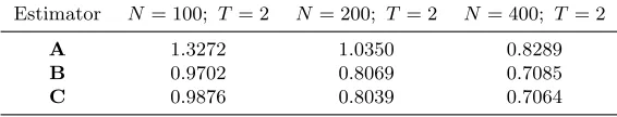
Table 1 reports the results of the experiment. We study the finite sample performance of our estimator (3.13) in comparison to a “naive” varying coefficient model with fixed effects that ignores endogenous selection (labelled “A”). The “naive” estimator is that of Sun et al. (2009), which is likely to produce inconsistent estimates of the unknown coefficient functionβ(·) due to its inability to account for the presence of sample selection effects. It is convenient to think of this estimator as a limiting case of our estimator (3.13) with the bandwidthh0 (for a single index in the selection
equation ∆w′ibγ) equal to infinity. In order to gauge the sensitivity of our estimator’s performance to a sampling error in the first-stage estimates, we also re-estimate our model using true values of
γ1 andγ2 (labelled “B”), i.e., with the first stage skipped. Our proposed two-stage estimator (3.13)
is labelled “C”.
[insert Table 1]
For each estimator in each simulation, we compute the root mean squared error (RMSE):
RM SE= P 1 N i=1
PT t=1φeidit
N
X
i=1
T
X
t=1 e
φidit
β(zit)−βb(zit)
2!1/2
, (5.2)
whereβb(·) is the estimate ofβ(·) from either of the three estimators A, B and C;φei ≡✶nPTt=1dit ≥2
o
“picks” cross-sections that are selected into the sample at least in two periods.
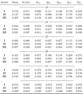
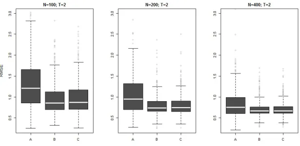
We summarize the results in Figure 1, where we plot distributions (across simulations) of the RMSE for each estimator and each sample size in the form of boxplots. We also report the averages of the RMSE computed over 500 simulations in Table 1. The results show that our estimator (C) is less biased than a “naive” estimator (A), which ignores endogenous selection. Comparing estimators B and C, we find that the results do not change dramatically if we use true or estimated values of
γ1 andγ2; the first-stage estimation seems to not distort the results obtained in the second stage.19
We also observe that the estimation (across all three estimators) becomes more stable as the sample size increases.
[insert Figure 1]
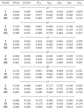
We next examine the finite sample performance of our estimator in the presence ofpolychotomous switching. Specifically, we considerR= 3. To make the experiment even more general, we setT = 3
17µ
i is generated so thatE[µi] = 0.
18Exactly in two periods in this experiment, becauseT= 2.
(the case of T >2). The DGP used is as follows [in line with (2.2)].
yr,it=
(
xr,itβr(zr,it) +µr,i+ur,it if dr,it= 1
− otherwise
d∗r,it=w1,itγr,1+w2,itγr,2+ξr,i+er,it
dr,it=✶{d∗r,it≥ max j=1,...,R;j6=r{d
∗
j,it}} , (5.3)
where the varying coefficients in the outcome equations are β1(z1,it) = sin(πz1,it), β2(z2,it) = 1 +
z2,it+(z2,it)2andβ3(z3,it) = 1+(z3,it)3 for regimes 1, 2 and 3, respectively. The constant coefficients in each of the three selection equations areγr,1 =γr,2= 1 forr= 1, 2, 3. The exogenous covariates
are generated as follows: (w1,it, w2,it) ∼ i.i.d. N(0,1), xr,it = w1,it and zr,it ∼ i.i.d. U(0,0.5π) for
r = 1, 2, 3. The fixed effects areξr,i =w1,i+w2,i+0.5ςr,iandµr,i=xr,i+zr,i+̺r,i−0.5−0.25π, where (ςr,i, ̺r,i) ∼i.i.d. U(0,1) for r = 1, 2, 3. The error terms in the selection equations er,it are i.i.d the type I extreme-value (Gumbel) distributed with location and scale parameters set to zero and one, respectively. The disturbances in the outcome equations are generated asur,it=−er,it+ζr,it, where ζr,it∼i.i.d. N(0,1) forr = 1, 2, 3. We consider sample sizesN ={150, 300, 600}, for each of which we simulate the design 500 times.
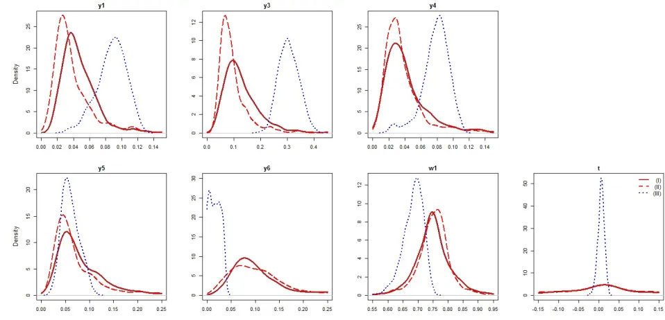
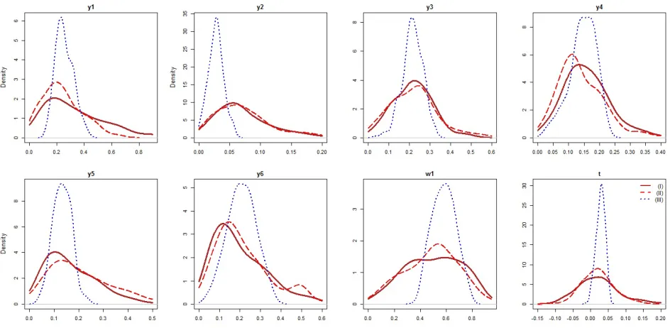
[insert Figure 2]
Since T = 3 in this design, in the second stage we estimate (3.13) for C(3,2) = 3 unique pairs of the time periods and then average βbr(·) for each zr,it, as discussed in Section 3.20 Also, note that the second stage is estimated for each regime separately. Figure 2 and Table 2 summarize the results from the three estimators, for each of the three regimes. The results are similar to those obtained in the case of binary sample selection. We find our estimator (C) to be less biased than a “naive” estimator (A) across all three regimes. The results do not seem to be sensitive to whether we use true or estimated values of the parameters in the selection equations (compare RMSE for estimators B and C). Importantly, the estimation becomes more stable as the sample size increases.
[insert Table 2]
6
Empirical Application: the Case of U.S. Credit Unions
In this section, we investigate the U.S. retail credit union production technologies in the period from 2002 to 2006. Using our proposed estimator (3.13), we are able to produce more robust estimates of credit union production technologies by controlling for (i) parameter heterogeneity in the cost function across credit unions of different sizes, (ii) endogenous selectivity as represented by differing service menus offered by credit unions and (iii) unobserved credit-union-specific heterogeneity. Be-fore we proceed, we note that the notation used in this section has no connection to that in previous sections, unless specified otherwise.
6.1 Framework and Data Description
Given that, due to their cooperative nature, credit unions are not profit-maximizers, researchers usually think of them as maximizing service provision to their members in terms of quantity, price
20In order to facilitate comparability of the results across estimators, we similarly estimate the “naive” estimator
and variety of services (Smith, 1984). We therefore follow a common practice in the credit union literature (Frame et al., 2003; Wheelock and Wilson, 2011, 2013) and adopt a “service provision approach.” According to this framework, given the type of their production technology,21 credit unions minimize non-interest, variable cost subject to the levels and types of services (outputs), the competitive prices of variable inputs and the levels of quasi-fixed netputs.
We consider four types of financial services that credit unions offer to their customers: real estate loans (y1), business and agricultural loans (y2), consumer loans (y3) and investments (y4). These are output quantities. We further follow Frame et al. (2003) and Wheelock and Wilson (2011, 2013) and include two quasi-fixed netputs to capture the price dimension of the service provision by credit unions: the average interest rate on saving deposits (ye5) and (the inverse of) the average interest rate on loans (ye6). The motivation here is to capture the cooperative nature of credit unions that, among other things, seek to offer the highest deposit rates and lowest loan rates possible to their members. Like Wheelock and Wilson (2011, 2013), one thus may prefer thinking of these price variables as quasi-fixed outputs. We therefore consider the inverse of the average interest rate on loans to enforce positive monotonicity (in outputs) of the cost function. Like Frame et al. (2003), we define two variable inputs: financial capital (x1) and labor (x2) with the vector of corresponding competitive prices w = (w1, w2). All of the above variables are taken as arguments of the dual variable, non-interest cost function of a credit union.
As pointed out in the Introduction, the data on credit unions contain a large number of ob-servations for which the reported values of some types of services are zeros, which indicates the presence of significant differences among credit unions in terms of the service menu they offer to members. Ignoring this observed heterogeneity in the provision of services amounts to making a strong and rather unrealistic assumption that all credit unions share the same technology that is invariant to the menu of services they provide. This assumption of homogeneous technology across credit unions is likely to result in the loss of information and the misspecification of the econometric model, which is further aggravated if the choice of the differing service menus by credit unions is endogenous. Malikov et al. (2013) document that the overwhelming majority of U.S. retail, or so-called natural-person, credit unions (more than 99%) offer one of the following three service menus to their members: (i) consumer loans and investments (y3, y4); (ii) real estate and consumer loans as well as investments (y1, y3, y4); and (iii) all types of services: real estate, business and consumer loans, and investments (y1, y2, y3, y4). We label these service menus (output mixes) as “1”, “2” and “3”, respectively, and refer to corresponding credit unions as “Type 1”, “Type 2” and “Type 3”. We hereafter use credit union and service menu types interchangeably when referring to credit unions and their production technologies.
The data come from year-end Call Reports available from the National Credit Union Adminis-tration (NCUA), a federal regulatory body that supervises all state and federally chartered credit unions in the U.S. In this study, we focus on the period prior to the 2008 financial crisis, in an attempt to minimize the influence of potential structural changes in the industry during the crisis and in its aftermath on the estimation results. In particular, we consider a five-year period from 2002 and 2006. We focus on retail credit unions only22and therefore exclude corporate credit unions (whose customers are the retail credit unions) from the sample to minimize noise in the data due to apparent non-homogeneity between these two types of unions.23
21That is, given the mix of financial services that credit unions choose to provide to their members.
22That is, we focus on retail credit unions of Types 1, 2 or 3. Credit unions that offer other service menus (less than
a percent of observations) likely contain either outliers or reporting errors.
23We also discard observations with negative values of outputs and total cost. In addition, we exclude observations
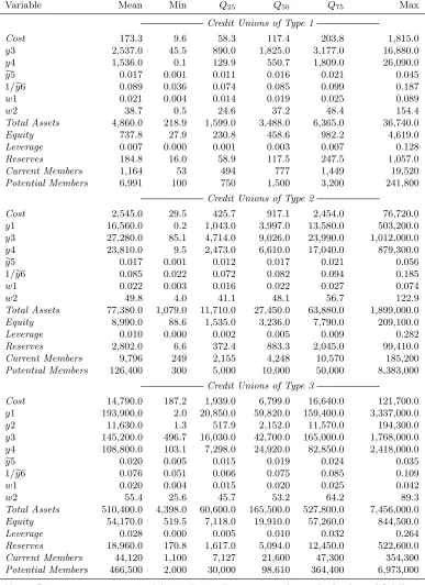
Recall that, in order to make our proposed estimator feasible, one needs (i) cross-sections to switch regimes (to estimate the selection equations in the first stage) and (ii) a given regime to be selected by a cross-sectional unit at least in two time periods (to estimate the outcome equation in the second stage). We therefore confine our analysis to credit unions that meet the above two requirements. Also, to avoid a potential impact of entries and exits, we examine only continuously operating credit unions. Lastly, given significant computational intensity of our proposed estimator (particularly, a cross-validation procedure in the second stage), we select a pseudo-random repre-sentative subsample of credit unions satisfying all above criteria, which renders a balanced panel of 500 units continuously observed over 5 years. The procedure does not significantly affect the distribution of key variables and the composure over credit union types.24
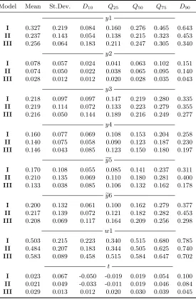
Table 3 reports summary statistics of the variables used in our analysis. We deflate all nominal stock variables to 2011 U.S. dollars using the GDP Implicit Price Deflator. A comparison of sample mean and median estimates of variables shows clear differences between the credit union types. As expected, the size of the credit unions (proxied either by total assets or the number of members) increases as one moves from Type 1 to Type 3. The dramatic differences between the three types favor our view that the assumption of homogeneous credit union technology across service menu types is likely to result in the loss of information and the misspecification of the econometric model. Moreover, credit unions technology is also unlikely to be homogenous within a given service menu type, which, if overlooked, can distort results as well.
[insert Table 3]
To put the problem of modeling credit union technologies into perspective of the estimator that we consider in this paper, there are three distinct types of retail credit unions, as defined by their differing service menus. These types are what we have referred to in the previous sections as polychotomous “regimes”. Since there are no legal restrictions on which of the four financial services (outputs) a credit union may offer to its members, it is natural to view these credit union types as an outcome of endogenous decision-making. The data seem to suggest that the variables capturing a credit union’s size, financial strength and potential for growth may be particularly relevant to a choice of the service menu. A careful examination of the credit union literature suggests considering the following variables: the number of current and potential members, equity capital,25reserves and
the leverage ratio, defined as the ratio of total debt to total assets (Bauer, 2008; Bauer et al., 2009; Goddard et al., 2002, 2008).26 These are the variables entering the selection equations. For their summary statistics, see Table 3.
Further, it has been argued in the literature that the size of a credit union (commonly measured by its total assets) matters considerably in shaping its cost structure and that any parametric spec-ification of the cost function that overlooks this relationship is thus likely to suffer from parameter instability (Wheelock and Wilson, 2011). We concur with this sentiment and agree that it may be inappropriate to assume that the cost structure of a small credit union is the same as that of a large credit union. To accommodate this technological heterogeneity among credit unions of different sizes, we allow parameters of the credit-union-type-specific cost function to also be varying with (the log of) credit union’s total assets. Such a specification yields credit-union-specific estimates of
lie outside the unit interval. These excluded observations are likely to be the result of erroneous data reporting. All variables are constructed following the instructions in the appendix of Malikov et al. (2013).
24We have tried numerous pseudo-random subsample, all of which yield qualitatively unchanged results. The
compo-sition of the sample by credit union types is 28%, 60% and 12% for Types 1, 2 and 3, respectively.
25We note that, since credit unions are mutual organizations, they cannot raise “equity” via public offering per se.
The equity is instead raised by retaining earnings.
the cost function parameters.
6.2 Estimation and Empirical Results
We consider a VC model of heterogeneous credit union production technologies with polychotomous endogenous switching and fixed effects in both the selection and outcome equations. In this paper, we assume that the credit-union-type-specific dual cost function takes a semiparametric analogue of the translog specification, under which parameters are unknown smooth functions of the size. We cast the model in the form of (2.2), i.e.,
lnCitr =µr(zit) +η1r(zit) t+ 1 2η
r
11(zit) t2+ Mr
X
m=1
βmr(zit) lnym,itr + 1 2 Mr X m=1 Mr X h=1
βmhr (zit) lnym,itr lnyh,itr + Mr
X
m=1
ρrm1(zit) lnyrm,itt+
K
X
k=1
ωkr(zit) lnyek,it+ 1 2 K X k=1 K X g=1
ωrkg(zit) lneyk,itlnyeg,it+ K
X
k=1
ρrk2(zit) lneyk,it t+
J
X
j=1
δjr(zit) lnwj,it+ 1 2 J X j=1 J X s=1
δjsr (zit) lnwj,itlnws,it+ J
X
j=1
ρrj3(zit) lnwj,it t+
Mr X m=1 J X j=1
θrmj(zit) lnyrm,itlnwj,it+ K X k=1 J X j=1
ϑrkj(zit) lnyek,itlnwj,it+
Mr X m=1 K X k=1
̺rmk(zit) lnyrm,itlnyek,it+µri +urit (if drit= 1) (6.1a)
dr∗it = H
X
h=1
γhrlnqh,it+ξir+erit , (i= 1, . . . , N; t= 1, . . . , T; R = 1, . . . , R) (6.1b)
where, for each credit union typer= 1, . . . , R(R= 3),Citr is the variable, non-interest cost; yrm,it∈
yritis the output specific to a given type of credit unions, i.e.,y1it≡(y3it, y4it),y2it≡(y1it, y3it, y4it),
y3it ≡ (y1it, y2it, y3it, y4it) with the corresponding values of Mr = {2, 3, 4}. The variable input priceswj,it∈(w1, w2), quasi-fixed netputsyek,it ∈(ye5,ye6) and the log of total assetszitare invariant to credit union type and thus do not have superscript r (also, J =K = 2). To capture temporal changes in the cost frontiers, we also include the time trend t in (6.1a). The rth cost function is observed if a credit union selects the rth type of the service mix, as captured by the binary indicatordrit. The selection is governed by (6.1b) that assumes that the propensity to select therth service mix type is a function of qit that includes the number of current and potential members, equity capital, reserves and the leverage ratio (H = 5). We control for unobserved unit-specific heterogeneity among credit unions by including fixed effects µri and ξir in the cost and selection equations, respectively.
We estimate the model in two stages as outlined in Section 3. In the first stage, we transform (6.1b) into its binary selection analogue as described in Section 2.2, which is then estimated via Chamberlain’s (1980) conditional multinomial logit. We use the obtained estimates of parameters
b