On the Stratonovich – Kalman Bucy filtering algorithm application for accurate characterization of financial time series with use of state space model by central banks

Munich Personal RePEc Archive

On the Stratonovich – Kalman - Bucy

filtering algorithm application for

accurate characterization of financial

time series with use of state-space model

by central banks

Ledenyov, Dimitri O. and Ledenyov, Viktor O.

James Cook University Townsville Australia

27 September 2013

1 On the Stratonovich – Kalman - Bucy filtering algorithm application for

accurate characterization of financial time series with use of state-space

model by central banks

Dimitri O. Ledenyov and Viktor O. Ledenyov

Abstract – The central banks introduce and implement the monetary and financial stabilities policies, going from the accurate estimations of national macro-financial indicators such as the Gross Domestic Product (GDP). Analyzing the dependence of the GDP on the time, the central banks accurately estimate the missing observations in the financial time series with the application of different interpolation models, based on the various filtering algorithms. The Stratonovich – Kalman – Bucy filtering algorithm in the state space interpolation model is used with the purpose to interpolate the real GDP by the US Federal Reserve and other central banks. We overviewed the Stratonovich – Kalman – Bucy filtering algorithm theory and its numerous applications. We describe the technique of the accurate characterization of the economic and financial time series with application of state space methods with theStratonovich – Kalman - Bucy filtering algorithm, focusing on the estimation of Gross Domestic Product by the Swiss National Bank. Applying the integrative thinking principles, we developed the software program and performed the computer modeling, using the Stratonovich – Kalman – Bucy filtering algorithm for the accurate characterization of the Australian GDP, German GDP and the USA GDP in the frames of the state-space model in Matlab. We also used the Hodrick-Prescott filter to estimate the corresponding output gaps in Australia, Germany and the USA. We found that the Australia, Germany on one side and the USA on other side have the different business cycles. We believe that the central banks can use our special software program with the aim to greatly improve the national macroeconomic indicators forecast by making the accurate characterization of the financial time-series with the application of the state-space models, based on the Stratonovich – Kalman – Bucy filtering algorithm.

JEL: C15, C32, C51, C52, E5, E31, E32.

PACS numbers: 89.65.Gh, 89.65.-s, 89.75.Fb .

Keywords: Wiener filtering theory, Stratonovich optimal non-linear filtering theory,

2 Introduction

The economic and financial principles by the Austrian school of economic thinking in Menger (1871), von Böhm-Bawerk (1884, 1889, 1921), von Mises (1912, 1949), Hayek (1931, 1935, 1948, 1980, 2008), Hazlitt (1946), Rothbard (1962, 2004) had a considerable scientific influence on the modern Monetarism theories by the American scientists of the Austrian origin at the Chicago school of economic thinking in the XX – XXI centuries. In our time, the Chicago school of economic thinking has a reputation of a world renowned expert in the finances, influencing the US policymakers, governmental officials, congressmen, senators, who work on the US Federal Reserve System governance policies introduction and execution. The central bank of the United States, the US Federal Reserve System, was founded in the Federal Reserve Act, passed by the US Congress in 1913 in Willis (1923), Meltzer (2003, 2009a, b), Bernanke (2013). The main purpose of the US Federal Reserve System was: “provide a means by which periodic panics which shake the American Republic and do it enormous injury shall be stopped” in Owen (1919), Bernanke (2013). Analyzing the historical developments, Dr. Ben Shalom Bernanke, Chairman of the US Federal Reserve System distinguishes the following historical periods in the US Federal Reserve System operation in Bernanke (2013): 1) The Great Experiment of the US Federal Reserve System founding in 1913; 2) The Great Depression in 1922–1933; 3) The Stable Inflation in 1950s – 1960s, Great Inflation in mid 1960s – end 1970s, and Disinflation in 1979–1984; 4) The Great Moderation in 1984–2007; 5) The Great Recession in 2008–until now. In Fig. 1, the first Federal Reserve System Board in 1914 is shown in Fox, Alvarez, Braunstein, Emerson, Johnson, Johnson, Malphrus, Reinhart, Roseman, Spillenkothen, Stockton (2005).

3

As the principal monetary authority of a nation, the US Federal Reserve System (central bank) performs the key functions towards the introduction and implementation of:

1. Monetary stability policy, aiming to stabilize the prices and increase the confidence in the currency by setting and reaching the inflation target through the realization of transparent effective programs on the interest rates and asset purchases in the money markets, and

2. Financial stability policy, aiming to detect and reduce the systemic risks to the national financial system by identifying and monitoring the possible systemic threats to the financial stability and by taking an action to reduce those threats by improving the financial infrastructure, by setting the banking capital requirements, by acting as the lender of last resort.

Presently, the US Federal Reserve System’s main purpose is to provide the nation with a safer, more flexible, and more stable monetary and financial system in Fox, Alvarez, Braunstein, Emerson, Johnson, Johnson, Malphrus, Reinhart, Roseman, Spillenkothen, Stockton (2005).

The Federal Reserve System’s main duties are in Fox, Alvarez, Braunstein, Emerson, Johnson, Johnson, Malphrus, Reinhart, Roseman, Spillenkothen, Stockton (2005):

1. Conducting the nation’s monetary policy by influencing the monetary and credit conditions in the economy in pursuit of maximum employment, stable prices, and moderate long-term interest rates.

2. Supervising and regulating the banking institutions to ensure the safety and soundness of the nation’s banking and financial system and to protect the credit rights of consumers.

3. Maintaining the stability of the financial system and containing systemic risk that may arise in financial markets.

4. Providing the financial services to depository institutions, the US Government, and foreign official institutions, including playing a major role in operating the nation’s payments system.

4

operations, imposing reserve requirements, permitting depository institutions to hold contractual clearing balances, and extending credit through its discount window facility, the Federal Reserve exercises considerable control over the demand for and supply of Federal Reserve balances and the federal funds rate. Through its control of the federal funds rate, the Federal Reserve is able to foster financial and monetary conditions consistent with its monetary policy objectives.”

In Fig. 2, the US Federal Reserve System is depicted in Fox, Alvarez, Braunstein, Emerson, Johnson, Johnson, Malphrus, Reinhart, Roseman, Spillenkothen, Stockton (2005).

5

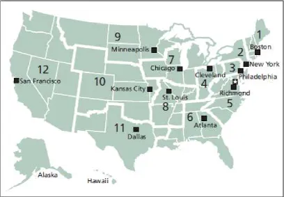
In Tab. 1, the US Federal Reserve district banks and branches are shown in Fox, Alvarez, Braunstein, Emerson, Johnson, Johnson, Malphrus, Reinhart, Roseman, Spillenkothen, Stockton (2005).

6

In Fig. 3, the market for balances at the US Federal Reserve is shown in Fox, Alvarez, Braunstein, Emerson, Johnson, Johnson, Malphrus, Reinhart, Roseman, Spillenkothen, Stockton (2005).

Fig. 3. The market for balances at the US Federal Reserve (after Fox, Alvarez, Braunstein, Emerson, Johnson, Johnson, Malphrus, Reinhart, Roseman, Spillenkothen, Stockton (2005)).

The central bank’s monetary policy is usually guided by the basic principles and needs to be flexible enough to respond to the financial fluctuations in the capital markets in Ferguson (2003). In the researched case of the Swiss National Bank (SNB), the SNB’s “best-practice” monetary policy framework is based on the following important principles in Baltensperger, Hildebrand, Jordan (2007):

1. Priority given to long-term price stability as a firm nominal anchor, with an explicit quantitative definition of what is meant by price stability;

2. A medium-term orientation in the pursuit of this objective, giving scope for short-run flexibility to dampen real economic fluctuations;

3. A forward-looking approach in the pursuit of its objectives, through the use of an inflation forecast as its main indicator;

4. Flexible implementation of monetary policy, through the announcement of a target range for the three-month CHF Libor as an operational target;

7

Let us explain that the central banks introduce the changes into the monetary stability policy and the financial stability policy, going from the estimated economic and financial indicators such as the Gross Domestic Product (GDP) in Taylor (1999). Aiming to complete the accurate characterizations of the different economic and financial indicators, the central banks estimate the missing observations in the various economic time series with the application of the different interpolation models, including the state-space model, in Bernanke, Gertler, Watson (1997), Cuche, Hess (2000). The Stratonovich – Kalman – Bucy filtering algorithm in Stratonovich (1959a, b, 1960a, b), Kalman, Koepcke (1958, 1959), Kalman, Bertram (1958, 1959), Kalman (1960a, b, 1963), Kalman, Bucy (1961) represents one of the possible interpolation models, which has been effectively used to interpolate the real Gross Domestic Product (GDP) by the Federal Reserve in the USA, Swiss National Bank in Switzerland and by some other central banks in various countries in Bernanke, Gertler, Watson (1997), Cuche, Hess (2000), Proietti, Luati (2012a).

The other macroeconomic applications of the state-space interpolation models may also include in Proietti, Luati (2012a):

• The extraction of signals such as trends and cycles in macroeconomic time series: see Watson (1986), Clark (1987), Harvey and Jaeger (1993), Hodrick and Prescott (1997), Morley, Nelson and Zivot (2003), Proietti (2006), Luati and Proietti (2011).

• The dynamic factor models, for the extraction of a single index of coincident indicators, see Stock and Watson (1989), Frale et al. (2011), and for large dimensional systems Jungbacker, Koopman and van der Wel (2011).

• The stochastic volatility models: see Shephard (2005) and Stock and Watson (2007) for applications to US inflation.

• The time varying auto-regressions with stochastic volatility: see Primiceri (2005), Cogley, Primiceri and Sargent (2010).

• The structural change in macroeconomics: see Kim and Nelson (1999).

• The class of dynamic stochastic general equilibrium (DSGE) models: see Sargent (1989), Villaverde and Rubio-Ramirez (2005), Smets and Wouters (2003), Fernandez-Villaverde (2010).

8 Stratonovich – Kalman – Bucy filtering algorithm and its applications

The Stratonovich – Kalman – Bucy filtering algorithm was invented in the science of radio-physics, hence let us make a brief overview of the analogue and digital signals processing techniques with the purpose to understand an essence of the Stratonovich – Kalman – Bucy filtering algorithm in Stratonovich (1959a, b, 1960a, b), Kalman, Koepcke (1958, 1959), Kalman, Bertram (1958, 1959), Kalman (1960a, b, 1963), Kalman, Bucy (1961).

Discussing the analogue signal processing, it is worth to say that, in the theory of electrodynamics and the theory of radio-physics, it is a well known fact that the analogue signal with the encoded information can be transmitted by the signal carrier over the wireless, wireline or optical channels in Wanhammar (1999), Ledenyov D O, Ledenyov V O (2012e). This analogue signal can be accurately characterized by its changing amplitude, frequency, phase and power over the certain time period in Ledenyov D O, Ledenyov V O (2012e). The encoding of the information into the analogue signal can be done with the help of various modulation processes by changing the analogue signal’s parameters such as the amplitude (amplitude modulation), frequency (frequency modulation), phase (phase modulation) and power (pulse code modulation) over the time in Ledenyov D O, Ledenyov V O (2012e). The analogue signal can be continuously transmitted over the transmission channel for some time period (the continuous wave (CW) signal) or it can be discretely transmitted over the transmission channel for some time(the discrete signal). In the last case, the analogue signal can be represented as a sequence of the

discrete magnitudes of physical parameters of the analogue signal in Ledenyov D O, Ledenyov V O (2012e). The analogue signals filtering with the frequency

selective signal filters is needed in the cases, when it is necessary to transmit or receive the selected analogue signal over the certain frequency in the frequency domain only in Ledenyov D O, Ledenyov V O (2012e). The analogue signals filtering is well described in the book: “Nonlinearities in microwave superconductivity” in Ledenyov D O, Ledenyov V O (2012e): “The High Temperature Superconducting (HTS) microwave electromagnetic signal filter is one of the essential microwave components in modern wireless communication systems in which the complete and independent measurement of the entire signal space to identify and decode the information in the spectral transmission sequences over the wireless channel is made. The main functions of microwave filter are to select the information signal carrier in the frequency domain and amplify its amplitude by the resonance.”

9

the help of the Analogue to Digital (A/D) converter to obtain the digital signal; or the digital signal can be de-sampled over the time with the help of the Digital to Analogue (D/A) converter to obtain the analogue signal in Wanhammar (1999). The analogue signal processing can be performed, using the analogue signal processing algorithms such as the Fourier transform, Laplace transform, etc. in Wanhammar (1999). The digital signal processing can be performed, using the digital signal processing algorithms such as the Discrete Fourier transform (DFT), Fast Fourier transform (FFT), Cooley-Turkey Fast Fourier transform (CT FFT), Sande-Tukey Fast Fourier transform (ST FFT), Inverse Fast Fourier transform (Inverse FFT), Discrete Cosine transform (DCT), Wavelet transform, z-transform, etc. in Wanhammar (1999). As explained in Wanhammar (1999): “The main purpose of a signal processing system is generally to reduce or retain the information in a signal.” The digital signal processing is usually done for the Linear Shift Invariant (LSI) systems, which are linear and time-invariant in Wanhammar (1999). The frequency response of the Linear Shift Invariant (LSI) system can be characterized by the frequency function, magnitude function, attenuation function, phase function, group delay function, and transfer function in Wanhammar (1999). The digital filters can also be classified in the Finite-length Impulse Response (FIR) filters and Infinite-length Impulse Response (IIR) filters, depending on their response functions characteristics in Wanhammar (1999).

Going to the discussion on the Stratonovich – Kalman – Bucy filtering algorithm, it is interesting to highlight the fact that, since the beginning of the XX century, the nonlinearities

and nonlinear physical systems represented the subjects of strong research interest in the natural sciences, including the radio-physics (the analogue signal processing) in Mandel’shtam (1948-1955), Andronov (1956), Rytov (1957); the nuclear physics in Fermi, Pasta, Ulam (1955), Femi (1971-1972). The nonlinearities in the microwave superconductivity were comprehensively researched in Ledenyov D O, Ledenyov V O (2012e).

Analyzing the time series, Ruslan L. Stratonovich created the optimal non-linear filtering theory in 1959 in Stratonovich (1959a, b, 1960a, b). During next few years, the optimal non-linear filtering theory has been extensively complemented by the various research findings; and its foundational principles have been used to develop the Stratonovich – Kalman – Bucy filtering algorithm in 1959-1963 in Stratonovich (1959a, b, 1960a, b), Kalman, Koepcke (1958, 1959), Kalman, Bertram (1958, 1959), Kalman (1960a, b, 1963), Kalman, Bucy (1961).

10

those based on a single measurement alone. More formally, the Kalman filter operates recursively on streams of noisy input data to produce a statistically optimal estimate of the underlying system state. The filter is named for Rudolf (Rudy) E. Kálmán, one of the primary developers of its theory.”

The Stratonovich – Kalman – Bucy filtering algorithm is also described in Wikipedia (2013): “The algorithm works in a two-step process. In the prediction step, the Kalman filter produces estimates of the current state variables, along with their uncertainties. Once the outcome of the next measurement (necessarily corrupted with some amount of error, including random noise) is observed, these estimates are updated using a weighted average, with more weight being given to estimates with higher certainty. Because of the algorithm's recursive nature, it can run in real time using only the present input measurements and the previously calculated state; no additional past information is required.”

Athans (1974) write: "The Kalman filter represents one of the major contributions in modern control theory. Since its original development (references [I] and [2]), it has been rederived from several points of view bringing into focus its properties from both a probabilistic and optimization viewpoint (references [3] to [9]). Its importance in stochastic control can be appreciated in view of the numerous applications (references [5], [6], [9] to [16])."

Kleeman (1995) explains: “A Kalman filter is an optimal estimator – i.e. it infers parameters of interest from indirect, inaccurate and uncertain observations. The process of finding the “best estimate” from noisy data amounts to “filtering out” the noise. If all noise is Gaussian, the Kalman filter minimizes the mean square error of the estimated parameters. However a Kalman filter also doesn’t just clean up the data measurements, but also projects these measurements onto the state estimate.”

Welch, Bishop (2001) notes: “The Kalman filter is essentially a set of mathematical equations that implement a predictor-corrector type estimator that is optimal in the sense that it minimizes the estimated error covariance—when some presumed conditions are met.”

11

Minimum Mean Squared Error estimator if the observed variable and the noise are jointly Gaussian.”

Proietti, Luati (2012a) come up with the explanation: “The Kalman filter (Kalman, 1960; Kalman and Bucy, 1961) is a fundamental algorithm for the statistical treatment of a state space model. Under the Gaussian assumption, it produces the minimum mean square estimator of the state vector along with its mean square error matrix, conditional on past information; this is used to build the one-step-ahead predictor of yt and its mean square error matrix. Due to the

independence of the one-step-ahead prediction errors, the likelihood can be evaluated via the prediction error decomposition.”

It is possible to think about the Stratonovich – Kalman – Bucy filter as a device, which can estimate the state of a dynamic system from a series of incomplete and noisy measurements. It can be used to predict a current state by using the previous one, or estimate an updated state by using the previous state and current measurement. The predicted and estimated measurements are calculated from their corresponding states as discussed in Matlab (R2012).

The Stratonovich – Kalman – Bucy filtering algorithm is extensively used in the following types of signal processing filters in Wikipedia (2013): the alpha beta filter, ensemble Kalman filter, extended Kalman filter, iterated extended Kalman filter, fast Kalman filter, invariant extended Kalman filter, kernel adaptive Kalman filter, non-linear Kalman filter, Schmidt–Kalman filter, hybrid Kalman filter, and Wiener filter as explainedin Jazwinski (1970), Bozic (1979),Bar-Shalom, Maybeck (1990), Xiao-Rong Li (1993).

There is a big number of practical technical applications of the Stratonovich – Kalman – Bucy filtering algorithm, for example: the Fast Stratonovich – Kalman – Bucy adaptive filter is implemented in the equalizers with the short training times in Wanhammar (1999). In the general case, the equalization of wireless channel is achieved by the application of the digital filters such as the Recursive Least Square (RLS) lattice filters with the aim to compensate for the various distortions in the wireless channel and to eliminate the inter-symbol interference in the chips sequence during the spread spectrum communication over the wireless channel, because of the Ritz RF signal fading model or the Raleigh RF signal fading model, for instance, in the cases of both the Wideband Code Division Multiple Access (WCDMA) communication or the Direct Sequence Spread Spectrum (DSSS) communication over the constantly fading wireless channel in Wanhammar (1999), Ledenyov D O, Ledenyov V O (2012e).

12

spread spectrum signals communications, tracking and vertex fitting of charged particles in particle detectors systems, tracking of objects in computer vision systems, GDP interpolation in macroeconomics, Volterra series interpolation in economics, inertial guidance systems in on board navigation systems, radar tracking systems, GPS satellite navigation systems, systems for sensor-less control of AC motor variable-frequency drives.

Stratonovich – Kalman – Bucy filtering algorithm theory

Let us begin with the comprehensive discussion on the Stratonovich – Kalman – Bucy filtering algorithm theory by bringing some interesting facts on the history of science to our close attention. Wiener (1949) completed a research on the extrapolation, interpolation and smoothing of stationary time series. Stratonovich (1959a, b) made a research on the selection of the useful signals from the noise in the nonlinear systems, attempting to create the theory of optimal non-linear filtering of random functions. Stratonovich (1960a, b) applied the Markov processes theory to the theory of optimal non-linear filtering. Kalman, Koepcke (1958a, 1959b), Kalman, Bertram (1958b, 1959a), Kalman (1960a) conducted the innovative researches on the theory of linear sampling control systems. At later date, Kalman (1960b) focused on the linear filtering and prediction research problems, formulating and solving the Wiener problem from the “state” point of view. Kalman (1963) accented his research attention on the development of new methods in the Wiener filtering theory. Let us emphasis that Kalman (1960b) considered some theoretical aspects of both the general linear continuous-dynamic system and the general linear discrete-dynamic system.

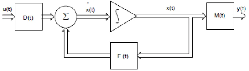
The block diagram of the general linear continuous-dynamic system is shown in Fig. 4 and the block diagram of the general linear discrete-dynamic system is depicted in Fig. 5 in Kalman (1960b).

13

Fig. 5. Matrix block diagram of the general linear discrete-dynamic system (after Kalman (1960b)).

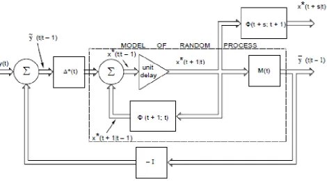
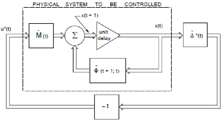
The block diagram of optimal filter is shown in Fig. 6 and the block diagram of optimal controller is represented in Fig. 7 in Kalman (1960b).

14

Fig. 7. Matrix block diagram of optimal controller(after Kalman (1960b)).

Let us learn more on the theory of the Stratonovich – Kalman – Bucy filtering in Wikipedia (2013): “The Kalman filters are based on linear dynamic systems discretized in the time domain. They are modeled on a Markov chain built on linear operators perturbed by Gaussian noise. The state of the system is represented as a vector of real numbers. At each discrete time increment, a linear operator is applied to the state to generate the new state, with some noise mixed in, and optionally some information from the controls on the system if they are known. Then, another linear operator mixed with more noise generates the observed outputs from the true ("hidden") state. The Kalman filter may be regarded as analogous to the hidden Markov model, with the key difference that the hidden state variables take values in a continuous space (as opposed to a discrete state space as in the hidden Markov model). Additionally, the hidden Markov model can represent an arbitrary distribution for the next value of the state variables, in contrast to the Gaussian noise model that is used for the Kalman filter. There is a strong duality between the equations of the Kalman Filter and those of the hidden Markov model”.

The Kalman filter model assumes the true state at time k is evolved from the state at (k−1) according to in Wikipedia (2013)

where Fk is the state transition model, which is applied to the previous state xk−1;

Bk is the control-input model which is applied to the control vector uk;

1

k k k k k k

15 wk is the process noise which is assumed to be drawn from a zero mean multivariate normal

distribution with covariance Qk.

At time k an observation (or measurement) zk of the true state xk is made according to in

Wikipedia (2013)

where Hk is the observation model, which maps the true state space into the observed space and

vk is the observation noise, which is assumed to be zero mean Gaussian white noise with

covariance Rk.

The initial state, and the noise vectors at each step {x0, w1, ..., wk, v1 ... vk} are all

assumed to be mutually independent.

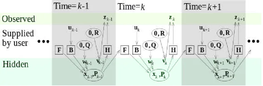
In Fig. 8, the model, underlying the Kalman filter is shown in Wikipedia (2013).

Fig. 8. Model underlying the Kalman filter. Squares represent matrices. Ellipses represent multivariate normal distributions (with the mean and covariance matrix enclosed). Unenclosed values are vectors. In the simple case, the various matrices are constant with time, and thus the subscripts are dropped, but the Kalman filter allows any of them to change each time step (after

Wikipedia (2013)).

(

0,

)

k k

w



N

Q

k k k k

z

=

H x

+

v

(

0,

)

k k

16

“The Kalman filter is a recursive estimator. This means that only the estimated state from the previous time step and the current measurement are needed to compute the estimate for the current state. In contrast to batch estimation techniques, no history of observations and/or estimates is required. In what follows, the notation represents the estimate of x at time n given observations up to, and including at time m,” as explained in Wikipedia (2013).

The state of the Kalman filter is represented by the two variables in Wikipedia (2013): 1. , the a posteriori state estimate at time k given observations up to and including at time k; 2. , the a posteriori error covariance matrix (a measure of the estimated accuracy of the state estimate).

“The Kalman filter can be written as a single equation, however it is most often conceptualized as two distinct phases: "Predict" and "Update". The predict phase uses the state estimate from the previous timestep to produce an estimate of the state at the current timestep. This predicted state estimate is also known as the a priori state estimate because, although it is an estimate of the state at the current timestep, it does not include observation information from the current timestep. In the update phase, the current a priori prediction is combined with current observation information to refine the state estimate. This improved estimate is termed the a posteriori state estimate.

Typically, the two phases alternate, with the prediction advancing the state until the next scheduled observation, and the update incorporating the observation. However, this is not necessary; if an observation is unavailable for some reason, the update may be skipped and multiple prediction steps performed. Likewise, if multiple independent observations are available at the same time, multiple update steps may be performed (typically with different observation matrices Hk),” as explained in Wikipedia (2013).

Predict phase:

Predicted (a priori) state estimate:

Predicted (a priori) estimate covariance:

Update phase:

Innovation or measurement residual:

Innovation (or residual) covariance:

ˆ

x

ˆ

x

k k

P

1 1

1 1 1

ˆ

ˆ

x

=

F x

+

B

u

1 1 1

T

k k k

k k k k

P

=

F P

F

+

Q

1

ˆ

k k k k k

y



=

z

−

H x

1

T

k k k k k k

17

Optimal Kalman gain:

Updated (a posteriori) state estimate:

Updated (a posteriori) estimate covariance:

Invariants:

“If the model is accurate, and the values for and accurately reflect the distribution of the initial state values, then the following invariants are preserved: (all the estimates have a mean error of zero),” see in Wikipedia (2013)

where is the expected value of ξ, and the covariance matrices accurately reflect the covariance of estimates in Wikipedia (2013)

Let us express a general opinion in Wikipedia (2013): “Practical implementation of the Kalman filter is often difficult due to the inability in getting a good estimate of the noise covariance matrices Qk and Rk. Extensive research has been done in this field to estimate these

covariances from data. One of the more promising approaches to do this is the Autocovariance Least-Squares (ALS) technique that uses autocovariances of routine operating data to estimate the covariances in Rajamani (2007), Rajamani, Rawlings (2009).”

Let us provide an additional comment in Wikipedia (2013): “It is known from the theory that the Kalman filter is optimal in case that

a) the model perfectly matches the real system,

1 1

T

k k k k k

K

=

P

H S

1 1

ˆ

ˆ

x

=

x

+

K y



(

)

k k k k

P

= −

I

K H

P

1

ˆ

ˆ

0

k k k k k k

E x



_

−

x

_



=

E x



_

−

x



_

=

[ ]

0

E y



=

[ ]

E

ξ

(

ˆ

)

cov

k k k k

P

=

x

−

x

(

)

1

cov

ˆ

k k k k

P

=

x

−

x

( )

cov

k k

S

=

y



0 0

ˆ

18

b) the entering noise is white, and

c) the covariances of the noise are exactly known.

Several methods for the noise covariance estimation have been proposed during past decades. One, ALS, was mentioned in the previous paragraph. After the covariances are identified, it is useful to evaluate the performance of the filter, i.e. whether it is possible to improve the state estimation quality. It is well known that, if the Kalman filter works optimally, the innovation sequence (the output prediction error) is a white noise. The whiteness property reflects the state estimation quality. For evaluation of the filter performance it is necessary to inspect the whiteness property of the innovations. Several different methods can be used for this purpose. Three optimality tests with numerical examples are described in Matisko, Havlena (2012).”

We would like to explain that there are many types of algorithms for the recursive estimation, including the Stratonovich – Kalman – Bucy filteringalgorithm, the forgetting factor algorithm, the unnormalized and normalized gradient algorithm, which have been used to solve the different mathematical tasks in the system identification problem in Ljung (1999). The following set of equations summarizes the Stratonovich – Kalman – Bucy filtering algorithm in Matlab (R2012):

This formulation assumes the linear-regression form of the model in Matlab (R2012):

The Stratonovich – Kalman – Bucyfilter is used to obtain Q(t).

This formulation also assumes that the true parameters are described by a random walk in Matlab (R2012):

( )

(

)

( ) ( )

(

( )

)

( )

( ) (

)

( )

( ) ( )

( )

(

)

( ) (

) ( )

( )

(

)

(

) ( ) ( ) (

)

( ) (

) ( )

ˆ

ˆ

₁

_ˆ

ˆ

ˆ

1

1

1

1

1

1

1

θ

= θ − +

−

= Ψ

θ −

=

Ψ

−

=

+ Ψ

− Ψ

− Ψ

Ψ

−

=

− +

−

+ Ψ

− Ψ

T

T

T

T

t

t

K t

y t

y t

y t

t

t

K t

Q t

t

P t

Q t

R

t

P t

t

P t

t

t

P t

P t

P t

R

R

t

P t

t

( )

= Ψ

( ) ( ) ( )

θ

+

T

y t

t

t

e t

( )

19

where w(t) is the Gaussian white noise with the following covariance matrix, or drift matrix R1 in

Matlab (R2012):

R2 is the variance of the innovations e(t) in the following equation in Matlab (R2012):

The Stratonovich – Kalman – Bucy filtering algorithm is entirely specified by the sequence of data y(t), the gradient , R1, R2, and the initial conditions (initial

guess of the parameters) and (covariance matrix that indicates parameters errors in Matlab (R2012).

Summarizing the above research statements, we would like to say that the Stratonovich – Kalman – Bucy filtering is used to predict or estimate the state in the dynamic system. The Wiener filtering, Stratonovich – Kalman – Bucy filtering and related scientific problems have been extensively researched in the numerous scientific articles in Wiener (1949), Bartlett (1954), Tukey (1957), Stratonovich (1959a, b, 1960a, b), Kalman, Koepcke (1958, 1959), Kalman, Bertram (1958, 1959), Kalman (1960a, b, 1963), Kalman, Bucy (1961), Friedman (1962), Bryson, Ho (1969), Bucy, Joseph (1970), Jazwinski (1970), Sorenson (1970), Chow, Lin (1971, 1976), Maybeck (1972, 1974, 1990), Willner (1973), Leondes, Pearson (1973), Akaike (1974), Dempster, Laird, Rubin (1977), Griffiths (1977), Schwarz (1978), Falconer, Ljung (1978), Anderson, Moore (1979), Bozic (1979), Priestley (1981), Lewis (1986), Proakis, Manolakis (1988), Caines (1988), de Jong (1988, 1989, 1991), de Jong, Chu-Chun-Lin (1994), Bar-Shalom, Maybeck (1990), Franklin, Powell, Workman (1990), Brockwell, Davis (1991), Jang (1991), Brown, Hwang (1992, 1997), Xiao-Rong Li (1993), Gordon, Salmond, Smith (1993), Farhmeir, Tutz (1994), Grimble (1994), Lee, Ricker (1994), Ricker, Lee (1995), Fuller (1996), Hayes (1996), Haykin (1996), Golub, van Loan (1996), Julier, Uhlmann (1997), Ljung (1999), Wanhammar (1999), Welch, Bishop (2001), Litvin, Konrad, Karl (2003), de Jong, Penzer (2004), van Willigenburg, De Koning (2004), Voss, Timmer, Kurths (2004), Capp´e, Moulines, Ryd´en (2005), Misra, Enge (2006), Rajamani (2007), Andreasen (2008), Rajamani, Rawlings (2009), Xia Y, Tong H (2011), Matisko, Havlena (2012), Proietti, Luati (2012a, b), Durbin, Koopman (2012).

( )

(

)

( )

0 0

1

θ

t

= θ

t

− +

w t

( )

Ψ

t

( ) ( )

=

T

Ew t w t

R

( )

= Ψ

( ) ( ) ( )

θ

+

T

y t

t

t

e t

(

0

)

θ =

t

(

=

0

)

20 Accurate characterization of economic and financial time series models with

application of state space models, using the Stratonovich – Kalman - Bucy

filtering algorithm

Let us explain that, going from the consideration of the modern financial systems properties, it is possible to conclude that the financial systems can normally be classified as the diffusion systems, which can be accurately described by the drift and diffusion coefficients in Bernanke (1979), Shiryaev (1998a), Ledenyov D O, Ledenyov V O (2013f). The financial variables, including the drift and diffusion coefficients, can have the nonlinear time dependences. Xiaohong Chen, Hansen, Carrasco (2009) state: “Nonlinearities in the drift and diffusion coefficients influence temporal dependence in scalar diffusion models.” Moreover, the accurate characterization of the modern financial system may result in a need to interpolate the values of financial data with the missing or unobservable parameters, in the case of the incomplete data sets over the certain observation period. The application of the Stratonovich – Kalman – Bucy filtering algorithm can solve these financial engineering problems.

Athans (1974) write: “"In spite of the recent interest in modern control theory by mathematical economists the potential advantages of Kalman filtering methods have not been fully appreciated by economists and management scientists. One of the reasons is that the straightforward application of Kalman filtering methods involves estimation of state variables, whenever the actual measurements are corrupted by white noise. In most economic applications, the measurements of the endogenous and exogenous variables are assumed exact. In this paper, we shall indicate that the Kalman filtering algorithm does have potential use for an important class of economic problems, namely those involving the refinement of the parameter estimates (arid of their variances) in an econometric model. Right at the start we should like to emphasis that the use of the Kalman filtering techniques is viewed not as a replacement, but rather as a supplement, to traditional econometric methods. We visualize that the Kalman filtering methods should become useful only after an econometrician has constructed the mathematical model of a microeconomic or macroeconomic systems. Thus it may represent a final "tune-up" of the econometric model."

21

problems that can be represented in state-space forms, it is used in the background as part of several other estimation techniques, like the Quasi-Maximum Likelihood estimation procedure and estimation of Markov Switching models.”

There are many applications of the Stratonovich – Kalman – Bucy filtering in finances and economics in Pasricha (2006):

1. The evaluation of the international reserves demand by estimating the time varying parameters in a linear regression, using the Kalman Filter: “Another application of the filter is to obtain GLS estimates for the model , where the error term ut is Gaussian

ARMA(p,q) with known parameters.” “The classical regression model, , where ut is white noise, assumes that the relationship between the explanatory and explained variables

remains constant through the estimation period. When this assumption is an unreasonable one (for example, while studying macroeconomic relationships for countries that have undergone structural reforms during the sample period), and the model is specified as one with βʹts, the

Kalman filter can be used to estimate the parameters.”

2. Modeling of economic regime changes by the Markov switching models in the state-space form, using the Kalman Filter: "A number of macroeconomic and financial variables can plausibly be modeled to have different statistical and dynamic properties depending on the state of the nature and for the probabilities of moving from one state of nature to another to be well defined and constant. For example, the persistence of shocks to stock returns may be different during boom times than during recessions. These can be modeled using Markov Switching model if we assume that the switch between the boom and recession is governed by a Markov chain (and could alternatively be modeled using the Stochastic Volatility models discussed in Section 3.5 below)." "In the unobserved components models (see Section 3.4 below), for example where GDP is decomposed into trend and cyclical components, the trend component of the GDP may be modeled as a random walk with drift, where the latter evolves according to a Markov chain. Models of Markov Switching that can be put in state-space form can be estimated using the Kalman Filter."

3. Estimation of the exchange rate risk premia by applying the Kalman filter with the correlated error terms: “…in the market for exchange rates, where new information that causes the spot rate to jump may also cause the risk premium to change. Examples of such new information include shocks to money supply and interest rates, a switch in currency regime, a repudiation of debt by the country or announced change in currency’s convertibility.” Cheung (1993) uses the Kalman filter algorithm to solve this problem.”

'

= β +

t t t

y

x

u

'

= β +

t t t

22

4. Analysis of the unobserved components model by using the extended Kalman filter:

"Extended Kalman filter is simply the standard Kalman filter applied to a first order Taylor’s approximation of a non-linear state-space model around its last estimate. This technique can be used, for example, to decompose the trend and cyclical components of the GDP when the parameters are also allowed to be time-varying."

5. Analysis of the stochastic volatility models, using the Kalman filter: “Financial data have been observed to have certain regularities in statistical properties, including leptokurtic distributions, volatility clustering (clustering of high and low volatility episodes), leverage effects (higher volatility during falling prices and lower volatility during stock market booms) and persistence of volatility. The financial econometrics literature spawns econometric models that seek to capture many of these stylized facts of the data. The most popular approach uses GARCH models, where the variance is postulated to be a linear function of squared past observations and variances. Another approach is Stochastic Volatility (SV) models, first proposed by Taylor (1986), where log of the volatility is modeled as a linear, unobserved stochastic AR process.” The Stochastic Volatility (SV) models incorporate the Stratonovich – Kalman – Bucy filtering algorithm.

As mentioned above, the Stratonovich – Kalman – Bucy filtering algorithm can be used in the process of precise estimation of the GDP. The Stratonovich – Kalman – Bucy filtering algorithm can be described as in Cuche, Hess (2000): “A useful method for extracting signals is to write down a model linking the unobserved and observed variables in a state-space representation according to Kalman (1960, 1963). The multivariate Kalman filter is an algorithm for sequentially updating a linear projection on the vector of interest.”

Cuche, Hess (2000) write a general state-space representation in the form of a system of the two vector equations (1) and (2), explaining that the first state equation describes the dynamics of the state vector (ξt) with the unobserved variables to estimate, and the second measurement equation links the state vector to the vector with the observed variables (y +t)

where t = 1, … ,T; T is the number of monthly observations.

( )

( )

1 1 1

*

,

1

.

2

t t t t t t t

t t t t t t t

F

C x

R u

y

A x

H

N v

+ + +

+

′

ξ = ξ +

+

′

′

23

Cuche, Hess (2000) clarify: “In addition to the unobserved and the observed variables of interest, vector equations (1) and (2) contain the so-called related series (xt) and (x*t) as

exogenous variables in each equation. Both equations have multinormally distributed error terms

Premultiplied by matrices Rtand Nt, these orthogonal disturbances transform into nonorthogonal

residuals within each vector equation. The coefficients matrices Ft, C′t, Rt, A′t, H′t, Nt, and the

two variance-covariance matrices Q and G are estimated by maximizing the log-likelihood function of this system.”

Cuche, Hess (2000) evaluated the alternative interpolation models for Swiss GDP and produced a monthly deseasonalized real GDP available for researchers and practitioners. Cuche, Hess (2000) write that a method, based on the Stratonovich – Kalman – Bucy filtering algorithm, allows to create a setup with a wide range of interpolation models.

Let us point out that Cuche, Hess (2000) adapted the general state-space representation in equations (1) and (2) to the considered problem by making an inclusion of related series and by assuming a presence of stochastic processes for the monthly GDP. Cuche, Hess (2000) explain that the state vector equation (3) describes the vector dynamics of the unobserved variable, monthly GDPyt, stacked in the state vector ; and the equation (4) relates

the state vector to the observed quarterly GDPy+t.

In Fig. 9, the overview of various interpolation models is presented in Cuche, Hess (2000).

0

₀

0

₀

u

_Q

N

v

_G









 

_

 

_

_

_

 

_

 

_

_

_

 

 



_



_

_

_

( )

( )

1 1 1

*

,

3

.

4

t t t t t t t

t t t t t

F

C x

R u

y

a x

h

+ + +

+

′

ξ = ξ +

+

′

′

=

+ ξ

1 2

t t t

y y₋ y₋ ′

 

24

Fig. 9. Overview of interpolation models (after Cuche, Hess (2000)).

It is necessary to note that the Models 1a, 1b, 1c, 1e are designed without the related series. Cuche, Hess (2000) write: “We assume that there is enough information in the autocovariance function of the quarterly series and in the assumed low-order autoregressive (AR) process of monthly GDP.” The Models 2a-b, 2c-d are designed with the related series in order to extract information for the interpolation of monthly GDP. Cuche, Hess (2000) comment: “Within this group, we distinguish between the assumptions that monthly GDP does not follow an autoregressive process (Models 2a-d) and that it does (Models 2e-f).”

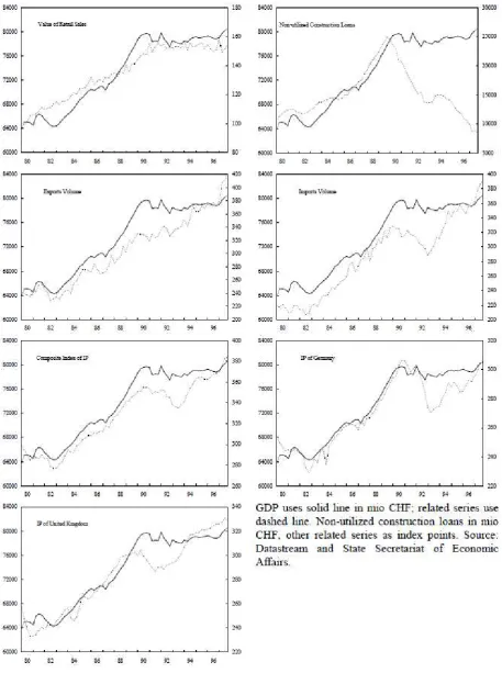
Tab. 2 provides the basic summary statistics of the quarterly and monthly series, which are used for the interpolation in Cuche, Hess (2000). Fig. 10 shows theGDP and related series in Cuche, Hess (2000).Tab. 3 presents the interpolation results in Cuche, Hess (2000).

25

Tab. 2. Data description, where GDP is the Gross Domestic Product, xrs is the value of retail sales to proxy for private consumption, xnl is the value of non-utilized construction loans to proxy for investment, xX is the value of exports, xM is the value of imports, xgip is the composite IP index of the Germany, xukip is the composite IP index of the UK, xcomip is the composite IP index of the

Switzerland, µ is the mean, σ is the standard deviation, AR(1) is the first order autoregressive coefficient, JB is the Jarque-Bera test, ADF is the augmented Dickey-Fuller test (after Cuche,

26

27

28

The application of the Stratonovich – Kalman – Bucy filtering algorithm and related scientific problems in the economics and finances have been researched in Athans (1974), Fernandez (1981), Geweke, Singleton (1981), Litterman (1983), Meinhold, Singpurwalla (1983), Engle, Watson (1983), Harvey, Pierse (1984), Engle, Lilien, Watson (1985), de Jong (1991), Doran (1992), Tanizaki (1993), Venegas, de Alba, Ordorica (1995), Hodrick, Prescott (1997), Krelle (1997), Cuche, Hess (2000), Durbin, Koopman (2000), Morley, Nelson, Zivot (2002), Bahmani, Brown (2004), Broto, Ruiz (2004), Fernàndez-Villaverde, Primiceri (2005), Fernàndez-Villaverde, Rubio-Ramirez (2005, 2007), Ozbek, Ozale (2005), Proietti (2006), Ochoa (2006), Horváth (2006), Cardamone (2006), Pasricha (2006), Bignasca, Rossi (2007), Dramani, Laye (2007), Paschke, Prokopczuk (2007), Roncalli, Weisang (2008), Proietti (2008), Osman, Louis, Balli (2008), Gonzalez-Astudillo (2009), Bationo, Hounkpodote (2009), Mapa, Sandoval, Yap (2009), Chang, Miller, Park (2009), Fernàndez-Villaverde (2010), Theoret, and Racicot (2010), Lai, Te (2011), Jungbacker, Koopman, van der Wel (2011), Proietti, Luati (2012a, b), Darvas, Varga (2012), Hang Qian (2012).

Stratonovich – Kalman – Bucy filtering algorithm for accurate

characterization of financial and economic time-series with use of

state-space model in Matlab: Gross Domestic Product

Let us begin with the consideration of the steady state filter and the time varying filter, which are designed and simulated in Matlab (R2012).

Problem description:

Let us use the following discrete plant: x(n+1) = Ax(n) + Bu(n),

y(n) = Cx(n) + Du(n), where

A = [1.1269 -0.4940 0.1129, 1.0000 0 0, 0 1.0000 0]; B = [-0.3832

29

D = 0.

Let us design the Stratonovich – Kalman – Bucy filter to estimate the output y based on the noisy measurements yv[n] = C x[n] + v[n]

The steady-state Stratonovich-Kalman-Bucy filter design:

Let us use the function KALMAN to design a steady-state Stratonovich – Kalman – Bucy filter. This function determines the optimal steady-state filter gain M based on the process noise covariance Q and the sensor noise covariance R. First, let us specify the plant + noise model. Let us set the sample time to -1 to mark the plant as discrete:

Plant = ss(A,[B B],C,0,-1,'inputname',{'u' 'w'},'outputname','y'). Let us specify the process noise covariance (Q):

Q = 2.3; % A number greater than zero.

Let us specify the sensor noise covariance (R): R = 1; % A number greater than zero.

Let us now design the steady-state Stratonovich – Kalman – Bucy filter with the equations:

Time update:

x[n+1|n] = Ax[n|n-1] + Bu[n], Measurement update:

x[n|n] = x[n|n-1] + M (yv[n] - Cx[n|n-1]), where M = optimal innovation gain, using the KALMAN command:

[kalmf,L,~,M,Z] = kalman(Plant,Q,R);

The first output of the Stratonovich – Kalman – Bucy filter KALMF is the plant output estimate y_e = Cx[n|n], and the remaining outputs are the state estimates. Let us keep only the first output y_e:

kalmf = kalmf(1,:); M, % innovation gain M =

0.5345 0.0101 -0.4776

30

Fig. 11.Stratonovich – Kalman – Bucy filter scheme (after Matlab (R2012).

To simulate the system above, let us generate the response of each part separately or generate both together. To simulate each separately, first let us use LSIM with the plant and then with the filter. The following example simulates both together.

% First, build a complete plant model with u,w,v as inputs and % y and yv as outputs:

a = A;

b = [B B 0*B]; c = [C;C]; d = [0 0 0;0 0 1];

P = ss(a,b,c,d,-1,'inputname',{'u' 'w' 'v'},'outputname',{'y' 'yv'});

Next, let us connect the plant model and the Stratonovich – Kalman – Bucy filter in parallel by specifying u as a shared input:

sys = parallel(P,kalmf,1,1,[],[]);

Finally, let us connect the plant output yv to the filter input yv. Note: yv is the 4thinput of SYS and also its 2nd output:

SimModel = feedback(sys,1,4,2,1);

SimModel = SimModel([1 3],[1 2 3]); % Delete yv form I/O

The resulting simulation model has w,v,u as inputs and y,y_e as outputs: SimModel.inputname

ans = 'w' 'v' 'u'

SimModel.outputname ans =

31

'y_e'

Let us simulate the filter behavior. Let us generate the sinusoidal input vector (known): t = (0:100)';

u = sin(t/5)

Let us generate the process noise and sensor noise vectors: rng(10,'twister');

w = sqrt(Q)*randn(length(t),1); v = sqrt(R)*randn(length(t),1);

Let us now simulate the response using LSIM: clf;

out = lsim(SimModel,[w,v,u]);

y = out(:,1); % true response ye = out(:,2); % filtered response yv = y + v; % measured response

Let us compare the true response with the filtered response: clf

subplot(211), plot(t,y,'b',t,ye,'r--'), xlabel('No. of samples'), ylabel('Output') title('Kalman filter response')

32

Fig. 12. Stratonovich – Kalman – Bucy filter response (after Matlab (R2012).

As shown in the 2nd plot in Fig. 12, the Stratonovich – Kalman – Bucy filter reduces the error y-yv due to measurement noise. To confirm this, let us compare the error covariances: MeasErr = y-yv;

MeasErrCov = sum(MeasErr.*MeasErr)/length(MeasErr); EstErr = y-ye;

EstErrCov = sum(EstErr.*EstErr)/length(EstErr);

The covariance of error before filtering (measurement error): MeasErrCov

MeasErrCov = 0.9871

The covariance of error after filtering (estimation error): EstErrCov

33

The time-varying Stratonovich-Kalman-Bucy filter design:

Let us design a time-varying Stratonovich – Kalman – Bucy filter to perform the same task. A time-varying Kalman filter can perform well even when the noise covariance is not stationary. However, in this demonstration, let us use the stationary covariance.

The time varying Stratonovich – Kalman – Bucy filter has the following update equations.

Time update:

x[n+1|n] = Ax[n|n] + Bu[n]; P[n+1|n] = AP[n|n]A' + B*Q*B'; Measurement update:

x[n|n] = x[n|n-1] + M[n](yv[n] - Cx[n|n-1]) -1 M[n] = P[n|n-1] C' (CP[n|n-1]C'+R) P[n|n] = (I-M[n]C) P[n|n-1]

First, let us generate the noisy plant response: sys = ss(A,B,C,D,-1);

y = lsim(sys,u+w); % w = process noise yv = y + v; % v = measurement noise

Next, let us implement the filter recursions in a FOR loop: P=B*Q*B'; % Initial error covariance

x=zeros(3,1); % Initial condition on the state ye = zeros(length(t),1);

ycov = zeros(length(t),1); errcov = zeros(length(t),1);

for i=1:length(t)

% Measurement update Mn = P*C'/(C*P*C'+R);

x = x + Mn*(yv(i)-C*x); % x[n|n] P = (eye(3)-Mn*C)*P; % P[n|n]

ye(i) = C*x;

34

% Time update

x = A*x + B*u(i); % x[n+1|n] P = A*P*A' + B*Q*B'; % P[n+1|n] end

Fig. 13. Time-varying Stratonovich – Kalman – Bucy filter response (after Matlab (R2012).

Now, let us compare the true response with the filtered response as shown in Fig. 13: subplot(211), plot(t,y,'b',t,ye,'r--'),

xlabel('No. of samples'), ylabel('Output')

title('Response with time-varying Kalman filter') subplot(212), plot(t,y-yv,'g',t,y-ye,'r--'),

xlabel('No. of samples'), ylabel('Error')

35

subplot(211)

plot(t,errcov), ylabel('Error Covar'),

title('Output covariance estimated by time-varying Kalman filter') subplot(212), plot(t,y-yv,'g',t,y-ye,'r--'),

xlabel('No. of samples'), ylabel('Error')

From the covariance plot in Fig. 13, it can be seen that the output covariance did reach a steady state in about 5 samples. From then on, the time varying filter has the same performance as the steady state version.

Let us compare the covariance errors: MeasErr = y-yv;

MeasErrCov = sum(MeasErr.*MeasErr)/length(MeasErr); EstErr = y-ye;

EstErrCov = sum(EstErr.*EstErr)/length(EstErr);

The covariance of error before the filtering (measurement error): MeasErrCov

MeasErrCov = 0.9871

The covariance of error after the filtering (estimation error): EstErrCov

EstErrCov = 0.3479

Let us verify that the steady-state and final values of the Kalman gain matrices coincide: M,Mn

36

Fig. 14. Output covariance estimated by time-varying Kalman filter (after Matlab (R2012).

short-37

run fluctuations” as explained in Osman, Louis, Balli (2008). We found that the Australia, Germany and the USA have the different business cycles, because the Australian and Germany economies are in the period of economic growth and the USA economy is in the contraction phase, caused by the economic recession.

Conclusion

38 Acknowledgement

39

and financial engineering. It is a real privilege for the second author to deliver his special personal thanks to Profs. Janina E. Mazierska, Electrical and Computer Engineering Department, James Cook University in Townsville in Australia, who helped us to cultivate the logical scientific thinking to tackle the complex scientific problems on the nonlinearities, applying the interdisciplinary scientific knowledge as well as the computer modeling skills. Finally, the authors thank the senior management team at The Mathworks for the license and kind permission to get a remote access to the software library with the different implementations of the Stratonovich – Kalman - Bucy filtering algorithm in the Matlab at the Mathworks servers in the USA.

40 References:

1. Menger C 1871 Principles of economics (Grundsätze der Volkswirtschaftslehre) Ludwig

von Mises Institute Auburn Alabama USA

http://www.mises.org/etexts/menger/Mengerprinciples.pdf .

2. von Böhm-Bawerk E 1884, 1889, 1921 Capital and interest: History and critique of interest theories, positive theory of capital, further essays on capital and interest Austria; 1890 Macmillan and Co edition Smart W A translator London UK http://files.libertyfund.org/files/284/0188_Bk.pdf .

3. von Mises L 1912 The theory of money and credit Ludwig von Mises Institute Auburn Alabama USA http://mises.org/books/Theory_Money_Credit/Contents.aspx .

4. von Mises L 1949 Human action Yale University Press USA Ludwig von Mises Institute Auburn Alabama USA http://mises.org/humanaction .

5. Hazlitt H 1946 Economics in one lesson Harper & Brothers USA.

6. Hayek F A 1931, 1935, 2008 Prices and production 1st edition Routledge and Sons London UK; 2nd edition Routledge and Kegan Paul London UK; 2008 edition Ludwig von Mises Institute Auburn Alabama USA.

7. Hayek F A 1948, 1980 Individualism and economic order London School of Economics and Political Science London UK, University of Chicago Press Chicago USA.

8. Rothbard M N 1962, 2004 Man, economy, and state Ludwig von Mises Institute Auburn Alabama USA http://www.mises.org/rothbard/mes.asp .

9. Hirsch M 1896, 1985 Economic principles: A manual of political economy The Ruskin Press Pty Ltd 123 Latrobe Street Melbourne Australia.

10. Bagehot W 1873, 1897 Lombard Street: A description of the money market Charles Scribner’s Sons New York USA.

11. Owen R L 1919 The Federal Reserve Act: Its origin and principles Century Company New York USA.

12. Willis H P 1923 The Federal Reserve System: Legislation, Organization, and Operation Ronald Press Company New York USA.

13. Mandel’shtam L I 1948-1955 Full collection of research works Publishing House of Academy of Sciences of the USSR vols 1 - 5 St Petersburg Moscow Russian Federation.

14. Wiener N 1949 The extrapolation, interpolation and smoothing of stationary time series John Wiley & Sons Inc New York NY USA.