Urbanization as a way of saving our planet from overpopulation

(1)

Munich Personal RePEc Archive

Urbanization as a way of saving our

planet from overpopulation

Shcherbakova, Nadezda

Saint Pteresburg state polytechnical university

November 2013

Online at

https://mpra.ub.uni-muenchen.de/52299/

(2)

1

Urbanization as a way of saving our planet from

overpopulation

Abstract

This paper explores whether biological mechanisms, induced by the overpopulation of a territory, exert essential influence on cities' growth, and whether the level of economic development of a country is significant, when biological mechanisms are in operation. To answer these questions, four hypotheses, based on the theoretical statements and empirical findings of ethology and demography, are formed. The results of regression analysis of statistical data on national level, applied to test these hypothesis, show that that biological factors should be considered as one of the determinants of cities' growth, but a complex analysis of factors of urban development is needed. The biological mechanisms of population reduction play a significant role in the least and less developed countries: with per capita GDP growth the concentration of population in big cities increases. Total fertility rate varies significantly in these countries, but with population growth it gradually decreases. In more developed countries with high per capita GDP level less than 60% of people live in cities with the population of 1 million inhabitants or more, and a total fertility rate stabilizes there at a simple reproduction level of ca. 2,0 births per woman.

Keywords: urbanization, overpopulation, fertility rate, birth rate, population density

1. Introduction

In urban economics the formation of cities and their growth are explained by the number of endogenous and exogenous factors, including an access to public good, scale and localization economies, economies due to product differentiation, multiplicative effect of industrial development, spatial advantages from locating near transport nodes. While biological, natural factors of urban development are mentioned in economic literature only collaterally.

However, the interdisciplinary approach to the problem of cities' growth, particularly relying on the knowledge from human ethology and demography, is also interesting and promises to be productive. Human ethology, studying the behaviour of humans as social animals, states that the main reason of cities' population growth is a scarcity of nature resources, overpopulation of our planet. The permanently worsening conditions of rural life force people to move to cities and towns. The biological mechanisms of population reduction lead to urbanization, which is a natural way of lowering population fertility. In their turn, demographers observe the lower fertility rates in cities in comparison with less densely populated areas.

Biological mechanisms often induce people to act against their economic interests and, as it would seem, in spite of common sense, but in economic literature they are considered as minor, not so essential, whereas economic incentives, cost-benefit ratio without backing on "basic instincts" of society are putted on the first place.

Thus, the theoretical statements of urban economics can be developed by adding a biological factor to the analysis of urban development. The overpopulation of a territory leads to cities' growth, and in cities the fertility rate of population reduces.

(3)

2 decreases. And another important question of this research is whether the level of economic development of a country plays an essential role, when biological mechanisms are in operation.

The paper is organized as follows. In Section 2, the main approaches from regional and urban economics, ethology, and demography which explain the urban growth with a glance to biological, natural factors are analysed. At the end of this section main hypotheses of the research are formed on the basis of results of the literature review. In Section 3, I describe statistical data and the main indicators, used in the course of the research. In Section 4, to test the suggested hypotheses the regression analysis is fulfilled. Finally, Section 5 contains the conclusions.

2. Literature Review

There are several approaches to the explanation of emergence and growth of towns and cities in regional and urban economics. Among them are conventional urban economics, the theory of industrial organization, the New Economic Geography, the theory of endogenous economic growth. The aim and tasks of this paper do not imply the elucidation of these theories, they are thoroughly described in many publications (e.g., see Abdel-Rahman and Anas, 2004).

However, in the context of this research it is worth pointing out that in economic literature biological, natural factors are mentioned only collaterally. Natural limitations are sometimes in question, when urban-rural linkages are considered. Because of shortage of working places, hunger through crop failures, drought in rural areas, many people have to move to towns, cities to find a job, better opportunities (Mabogunje, 1970; Goldsmith et al., 2004). This kind of cities' growth is especially common in developing countries.

At the same time, it was realized long ago that the emergence and the development of cities was impossible without the rise in agriculture surplus, generated by technological progress (Fujita and Thisse, 2002; Lindblad, 1991). Nowadays thanks to technological and scientific development only a few workers, engaged in agriculture, are enough to provide a lot of city dwellers with food. In the USA, where incomes are especially high in agriculture, farmers with their families make up 1% of the country population, but they supply the rest 99% of population with foodstuffs (Sachs, 2008).

These facts allow me to conclude that the redundancy of people in rural areas contributes to urban development. This idea was expressed by many theorists of regional economics, but not enough attention was given to it. It is considered as minor, not so essential, whereas economic incentives, cost-benefit ratio without backing on "basic instincts" of society, which often induce people to act against their economic interests and, as it would seem, in spite of common sense, are putted on the first place.

In ethology cities, especially the big ones, are considered as collapsing gatherings, which are a relatively harmless way of population size decrease (Dolnik, 2004). When population size achieves its critical value, the territory becomes densely populated, biological mechanisms of population reduction come into force. Some of them are especially severe: epidemics, the increase in aggression among individuals. Another mechanisms, including collapsing gatherings, imply more delicate reduction, coming into operation long before critical size of population is achieved.

(4)

3 The researches, studying the influence of high population density on animals' behaviour, were carried out on many representatives of animal world. Among them are rats (Calhoun, 1962), insects (for example, Mediterranean fruit fly (Carey et al., 1995)), birds (Wynne-Edwards, 1986). One of the first researches, dedicated to this topic, was an experiment on rats, executed by John B. Calhoun. Its results was published in 1962 (Calhoun, 1962). He discovered that overcrowding among rats leaded to pathological behaviour, showing itself in increased aggression, violation of sexual relations (same-sex relations, rapes of female individuals, simplification or total disappearance of marriage rituals), decrease in care for posterity. The essential consequences of high density were decline in birth rate and growth of death rate.

At the same time males with their females who managed to claim up to the top of the hierarchical ladder conducted a normal way of life. This means in some sense that hierarchy is able to soften the pressure of overcrowding and to increase environment capacity (Chauvin, 2009; Wynne-Edwards, 1986).

Calhoun’s work aroused a large resonance in scientific world and inspired many scientists to research the problem of overcrowding from different aspects up to the challenges of living in densely populated big cities and methods of avoiding them (Ramsden and Adams, 2009). Stimulated by Calhoun’s research, Jonathan Freedman began the first laboratory studies of crowding among human beings at Stanford University in the late 1960s (Freedman, 1975). He sought the correlation between density and a variety of pathologies similar to those found in Calhoun’s laboratory. His summarized that crowding per se did not automatically lead to pathological behaviour. We cannot solve modern urban and ecological problems by merely reducing the density at which we live, but population density contributes to these problems (Moore, 1999).

So one of the central questions of these researches is an applicability of results, acquired on animals, to human beings (Kurchanov, 2012). There are two opposite views on this problem. One scientists reckon that these deductions cannot be applied to human beings, because high concentration of individuals of social species, among which are humans, may not have detrimental effect (Chauvin, 1968). People as opposed to rats in Calhoun’s experiment are able to cope with overpopulation (Ramsden and Adams, 2009).

Other scientists, including the author of this paper, consider these results to be applicable to humans. As biological mechanisms operate out of consciousness, the features of behaviour in the conditions of high population density are peculiar not only to animals, but also to humans (Dolnik, 2004). Each physical contact of individuals of the same species, including human beings, provokes a secretion of a small amount of adrenaline. A human, as well as any other individual, is able to withstand a certain load (Lindblad, 1991).

Humans were not created to live in the huge conglomerations, numbering thousands of individuals. Our behaviour is adapted to work within small tribal groups, counting little less than about one hundred individuals (Morris, 2010). The behaviour, directed to the avoidance of excessive contacts, allows us to hold the number of our acquaintances in the limits necessary to our species.

In big cities initially healthy forms of human behaviour are rare. The life in big cities is full of stress. The accumulation of huge human masses in limited urban area causes aggression, conduces to isolation and indifference to a neighbour, unification and loss of individuality (Lorenz, 1974). No wonder that the prevalence of hypertension rose with urbanization (Cacioppo et al., 2000).

(5)

4 be, if in the condition of increased population density there are more people than social roles for them, only violence and destruction of social organization can follow.

However, the scientists, holding these opposite views, have undivided opinion that urban life also has a lot of advantages. When people get together in close urban communities, a surge of their mental abilities is observed. Another huge advantage of supertribal conditions is relative freedom in the choice of activities in the conditions of big cities (Morris, 1996).

There are also a lot of facts from demography which confirm the arguments in support of the applicability of results, acquired on animals, to human beings. The fact of abrupt fertility rate fall in cities accompanied by alienation and indifference to children is known for a long time (Kurchanov, 2012). Two competing hypotheses are elaborated to explain this fact: the compositional and the contextual (Kulu, 2013). The compositional hypothesis suggests that fertility levels vary between places simply because different people live in different settlements (e.g., the larger share of higher educated people, students, married people live in cities), whereas the contextual hypothesis suggests that factors related to immediate living environment are of critical importance. Immediate living environment in cities is formed by such factors as high costs for rising children, lack of opportunities for many couples to improve housing conditions, promotion of individual autonomy and self-actualisation, leading to individual choices, which usually mean fewer children.

There is a number of specialized researches at the country level which explore regional differences in fertility rates and factors, influencing on them: in Great Britain (Newell and Gazeley, 2012), in Nigeria (Ushie et. al., 2011), in Finland and other Northern European countries (Kulu, 2013), in the US (Fox and Myrskylä, 2011), in Switzerland (Bonoli, 2008), etc.

All these studies also indicate that fertility rate is influenced by a set of factors (female education and employment, age at entry into marital union, contraceptive use, family structure, housing conditions), in which urban and rural residents differ, but population density of a settlement is one of the most important among them. The more densely an area is populated, the lower the fertility rate is. And all these factors have mainly objective character and they are hardly controllable by a state policy on birth rate regulation (Bonoli, 2008).

Besides studies show that in many countries urban-rural fertility variation has decreased over time, but significant differences between various settlements persist (Kulu, 2013; Ushie et. al., 2011).

It is worth mentioning that a lot of developing countries is characterized by a high fertility rate even in urban areas, leading to rapid population growth. Earlier the high fertility rate was necessary for the compensation of a high infant mortality rate in these countries. But humanitarian aid to these countries promoted rapid infant mortality rate reduction, whereas the fertility rate needs more time to decrease in accordance with the reduced infant mortality rate. In sustainable populations fertility rate conforms to infant mortality rate (Dolnik, 2004).

At the same time Dolnik (2004) states that there is no strict dependence between poverty and fertility. "Poverty" and "wealth" are indistinct concepts even in economy and sociology. The strict causal relationship between such a subjective and short-term notion as poverty and such a long-term population answer as fertility rate cannot arise.

On the basis of the foregoing literature review the following conclusions can be drawn: 1. Though the influence of natural (including biological) factors on cities' formation and development is not denied in the urban economics theory, only minor importance is attached to them. The priority is given to economic incentives. However, under the influence of natural factors the behaviour of economic agents often happens to be irrational in terms of economic interests;

(6)

5 population. By the high population density fertility rate decreases, population size significantly reduces already to the second generation;

3. The possibility of applying the results of researches of animals' behaviour in the conditions of high density to human beings is called in question in academic circles, however, the fact of fertility rate decrease with population density growth is well-known from demography.

These conclusions allow me to form the following hypotheses, which are to be tested in the course of the study in order to define the level of influence of biological factor on cities' growth:

Hypothesis 1: Rapid urban growth, which is typical for countries with high birth rate, is induced by the overpopulation of a territory.

Hypothesis 2: Urbanization is a natural way of reducing population fertility. With the growth of urban population fertility rate reduces.

Hypothesis 3: There is no strict dependence between poverty (the level of social and economic development of a country) and fertility.

Hypothesis 4: In sustainable populations (we can assume that more developed countries can be sustainable populations in this sense), characterized by the conformation of birth rate to infant mortality rate, high concentration of individuals on a limited territory is unnatural. Overpopulation is typical for poor countries.

3. Data Description

To test abovementioned hypotheses statistical data of the United Nations and the World Bank by countries for 1990, 2000, 2010 years are selected for the analysis because of their availability and relative sufficiency. The coverage of the countries is as maximal as possible, but it is limited by existence of relevant data. The consideration of data for 1990, 2000 and 2010 years allows me to carry out the analysis of indicators in dynamics with an interval of 10 years. The choice of the years and the interval is also dictated by the existence of source data and the aim of the research.

With a view of testing the hypotheses of this research countries are classified by the level of economic development. Which countries can be characterized as being economically developed and which criteria are to be used are subjects of debate.

In the United Nations' statistical reports countries are divided by the level of economic development into the following groups:

1. More developed regions (comprise Europe, Northern America, Australia/New Zealand and Japan);

2. Less developed regions (all regions of Africa, Asia (excluding Japan), Latin America and the Caribbean plus Melanesia, Micronesia and Polynesia);

3. The least developed countries (48 countries, 33 in Africa, 9 in Asia, 5 in Oceania plus one in Latin America and the Caribbean);

4. Other less developed countries (the less developed regions excluding the least developed countries).

But this classification is made for statistical convenience and "do not necessarily express a judgement about the stage reached by a particular country or area in the development process"1.

In this research countries are divided into three groups by the level of per capita GDP at current prices.So far as GDP gradually grows in all countries of the world in the course of time, in 1990, 2000 and 2010 boundary values are different. So in 1990 the countries which are rated among more developed regions have per capita GDP more than 23000 US dollars. In less

1

(7)

6 developed regions per capita GDP varies between 4001 and 23000 US dollars. And the least developed countries have per capita GDP equal or less than 4000 US dollars.

In 2000 more developed countries have per capita GDP more than 25000 US dollars, less developed countries - more than 5000, but equal or less than 25000, and the least developed countries - equal or less than 5000.

In 2010 more developed countries have per capita GDP more than 46000 US dollars, less developed countries - more than 13000, but equal or less than 46000, and the least developed countries - equal or less than 13000.

Now we will pass to the step-by-step consideration of the indicators which are used to test the hypotheses, formed in the previous section.

To test the first hypothesis (sounding as follows: "Rapid urban growth, which is typical for countries with high birth rate, is induced by the overpopulation of a territory") the following indicators are considered:

- average annual rate of change of urban population by major area, region and country during previous five years, percent;

- birth rate, number of births per 1000 people; - urban population, percentage of total population; - population density, inhabitants per square kilometer;

- population of agglomerations with 1 million inhabitants or more, percentage of total population.

To test the second hypothesis (sounding as follows: "Urbanization is a natural way of reducing population fertility. With the growth of urban population fertility rate reduces") the following indicators are used:

- fertility rate, births per woman;

- urban population, percentage of total population.

To test the third hypothesis (sounding as follows: "There is no strict dependence between poverty and fertility") the following indicators are considered:

- fertility rate, births per woman;

- per capita GDP at current prices, US dollars.

And to test the fourth hypothesis (sounding as follows: "In more developed countries, characterized by the conformation of birth rate to infant mortality rate, high concentration of individuals on a limited territory is unnatural. Overpopulation is typical for poor countries") the following indicators are considered:

- population of agglomerations with 1 million inhabitants or more, percentage of total population;

- per capita GDP at current prices, US dollars; - birth rate, number of births per 1000 people;

- infant mortality rate, number of deaths per 1,000 people.

The sources of statistical information on values of these indicators are presented in Table 1.

Table 1. The sources of statistical information on values of the indicators, used for the analysis

Indicator Data source

Urban population, percentage of total population

Author's calculations on the basis of data of United Nations Statistics Division, UNSD Demographic Statistics (on-line at http://data.un.org)

Average annual rate of change of urban population by major area, region and country during previous five

(8)

7

Indicator Data source

years, percent (POP/ DB/WUP/Rev.2011)

Population density, inhabitants per square kilometer

United Nations Population Division, World Population Prospects: The 2010 Revision (on-line at http://data.un.org)

Population of agglomerations with 1 million inhabitants or more,

percentage of total population

United Nations, World Urbanization Prospects (on-line at: http://data.worldbank.org)

Fertility rate, births per woman The World Bank, World Development Indicators (on-line at http://data.un.org)

Birth rate (total, urban, rural), number of births per 1000 people

Infant mortality rate, number of deaths per 1,000 people

Per capita GDP at current prices, US dollars

United Nations Statistics Division, National Accounts Estimates of Main Aggregates (on-line at http://data.un.org)

Speaking about the construction of these indicators, it is worth giving definitions of the terms "fertility rate", "(crude) birth rate", and "infant mortality rate".

Fertility rate is a basic indicator of the level of fertility, calculated by summing age-specific birth rates over all reproductive ages. It may be interpreted as the expected number of children a women who survives to the end of the reproductive age span will have during her lifetime if she experiences the given age-specific rates2.

Crude birth rate is a number of live births, occurring among the population of a given geographical area during a given year, per 1000 mid-year total population of the given geographical area during the same year. It is a vital statistics summary rate based on the number of live births, occurring in a population during a given period of time, usually a calendar year3.

Infant mortality rate is a number of deaths under one year of age, occurring in a given geographical area during a given year, per 1000 live births, occurring among the population of the given geographical area during the same year. It is a vital statistics summary rate based on the number of infant, occurring during the same period of time, usually a calendar year4.

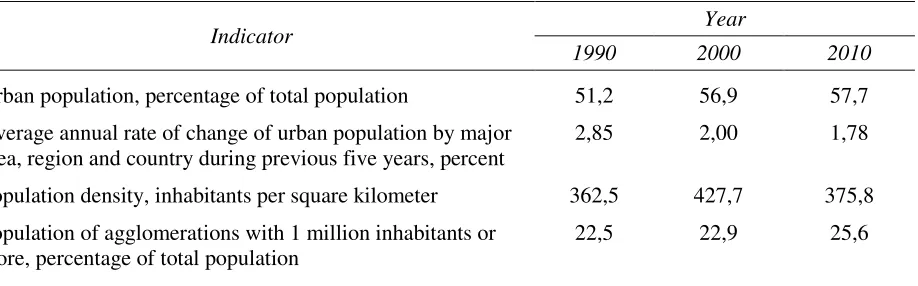
[image:8.595.98.557.569.712.2]

The dynamics of average values of the above listed indicators are shown in Table 2.

Table 2. Average values of the indicators

Indicator Year

1990 2000 2010

Urban population, percentage of total population 51,2 56,9 57,7

Average annual rate of change of urban population by major area, region and country during previous five years, percent

2,85 2,00 1,78

Population density, inhabitants per square kilometer 362,5 427,7 375,8

Population of agglomerations with 1 million inhabitants or more, percentage of total population

22,5 22,9 25,6

2

See Handbook on the Collection of Fertility and Mortality Data, United Nations, New York, 2004.

3

See Principles and Recommendations for a Vital Statistics System, Revision 2, United Nations, New York, 2001.

4

(9)

8

Indicator Year

1990 2000 2010

Fertility rate, births per woman 3,8 2,9 2,5

Birth rate, total, number of births per 1000 people 20,0 15,9 13,7

urban 18,8 13,5 13,3

rural 20,9 17,4 13,7

Average ratio of urban to rural birth rates 0,88 0,99 1,02

Infant mortality rate, number of deaths per 1,000 people 0,36 0,17 0,09

Per capita GDP at current prices, US dollars 6653,6 8788,3 16997,6

Notes: Author's calculations. The values were estimated over the countries over which there were data in the relevant year.

The analysis of dynamics of average values of the considered indicators reveals the following tendencies in the first approximation:

1. The share of urban population in total one increased, although its growth rate gradually reduced;

2. The concentration of population in big cities strengthened;

3. Against the background of increasing share of urban population fertility rate decreased; 4. Urban birth rate rose in comparison with rural birth rate. The share of countries with urban birth rate higher than rural one gradually increased from 29% in 1990 (41% in 2000) to 53% in 2010;

5. Both birth rate and infant mortality rate went down, but the ratio of birth rate to infant mortality rate increased significantly from 55,6 in 1990 to 152,2 in 2010;

6. Per capita GDP grew with increasing rates.

These tendencies bear some record to the first, to the second, and to the fourth hypotheses. At the same time the fourth tendency casts some doubt on the verity of the second hypothesis. In the next section to test thoroughly the above mentioned four hypotheses regression analysis with the usage of these indicators is carried out.

4. Empirical Analysis

To check the hypotheses of this research regression analysis is applied. One factor regression is taken into account. Among the types of models under consideration are simple regression models such as linear, exponential, square root, squared, logarithmic, reciprocal, multiplicative models and polynomial regression models (of the second order). Multiple regression models are not included in this paper, because all of considered models are reduced to one factor regression models in the course of the statistical analysis.

Most of the statistical calculations within the bounds of regression analysis are fulfiled with the help of the program "Statgraphics Centurion XVI.II".

(10)

9 at which the urban proportion is increasing. Both can be expressed in percentage terms. So the relations between the following indicators should be considered:

- the average annual rate of change of urban population of a country and its population density;

- the share of urban population in total population of a country and its population density; - the share of population of agglomerations with 1 million inhabitants or more and population density;

- the share of population of agglomerations with 1 million inhabitants or more in total population of a country and the share of its urban population;

- the average annual rate of change of urban population and a birth rate.

The regression analysis showed that there is a moderately strong relationship only between the last two variables in all considered years (see Table A1 in the Appendix A).

[image:10.595.124.514.299.527.2]

The moderately strong positive dependence between the share of urban population in total one and the share of population of agglomerations with 1 million inhabitants or more in total population of a country is observed. In 1990 and in 2000 this relation was exponential (Figure 1 and Figure 2, respectively). In 2010 the values of correlation coefficient and the coefficient of determination (R-squared) were maximal by squared-x model (Figure 3).

Figure 1. Dependence between the share of population of agglomerations with 1 million inhabitants or more in total population of a country and the share of urban population in 1990.

(11)

[image:11.595.111.524.59.286.2]

10

Notes: points - certain values for countries; thick solid line - an exponential trend line; thin solid line - confidence limits (confidence level = 95,0%); thin dashed line - prediction limits.

Notes: points - certain values for countries; thick solid line - trend line of the squared-x model; thin solid line - confidence limits (confidence level = 95,0%); thin dashed line - prediction limits.

[image:11.595.119.524.349.584.2]

(12)

11 in the residuals at the 95,0% confidence level. Selected regression models can be used to construct prediction limits for new observations.

Figures 1-3 depict that after crossing the threshold of 30% - 40% (percentage of urban population in total one) the percentage of population, living in urban agglomerations, in total population of a country starts to increase faster than before this level.

This dependence between the share of population of agglomerations with 1 million inhabitants or more and the share of urban population does not acquire any special traits by dividing the countries by the level of their economic development.

[image:12.595.122.522.229.465.2]

The second moderately strong positive relationship has been discovered between the average annual rate of change of urban population and a birth rate. In 1990 and in 2010 the best type of a model for this dependence was logarithmic (Figure 4 and Figure 6, respectively) and in 2000 - linear (Figure 5).

Figure 4. Dependence between the average annual rate of change of urban population in the period 1985-1990 and total birth rate in 1985-1990.

(13)

[image:13.595.115.524.56.286.2]

12

Notes: points - certain values for countries; thick solid line - trend line of the linear model; thin solid line - confidence limits (confidence level = 95,0%); thin dashed line - prediction limits.

Notes: points - certain values for countries; thick solid line - trend line of the logarithmic model; thin solid line - confidence limits (confidence level = 95,0%); thin dashed line - prediction limits.

[image:13.595.115.524.358.598.2]

(14)

13 The positive relationship between the average annual rate of change of urban population and a birth rate means that the higher birth rate is, the faster urban population grows in a country. But by the logarithmic models, showing the best values of statistical criteria in 1990 and 2010 years, there is a certain threshold of 17-20 births per 1000 people by which the average annual rate of change of urban population weakens its dependence on a birth rate.

If we divide countries by the level of economic development in the way described above, we shall see that this relation (including the above mentioned threshold) reveals itself better in the least developed countries of the world (see Table B1 in Appendix B). In these countries the average birth rate was equal 23 births per 1000 people in 1990, 18 births per 1000 people in 2000, and 16 births per 1000 people in 2010.

In less developed countries this positive correlation between a birth rate and the average annual rate of change of urban population is also observed, but this relationship is weaker. And the average total birth rate is smaller in these countries: it equalled 19 births per 1000people in 1990, 15 births per 1000 people in 2000, and 12 births per 1000 people in 2010.

In more developed countries the average birth rate stabilized at the level of 12-14 births per 1000 people in last twenty years. The average annual rate of change of urban population is positive in almost all more developed countries, but its dependence on total birth rate is not so strong as in other countries.

A logarithmic model is the most appropriate for this dependence in most cases. It implies the decrease in growth rates of the average annual rate of change of urban population in the range of large values of birth rate. This fact may be explained by a high level of infant mortality rate in the countries with a high level of birth rate.

To test the second hypothesis, saying that with the growth of urban population fertility rate reduces, relationship between fertility rate and the share of urban population in total population of a country is considered.

[image:14.595.116.523.463.682.2]

The regression analysis showed that there is a moderately strong relationship between these two variables in all considered years (see Table A2 in the Appendix A). In 1990 the best model, fitting this dependence, was a logarithmic model (Figure 7), in 2000 and in 2010 - a reciprocal-x model (Figure 8 and Figure 9, respectively).

Figure 7. Dependence between fertility rate and the share of urban population in total population of a country in 1990.

(15)

[image:15.595.122.518.57.271.2]

14

Notes: points - certain values for countries; thick solid line - trend line of the reciprocal-x model; thin solid line - confidence limits (confidence level = 95,0%); thin dashed line - prediction limits.

[image:15.595.124.516.342.560.2]

(16)

15 The moderately strong relationship between fertility rate and the percentage of urban population in total population of a country means that the more people live in cities and towns, the less children are born in it. But this dependence is not linear. After the threshold of ca. 40%-50% (percentage of urban population in total one) fertility rate gradually becomes stable at the average level of 2,0-3,0 births per woman.

The lack of relevant data does not allow me to fulfil the regression analysis of this relationship subject to the level of economic development of a country. But it is well observed that the stabilization at the average level of approximately 2,0-3,0 births per woman is more typical for less and more developed countries (see Figures C1-C3 in the Appendix C).

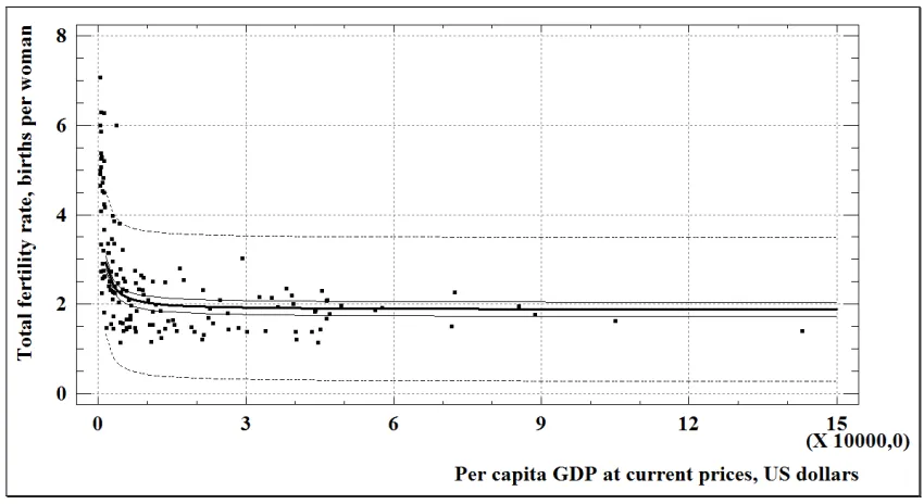
The third hypothesis states that there is no strict dependence between poverty (the level of social and economic development of a country) and fertility. To check this hypothesis the dependence between fertility rate and per capita GDP is considered. The results of regression analysis of this relationship are presented in the Appendix A (Table A2).

[image:16.595.114.526.284.506.2]

This analysis revealed a moderately strong relationship between these two variables. In 1990 the best fitted model for this dependence was a multiplicative model (Figure 10), in 2000 and in 2010 - a reciprocal model (Figure 11 and Figure 12, respectively).

Figure 10. Dependence between fertility rate and per capita GDP in 1990.

(17)

[image:17.595.116.523.56.271.2]

16

[image:17.595.106.531.331.563.2]

(18)

17 The moderately strong nonlinear relationship between these two indicators means that with per capita GDP growth fertility rate reduces till the definite level of ca. 1,5 - 2,5 births per woman.

According to the fourth hypothesis, in sustainable populations5, characterized by the conformation of birth rate to infant mortality rate, high concentration of individuals on a limited territory is unnatural. Overpopulation is typical for poor countries.

To check this hypothesis the relationships between the following variables will be considered:

- the share of population of agglomerations with 1 million inhabitants or more in total population of a country and its per capita GDP6;

- the ratio of birth rate to infant mortality rate and per capita GDP.

[image:18.595.112.531.257.490.2]

According to results of regression analysis, presented in Appendix A (Table A3), in all considered years a polynomial model of the second order fits the first dependence best of all (Figures 13-15).

Figure 13. Dependence between the share of population of agglomerations with 1 million inhabitants or more in total population of a country and its per capita GDP in 1990.

Notes: points - certain values for countries; thick solid line - trend line of the polynomial model of the second order; thin solid line - confidence limits (confidence level = 95,0%); thin dashed line - prediction limits.

5

It is assumed that more developed countries are sustainable populations in this sense. 6

(19)

[image:19.595.113.528.57.283.2]

18

[image:19.595.99.539.369.611.2]

(20)

19 model explains 23%-29% of the variability in the share of population of agglomerations. As the P-value of the Durbin-Watson statistic is greater than 0,05, there is no indication of serial autocorrelation in the residuals at the 95% confidence level. The P-value on the highest order term of the polynomial is less than 0,05, so the highest order term is statistically significant at the 95% confidence level.

The polynomial dependence between considered variables means that the highest concentration of population in big cities is more typical for less developed countries. In the least developed and more developed countries the share of population, living in urban agglomerations with 1 million inhabitants or more, is not so high as in less developed countries. In other words, at first with the growth of the level of economic development of a country the concentration of its population in big cities strengthens, but after achieving a certain level of per capita GDP (ca. 16000 US dollars in 1990, ca. 22000 US dollars in 2000, and ca. 36000 US dollars in 2010), this concentration gradually reduces.

[image:20.595.114.532.286.544.2]

The best trend line, fitting the dependence between the ratio of birth rate to infant mortality rate and per capita GDP, is also described by a polynomial model of the second order (Figures 16-17).

Figure 16. Dependence between the ratio of birth rate to infant mortality rate of a country and its per capita GDP in 1990.

(21)

[image:21.595.117.530.63.297.2]

20

[image:21.595.114.528.372.618.2]

(22)

P-21 value on the highest order term of the polynomial is less than 0,05, the highest order term is statistically significant at the 95% confidence level.

The polynomial model shows us that at first with per capita GDP growth the ratio of birth rate to infant mortality rate also increases, but after a certain value of per capita GDP (ca. 36000 US dollars in 1990, ca. 40000 US dollars in 2000, and ca. 90000 US dollars in 2010) it begins to decrease. In less developed countries this ratio is higher in comparison with the least and more developed countries. In the least developed countries this ratio is low because of the high infant mortality rate, and in more developed countries this ratio is comparatively low because of the low birth rate.

5. Conclusions

The aim of this research was to define the level of influence of the biological factor on cities' growth. In order to achieve this aim four hypotheses were put forward:

Hypothesis 1: Rapid urban growth, which is typical for countries with high birth rate, is induced by the overpopulation of a territory.

Hypothesis 2: Urbanization is a natural way of reducing population fertility. With the growth of urban population fertility rate reduces.

Hypothesis 3: There is no strict dependence between poverty (the level of social and economic development of a country) and fertility.

Hypothesis 4: In more developed countries, characterized by the conformation of birth rate to infant mortality rate, high concentration of individuals on a limited territory is unnatural. Overpopulation is typical for poor countries.

The results of the analysis of the dynamics of average values of the considered indicators (see Table 2) bearsome record to the first, to the second, and to the fourth hypotheses and at the same time cast some doubt on the verity of the second hypothesis.

To test these hypotheses more thoroughly the regression analysis was carried out. According to its results, the first, the second, and the fourth hypotheses are supposed to be proved. The fourth hypothesis is refuted.

The first hypothesis is considered to be provedowing to the discovered moderately strong positive dependence between the share of urban population in total one and the share of population of agglomerations with 1 million inhabitants or more in total population of a country. The exponential and squared-x forms of this relationship point out on its nonlinear nature: after crossing the threshold of 30% - 40% (percentage of urban population in total one) the percentage of population, living in urban agglomerations, in total population of a country starts to increase faster than before this level.

Undoubtedly, this hypothesis could be considered to be proved more grounded if the relationships between the average annual rate of change of urban population of a country and its population density and between the share of urban population in total population of a country and its population density had been discovered. But this research is fulfilled on a national level, and so the population density is considered only for a country as a whole. It is supposed that more detailed data on population density at a city level will reveal these dependences. Even on a national level, when city states are taken into consideration, the existence of these relationships is proved. For example, in extremely densely populated regions fertility rate is low. Among such areas are Monaco, Singapore and special administrative regions (of China) - Macao and Hong Kong, which can be considered as city states. Fertility rate in them does not exceed the level of 2,0 births per woman.

(23)

22

The second hypothesis is also considered to be proved. Such considerations rely on the discovered moderately strong relationship between fertility rate and the share of urban population in total population of a country. The more people live in cities and towns, the less children are born in it. But this dependence is not linear. After the threshold of ca. 40%-50% (percentage of urban population in total one) fertility rate gradually becomes stable at the average level of 2,0-3,0 births per woman. And this stabilization at the average level is more typical for less and more developed countries.

The third hypothesis is refuted thanks to the fulfilled regression analysis. The moderately strong nonlinear relationship between fertility rate and per capita GDP has been discovered in the course of this research. With per capita GDP growth fertility rate reduces till the definite level of ca. 1,5 - 2,5 births per woman. This observation allows me to argue with Dolnik (2004): the level of economic development of a country directly influences on its fertility rate. It is not the only factor, affecting fertility, but it is one of the determinative ones.

Finally, the fourth hypothesis is supposed to be proved. The regression analysis revealed the polynomial form (of the second order) of the dependence between the share of population of agglomerations with 1 million inhabitants or more in total population of a country and its per capita GDP. It means that in the least developed and more developed countries the share of population, living in urban agglomerations with 1 million inhabitants or more, is not so high as in less developed countries. The peak of concentration of population in big cities is observed at the mean level of economic development of a country.

Are more developed countries characterized by the conformation of birth rate to infant mortality rate, and can they be considered as sustainable populations? To answer these questions the dependence between the ratio of birth rate to infant mortality rate and per capita GDP was studied. It has been found out that this relationship is also better described by a polynomial model of the second order. In less developed countries this ratio is higher in comparison with the least and more developed countries. In the least developed countries high infant mortality rate compensates for high birth rate. But the swift decrease in infant mortality rate thanks to humanitarian aid led to unrestrained population growth in developing countries. And only more developed countries managed to find a new balance between birth rate and infant mortality rate. So more developed countries can be considered as sustainable populations in this sense.

The results of this research show that the biological factor should be considered as one of the determinants of cities' growth. But a complex analysis of factors of urban development is needed.

The biological mechanisms of population reduction play a significant role in the least and less developed countries: with per capita GDP growth the concentration of population in big cities increases. Fertility rate varies significantly in these countries, but with population growth it gradually decreases. In more developed countries with the high level of per capita GDP less than 60% of people live in cities with the population of 1 million inhabitants or more, and the fertility rate stabilizes at a simple reproduction level of ca. 2,0 births per woman7 in these countries.

It is worth emphasizing once more time that this research is fulfilled on a national level. The next step in studying the role of the biological factor in urban development will be a more detailed research on the level of a city.

Moreover, within the bounds of this research the notion of social and economic development of a country can be widened by adding some social and economic aspects such as per capita incomes, social security, life expectancy, etc. This can be an important contribution to this research, taking into account the current approach to GDP estimation. By this approach

7

(24)

23 service industries, which usually concentrate on urban areas, bring the biggest added value and so they make a considerable contribution in GDP formation.

References

Abdel-Rahman, H. M. and Anas, A. (2004) Theories of systems of cities, in: J. V. Henderson and J.-F. Thisse (Eds.) Handbook of Regional and Urban Economics, Volume 4: Cities and Geography, pp. 2293-2339. New York: Elsevier Science.

Bonoli, G. (2008) The impact of social policy on fertility: evidence from Switzerland, Journal of European Social Policy, 18(1), pp. 64-78.

Cacioppo, J. T., McClintock, M. K., Berntson, G. G. and Sheridan, J. F. (2000) Multilevel integrative analyses of human behavior: social neuroscience and the complementing nature of social and biological approaches, Psychological Bulletin, 126(6), pp. 829-843.

Calhoun, J.B. (1962) Population density and social pathology, Scientific American, 206(2), pp.139-150.

Carey, J.R., Liedo, P. and Vaupel, J.W. (1995) Mortality dynamics of density in the Mediterranean fruit fly, Experimental Gerontology, 30(6), pp. 605-629.

Chauvin, R. (1968) Animal Societies from the Bee to the Gorilla. New York: Hill & Wang. Chauvin, R. (2009) Povedenie jivotnih [Animals' behaviour]. Moscow: URSS: LIBROCOM. Dolnik, V. R. (2004) Neposlushnoe ditya biosfery. Besedy o povedenii cheloveka v kompanii ptits, zverey i detey [Disobedient child of the biosphere. Conversations about human behavior in the company of birds, beasts and children]. Saint-Petersburg: CheRo-na-Neve, Petroglif.

Fox, J., Myrskylä, M. (2011) Urban fertility responses to local government programs: evidence from the 1923-1932 U.S., Max Planck Institute for Demographic Research.

Freedman, J. L. (1975) Crowding and Behaviour. San Francisco: W. H. Freeman.

Fujita, M. and Thisse, J.-F. (2002) Economics of Agglomeration: Cities, Industrial Location, and Regional Growth. Cambridge: Cambridge University Press.

Goldsmith, P. D., Gunjal, K. and Ndarishikanye, B. (2004) Rural–urban migration and agricultural productivity: the case of Senegal, Agricultural Economics, 31(1), pp. 33–45.

Kulu, H. (2013) Why do fertility levels vary between urban and rural areas? Regional Studies, 47(6), pp. 895-912.

Kurchanov, N. A. (2012) Povedenie: evolucionniy podhod [Behaviour: evolutional approach]. Saint-Petersburg: SpecLit.

Lindblad, Y. (1991) Chelovek - ty, ya i pervozdannyj: Evoluciya cheloveka [Man - you, me and primeval: Human evolution]. Moscow: Progress.

Lorenz, K. (1974) Civilized Man's Eight Deadly Sins. London: Methuen & co.

Mabogunje, A. L. (1970) Systems approach to a theory of rural-urban migration, Geographical Analysis, 2(1), pp. 1–18.

Moore, J. (1999) Population density, social pathology, and behavioral ecology, Primates, 40(1), Special Edition: Primate Socioecology, pp. 1 - 22.

Morris, D. (1996) The Human Zoo: A Zoologist's Study of the Urban Animal. New York: Kodansha America, Inc.

Morris, D. (2010) The Naked Ape: A Zoologist's Study of the Human Animal. London: Random House.

Newell, A. and Gazeley, I. (2012) The declines in infant mortality and fertility: Evidence from British cities in demographic transition, Economics Department Working Paper Series, University of Sussex, No. 48-2012

Ramsden, E. and Adams, J. (2009) Escaping the laboratory: the rodent experiments of John B. Calhoun & their cultural influence, The Journal of Social History, 42(3), pp. 761-792.

Sachs, J. (2008) Common Wealth: Economics for a Crowded Planet. New York: Penguin Press. Ushie, M. A., Ogaboh, Agba A. M., Olumodeji, E. O. and Attah, F. (2011) Socio-cultural and economic determinants of fertility differentials in rural and urban Cross Rivers State, Nigeria, Journal of Geography and Regional Planning, 4(7), pp. 383-391.

(25)

24

[image:25.842.58.785.127.514.2]

Appendix A

Table A1. Results of regression analysis for testing the first hypothesis

Dependent variable (y) Independent

variable (x) Year

Maximal value of correlation

coefficient

Regression model R-squared, % T-statistic (P-value) F-ratio (P-value) Durbin-Watson statistic (P-value) Intercept Slope

Average annual rate of change of urban population during previous five years, percent

1990 -0,14 Square root-x model:

x y₌3,06₋0,02

1,8 15,9 (0,000) -1,9 (0,061) 3,6 (0,061) 1,5 (0,000)

x y=2,13−0,01

1,0 13,7 (0,000) -1,4 (0,160) 2,0 (0,160) 1,6 (0,001)

2010 -0,06 Reciprocal-x model:

x y=1,79−0,04

0,4 12,9 (0,000) -0,8 (0,450) 0,6 (0,450) 1,4 (0,000) Urban population, percentage of total population

x y=54,34−0,35

0,7 11,8 (0,000) -0,8 (0,450) 0,6 (0,450) 0,9 (0,000)

2000 0,05 Linear model:

x y₌56,35₋0,01

0,2 19,0 (0,000) 0,4 (0,670) 0,2 (0,670) 0,6 (0,000)

2010 -0,19 Logarithmic-x model:

x y₌68,58₋2,61ln

3,6 9,7 (0,000) -1,6 (0,110) 2,6 (0,110) 1,1 (0,000) Population of

agglomerations with 1 million inhabitants or more, percentage of total population

x y₌21,95₋0,13

0,2 8,0 (0,000) -0,5 (0,644) 2,2 (0,644) 1,3 (0,000)

2000 0,04 Squared-y model: ) 32 , 0 59 , 608 ( x

y= +

0,2 5,0 (0,000) 0,4 (0,670) 0,2 (0,670) 1,3 (0,000)

2010 0,24 Reciprocal-x model:

x y=21,70−67,30

(26)

25

Dependent variable (y) Independent

coefficient

Population of

agglomerations with 1 million inhabitants or more, percentage of total population

1990 0,66 Exponential model:

x

e y=5,62 0,02

43,2 9,9 (0,000) 6,6 (0,000) 43,4 (0,000) 1,7 (0,110)

2000 0,74 Exponential model:

x

e y₌4,84 0,02

55,3 9,8 (0,000) 8,5 (0,000) 72,8 (0,000) 2,1 (0,670)

2010 0,66 Squared-x model: 2 003 , 0 13 , 8 x

y₌ ₊

44,1 2,9 (0,006) 5,9 (0,000) 34,7 (0,000) 2,6 (0,980)

Average annual rate of change of urban population during previous five years, percent

Total birth rate, number of births per 1000 people

1990 0,51 Logarithmic-x model:

x y₌₋5,04₊2,32ln

26,1 -4,5 (0,000) 6,1 (0,000) 35,5 (0,000) 1,9 (0,230)

2000 0,58 Linear model:

x y₌₋0,83₊0,13

33,3 -2,9 (0,004) 7,9 (0,000) 62,5 (0,000) 2,0 (0,490)

2010 0,61 Logarithmic-x model:

x y=−4,52+2,18ln

(27)

[image:27.842.64.782.96.399.2]

26 Table A2. Results of regression analysis for testing the second and the third hypotheses

Dependent variable (y)

Independent

coefficient

Fertility rate, births per woman

1990 -0,70 Logarithmic-x model:

x y=12,09−2,21ln

48,5 12,6 (0,000) -8,8 (0,000) 78,3 (0,000) 1,9 (0,229)

x y=1,26−70,79

48,3 5,8 (0,000) 8,9 (0,000) 79,5 (0,000) 1,9 (0,231)

x y=1,14−68,79

32,5 3,9 (0,000) 5,7 (0,000) 32,2 (0,00) 2,0 (0,426)

Fertility rate, births per woman

1990 -0,74 Multiplicative model: 26 , 0 33 , 23 − = x y

54,7 22,2 (0,000) -13,9 (0,000) 194,1 (0,000) 1,5 (0,002)

x y=2,19+661,79

46,4 20,2 (0,000) 12,0 (0,000) 143,1 (0,000) 2,0 (0,392)

x y=1,88+1584,72

(28)

[image:28.842.58.798.104.373.2]

27 Table A3. Results of regression analysis for testing the fourth hypothesis

Dependent variable (y)

Independent

variable (x) Year Regression model

R-squared, % T-statistic (P-value) F-ratio (P-value) Durbin-Watson statistic (P-value) Constant Parameter

x

Parameter x2

Population of agglomerations with 1 million inhabitants or more, percentage of total population

1990 Polynomial model of the second order: 2 7 10 13 , 1 003 , 0 49 ,

13 x x

y −

⋅ − +

=

29,4 6,3 (0,000) 6,0 (0,000) -5,2 (0,000) 19,0 (0,000) 2,0 (0,469)

13 x x

y −

⋅ − +

=

29,0 6,6 (0,000) 4,5 (0,000) -3,1 (0,000) 19,4 (0,000) 2,3 (0,927)

14 x x

y −

⋅ − +

=

23,1 5,1 (0,000) 5,1 (0,000) -3,1 (0,003) 12,5 (0,000) 2,4 (0,964)

Ratio of birth rate to infant mortality rate, relative units

44 x x

y −

⋅ − +

=

60,3 7,6 (0,000) 5,9 (0,000) -2,7 (0,008) 63,0 (0,000) 1,7 (0,049)

56 x x

y −

⋅ − +

=

59,0 6,2 (0,000) 10,4 (0,000) -7,0 (0,000) 66,3 (0,000) 2,3 (0,865)

105 x x

y −

⋅ − +

=

(29)

28

[image:29.842.59.794.141.475.2]

Appendix B

Table B1. Results of regression analysis of the dependence between the average annual rate of change of urban population and total birth rate, divided by the level of economic development of a country

Year Level of economic development

Maximal value of

correlation coefficient Regression model

R-squared, %

T-statistic (P-value) F-ratio (P-value)

Durbin-Watson statistic (P-value) Intercept Slope

1990 The least developed countries

0,55 Square root-x model:

x y₌₋3,01₊1,08

30,5 -2,6 (0,012) 4,5 (0,000) 20,1 (0,000) 1,9 (0,347)

Less developed countries 0,41 Logarithmic-x model:

x y₌₋4,20₊2,02ln

16,6 -2,0 (0,057) 2,7 (0,010) 7,4 (0,010) 1,8 (0,253)

More developed countries 0,54 Square root-x model:

x y₌₋3,22₊1,16

29,4 -1,9 (0,076) 2,8 (0,011) 7,9 (0,011) 1,6 (0,176)

0,70 Logarithmic-x model:

x y₌₋6,98₊2,90ln

49,4 -6,1 (0,000) 7,1 (0,000) 49,9 (0,000) 2,4 (0,921)

Less developed countries 0,54 Logarithmic-x model:

x y₌₋3,62₊1,92ln

28,7 -2,9 (0,005) 4,2 (0,000) 17,3 (0,000) 1,6 (0,075)

More developed countries 0,52 Linear model:

x y=−0,26+0,11

27,5 -0,5 (0,623) 3,2 (0,004) 10,2 (0,004) 2,4 (0,832)

0,75 Logarithmic-x model:

x y=−6,02+2,66ln

55,5 -5,3 (0,000) 6,3 (0,000) 40,0 (0,000) 1,7 (0,189)

Less developed countries 0,55 Squared-x model: 2 005 , 0 25 , 0 x

y= +

30,4 0,9 (0,359) 3,5 (0,002) 12,2 (0,002) 1,7 (0,206)

More developed countries 0,48 Logarithmic-x model:

x y=−4,75+2,31ln

(30)

29

[image:30.595.126.513.78.283.2]

Appendix C

Figure C1. Dependence between fertility rate and the share of urban population in total population, divided by the level of economic development of countries, in 1990.

[image:30.595.132.510.363.570.2]

(31)

[image:31.595.136.509.61.265.2]

30