Sequential Tests for the Detection of Voice Activity and the Recognition of Cyber Exploits

Communications and Network, 2011, 3, 185-199

doi:10.4236/cn.2011.34022 Published Online November 2011 (http://www.SciRP.org/journal/cn)

Sequential Tests for the Detection of Voice Activity

and the Recognition of Cyber Exploits

*

Ehab Etellisi, P. Papantoni-Kazakos

Department of Electrical Engineering, University of Colorado Denver, Denver, USA E-mail:{ehababdalla.etellisi, Titsa.Papantoni}@ucdenver.edu

Received September 5, 2011; revised October 1, 2011; accepted October 19, 2011

Abstract

We consider the problem of automated voice activity detection (VAD), in the presence of noise. To attain this objective, we introduce a Sequential Detection of Change Test (SDCT), designed at the independent mixture of Laplacian and Gaussian distributions. We analyze and numerically evaluate the proposed test for various noisy environments. In addition, we address the problem of effectively recognizing the possible presence of cyber exploits in the voice transmission channel. We then introduce another sequential test, de-signed to detect rapidly and accurately the presence of such exploits, named Cyber Attacks Sequential De-tection of Change Test (CA-SDCT). We analyze and numerically evaluate the latter test. Experimental re-sults and comparisons with other proposed methods are also presented.

Keywords:Voice Activity Detection, Sequential Detection of Change Test, Cyber Exploits

1. Introduction

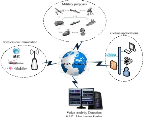
Voice Activity Detection (VAD) is deployed extensively, including the Global System for Mobile Communica-tions (GSM), as well as several satellite and radar mili-tary and civilian applications, (see in Figure 1). Thus, VAD is an important component of most systems that incorporate digital voice transmissions. During real time voice transmission, periods of voice activity are followed by silence, where both voice and silence periods are imbedded in background noise. Since voice is generally transmitted through fixed bandwidth links, the transmis-sion of the silence periods induces severe bandwidth waste. Voice Activity Detection (VAD) allows for the compression of the silence periods and may result in up to 30 to 40 percent of bandwidth savings.

To detect voice activity versus silence periods, the starting and ending points of continuous speech activity must be detected. Several research efforts have been in-vested in this area [1-3]. In this paper, we propose a novel VAD algorithm, named Voice Activity Detection using a Sequential Detection of Change Test (SDCT- VAD). The algorithm is designed at an independent mixture of Laplacian and Gaussian distributions; it is tracking effectively the boundary points between con-tinuous voice activity and silence time periods, where

during silence there is only noise, while during speech there is speech plus noise. The noise and noisy speech are modeled by a “Gaussian” versus “Laplacian plus independent Gaussian” distributions. Results are in-cluded for the cases where the SDCT-VAD is applied to detect voice activity, in both the presence and the ab-sence of noise. The algorithm is also tested within a real- time scenario, to exhibit its robustness and low complex-ity properties.

*_{Partially supported by the US Air Force Office of Scientific Research}

[image:1.595.309.539.515.703.2]

186

Considering the possibility of cyber exploits during voice transmission, we also present a novel cyber attack- sequential detection of change Test (CA-SDCT). The CA-SDCT algorithm is deployed during voice activity periods, as detected by the SDCT-VAD algorithm. The proposed CA-SDCA algorithm is designed at the Addi-tive White Gaussian Noise (AWGN) cyber attack model and is fully analysed and numerically evaluated in vari-ous environments.

The paper is organized as follows: In Section 2, the SDCT-VAD algorithm is presented. In Section 3, the CA-SDCT algorithm is developed. In Section 4, experi-mental results are included. In Section 5, we draw some conclusions.

2. Voice Activity Detection Algorithm

The general operation flowchart of the VAD algorithm is depicted by Figure 2. The problem to be solved here is the effective distinction between active and inactive voice periods. However, the variety of both the active voice and the ambient noise make this problem quite complicated in real life.

As shown in Figure 2, first the speech signal is gener-ated and is then corrupted by Additive White Gaussian Noise (AWGN). The AWGN affects the shapes of both the active voice and silence periods. The SDCT-VAD is then applied to detect voice activity periods. As will be further discussed in Section 3, the SDCT-VAD operates on various Signal-to-Noise Ratios (SNRs).

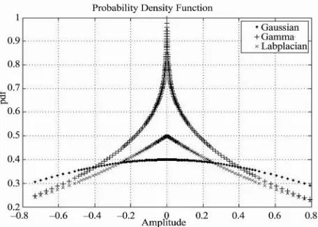
2.1. Speech and Noise Probability Distributions Throughout this section, we consider two distinct prob-ability density functions (pdfs) which represent the voice and noise amplitude distributions of the proposed model. The two distributions for speech and noise are assumed to be “Laplacian” and “Gaussian”, respectively, as in [4], where different speech distribution models are shown in Figure 3.

Figures 4-5 show noiseless and noisy actual speech signals, respectively.

To decrease algorithmic design complexity, we as-sume statistical independence between successive voice periods, as well as between signal and noise. We then derive the noisy speech distribution via the convolution of the Laplacian and Gaussian densities. Assuming that the corrupting noise is AWGN, the noisy speech signal is represented below,

signal AWGN

[image:2.595.308.537.81.465.2]

YX N (1) where Y denotes the noisy speech, _signal stands for the clean speech and N_AWGN represents the noise, and X

[image:2.595.310.538.505.668.2]

Figure 2. The general operation flowchart of the VAD algo-rithm.

Figure 3. Distributions voice signals.

signal and are statistically mutually

inde-pendent.

[image:3.595.71.274.87.259.2] [image:3.595.57.288.289.426.2]

187 E. ETELLISI ET AL.

Figure 4. Actual noiseless voice signal “silence + active voice”.

Figure 5. Actual voice “noisy voice signal”.

2.2. The Sequential Test for the Detection of Change

The sequential test for the detection of change, in its general form, was introduced and analyzed in [5-10]. It is assumed that an automated system will be monitoring the signal activity to decide when the voice is active versus not, whose design is based on the detection of change in the data generating stochastic process. The automated system will be implemented via the deployment of the SDCT-VAD algorithm which will be tracking voice to silence and silence to voice shifts, where voice and si-lence are modeled by two distinct stochastic processes. Below, we first present the general model considered in references [5-10].

Let and denote the n-dimensional density functions of two well known, distinct, mutually independent discrete-time stochastic processes at the vector point 1 2 n . Let it be known that

the active process is initially generated by the density function 0 [8]. For the problem addressed, it is

as-sumed that represents the noisy voice process, while

0 represents the AWGN noisy silence. Given the finite

sequence

 

n 0

f x

f

1

f

 

n 1

f x



,x ,



n

x  x , x

f



i



x x ;i 1 and the density functions

 

n

0

f x and

 

n 1

f x

δ

1

f

, the objective is to detect a possible

0 to f1 change as reliably and as quickly as possible.

To detect a possible such change, select some positive threshold . Then, observe data points sequentially and decide that thef0 to change has occurred the first

time such that f

n _{T x}

 

n _{δ, where}

 

 

n _{max 0,T x}



 

n1 _{g xn}

 

n



T 0 0 ; T x 

 

(2)

Where









i 1 1 i 1 i

i x l

g 

δ

f

i 1 0 i 1

x x x x





og f

f

The above algorithm operates sequentially via the use of two thresholds, 0 and , where 0 represents a re-flecting barrier and represents an absorbing or deci-sion barrier [8].

δ

f

When the two stochastic processes represented by the density functions 0 and 1 are memoryless, then the

conditioning in the log likelihood in (2) drops and the algorithmic operations are memoryless as well. A sym- metric algorithm that detects a shift from 1 to 0,

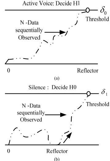
instead, can be easily derived. In Figure 6, the time- evolution of both algorithms is depicted.

f f

0



(a)

1



(b)

[image:3.595.331.510.414.675.2]

188

2.3. The SDCT-VAD Using Laplacian and Gaussian Distributions

Let and represent the density functions of a single datum x from noisy voice versus just noise, respectively. Let it be desirable to detect a possible change from

 

1

f x f x0

 

 

0

f x to f1



x



, where f x0

 

is Gaus- sian and 1 is Laplacian plus Gaussian. The as- sumption here is that the observed voice process is sta- tionary, memoryless and Laplacian, while the noise proc- ess is independent from the voice process and AWGN. Then,



f x



 



  

1 S N

f x 

_

_ f x y f y dy (3) where f x_S

 

is the Laplacian distribution that repre-sents the voice speech, and is the Gaussian dis-tribution representing the AWGN. N

 

f x

 



S

f x exp 2

a _{a x}

 



(4)

 

N

1

f x φ x

 

 

 _{ }

  (5)

where  denotes the standard deviation of the Gaus-sian distribution. We now derive the expressionf x1

 

:

 





1 1 x exp 2 a y

f a x y φ y

          _   _{  }    



 d



 





2

1 2

1

x exp exp

2 2π 2

a

d

y

f a x y y

           _   _      



Alternatively, the distribution f x1

 

can be expressed as follows,

 

2 2



   



1

f x exp

2 2

a a

h x h x



 

 _{ } 

   (6) where

 

exp





x

h x ax a



 

  _  _

 

 

exp

 

x

h x ax a



 

    _{ }

 

We then compute the log likelihood ratio updating step in the sequential test:

 

 

   





2 2 1 0 exp 2 2 log log 1

a a _{h x h x}

f x

x

f x _φ

                   _{ }     _{ }     

 

 

   





2 2 2

1 2 0 2π log In 2 2 In

f x a a

f x x

h x h x

 

The algorithmic updating step can be written as:

 

_In 2π 2 2 _In



   



2 2 2

g       h   h (7) where

 

exp



 



h      

The algorithmic step may be subsequently modified as follows

 

2π 2 2



   



In In

2 2 2

g  _   _  h  h

   (8)

where

; x

a

  



 

 

exp



 



h      

 

x x 1

 

u ud 





and

 

1 exp 2

2 2π

u

φ u _ _

 



and where the Signal to Noise Ratio (SNR) is:

2 2 2

2 2

SNR a

 

 

From the last equation, it can be recognized that the Signal-to-Noise Ratio (SNR) is a function of both the Laplacian constant and the standard deviation a of the noise. To develop a robust method for tracking the noise and speech signals, in Section 2.4, we will test the use of different SNRs in the design of the algorithm. In Figure 7, we plot the SNR as a function of , for various values of the standard deviation  of the noise.

Let us now select some positive threshold  and de-fine:

x



  

[image:4.595.299.542.105.387.2] [image:4.595.312.537.523.700.2]

189 E. ETELLISI ET AL.

2 2π ln 2 2 δ δ           

We may then modify the algorithm in (2), as mani-fested by the distributions derived in this section, via scaling, resulting in the following operation: Observe data sequentially and decide that the change from noise to voice activity has occurred the first time instant n such that _{T x}

 

n _δ , where

 

 

n



   

n 1

n

x max 0,T x  g xn



T 0 0 ; T x ma

 

 

   





1 2

n n 1

2

2π T x max 0,T x 1 ln ln

2 2

ln ln

2 h h

   _{ }    _       _               ₍₁₀₎

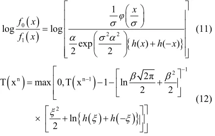
We note that the algorithm in (10) detects change from silence to active voice. The algorithm that detects change from active voice to silence, instead, is similarly derived, where its recursively derived algorithmic values are given by the expression in (12) below and where its de-cision threshold is generally different than that of the algorithm in (10).

 

 

_

_

0 2 2 1 1 log log

exp ( ) ( )

2 2

x

φ

f x f x

h x h x

      _{ }  _{ }     _                  (11)

 

 

   





1 2

n n 1

2

2π

T x max 0,T x 1 ln

2 2

ln

2 h h

   _{ }    _       _      _    _      (12)

2.4. Power and False Alarm Curves for Threshold Values Selections

In this section, we present algorithmic performance cri-teria and their use in the selection of the decision thresh-olds. We specifically evaluate power and false alarm curves induced by the two algorithms in Section 2.3 for several given decision thresholds. We then compare such curves for different threshold values, to subsequently de- cide on the values of the operational algorithmic thresh- olds. Let us define,

 f_ni

 

ξ ξd : The probability that at time n the algo-rithm has not crossed the threshold, δ, and its value lies in



ξ ξ, dξ



, given that the acting pdf is fi;

where, the recursive expression below can be derived,

 

 

n



n,i n 1,i S

x 0 /

f f x f

x

ξ ξ

 

   



_

 x dx



(13)

 The probabilities



βn; n 1



represent a power set,  The probabilities



αn; n 1



represent a false alarm

set.

The main objective here is to find the threshold that induces low false alarm and high power for small sample sizes. To compute the power and false alarm curves, as induced by the probability sequences



βn;n≥1



and



αn;n≥1



, respectively, we need to

analyse the characteristics of the updating step shown in Equation (8). This process is explained in the Appendix, where the expressions for the computation of the se-quences



β_n;n≥1



and α_n;n≥1



δ

are also derived. Given threshold , the silence mode to active voice mode change detecting algorithm is basically character-ized by two time curves: the power and false alarm curves, denoted respectively βn and , respectively,

where n denotes time instant and where, n

α

n

β : The probability that the silence to active voice mode change detecting algorithm crosses its threshold before or at time n, given that the operation mode is ac-tive voice mode throughout [6].

n: The probability that the silence to active voice

mode detecting algorithm crosses its threshold before or at time n, given that the operational mode is silence mode throughout [6].

α

When the algorithm that monitors change from mode silence to mode voice is considered, the threshold  may be selected based on the following principle: At given time n , have the powers induced by the parallel algorithms be above a predetermined lower bound, while the false alarm induced by each algorithm remains below a predetermined upper bound. The threshold for the al-gorithm that monitors change from voice to silence, in-stead, is selected similarly.

[image:5.595.70.290.392.531.2]

In Figure 8, we depict the βn and αn representative

190



curves, to observe and discuss qualitative characteristics. We plot these curves for two different threshold values. From the figure, we note that as the value of the decision threshold increases, the false alarm curve decreases, but so does the power curve. The threshold selection for the silence to active voice change monitoring algorithm may be based on a required lower bound for the power and a required upper bound for the false alarm, at a given time instant n. A similar criterion may be adopted in the threshold selection for the active voice to silence moni-toring algorithm.

3. An Algorithm for Detecting Cyber

Attacks during Speech Activity

In this section, we consider the case where the voice transmission channel may be vulnerable to cyber exploits. We then focus on developing an automated system that, in concurrence with voice activity detection, also detects cyber exploit activities. We thus develop a Cyber Attack- Sequential Detection of Change Test (CA-SDCT), de- signed to detect cyber attacks during voice activity peri- ods, as the latter are detected by the SDCT-VAD algo- rithm in Section 2. The block diagram of the overall sys- tem is depicted in Figure 2, Section 2. As shown in Fig- ure 2, first the speech signal is generated and is then corrupted by additive white Gaussian noise (AWGN). The SDCT-VAD is then deployed to distinguish between voice activity and silence periods. We finally wish to detect possible cyber attacks during voice activity periods.

As in Section 2.2, let and denote the n-dimensional density functions of two well known, dis-tinct, mutually independent discrete-time stochastic processes at the vector point 1 2 n . For the problem addressed here, 1 represents the process of

cyber exploits superimposed on noisy voice activity, while 0 represents the noisy voice activity process in

[image:6.595.332.510.83.326.2]

the absence of cyber attacks. Given the infinite sequence , let the n-dimensional density functions be denoted and 1 . The objective is to detect a possible ₀ to ₁ change as reliably and as quickly as possible, utilizing the observed data sequences. The sequential operation of the two algorithms is depicted in Figure 9.

n 0 f (x )

n x = f

n x )

n 1 f (x )

,x , ,x

{x }

f



i;i x= x 1

0 f (

f n

x ) f ( f

As in Section 2.2, we first select some positive thresh-old 0. Subsequently, we observe noisy voice data

se-quentially, during voice activity periods detected by the SDCT-VAD, and decide that the 0 to change has

occurred, the first time such that f f1

 

n

n T x 0, where

 

 

n



   



n

T 0 0 : T x max 0, T xn 1 g xn ₍₁₄₎

where

0 

(a)

1 

[image:6.595.311.540.559.658.2]

(b)

Figure 9. Making the final decision in the first crossing to the threshold. (a) Cyber Exploits Present, denoted H1; (b) Cyber Exploits Absent, denoted H0.

 

_i 1



_

11



_

i ₁

0 1

g x log

i i

i i

f x x f x x







A similar algorithm may be devised for the detection of shifts from 1 to , instead. 0

We model the presence of cyber exploits by Additive White Gaussian Noise (AWGN) that is superimposed on the transmission channel AWGN, resulting in relatively excessive cumulative white noise. When the two sto-chastic processes represented by the density functions

0 and 1 are memoryless, the conditioning in the log

likelihood in (14) drops and the algorithmic operations are memoryless as well. As directly deduced from Sec-tion 2.3, in the present case we have:

f f

f f

 



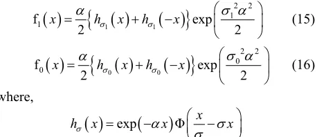
1

 

1

 



2 2

1 1

f e

2 2

x  h_ x h_ x xp_  

  (15)

 



0

 

0

 



2 2

0 0

f e

2 2

x  h_ x h_ x xp_  

  (16)

where,

 

exp





Φ x

h x  x _ x

 

0

 : Standard deviation of the transmission noise, in the absence of cyber exploits.

1

E. ETELLISI ET AL. 191 Then,

 

 

 

 





 

 





1 1 0 0 2 2 1 1 2 2 0 0 exp

f 2 2

log ln

f

exp

2 2

h x h x

x x

h x h x

              _{ }        _{ }   or,

 

 

 

 





 

 



01 10



2

1 2 2

1 0

0

f

log ln

f 2

h x h x

x

x h x h x

 

 

    

 

 _  _

  (17)

sen in the SDCT-VAD design are the Laplacian parame-ter, the standard deviation of the Gaussian noise and the two algorithmic thresholds: A threshold 0 used by the

algorithm in (10); for the detection of change from noise to noisy voice activity, and a threshold ₁ used by the

12); for the detection of change from noisy active voice to just noise. We used the power and false alarm curves discussed in Section 2.4, to decide on the s of these two thresholds. In particular, we selected

, , ,

δ

δ

algorithm in (

value

the (δ0 δ1 α  ) values (0.3, 0.05, 0.98, 0.0523).

We used the design parameter values (0.3, 0.05, 0.98, 0.0523) and tested the robustness of the resulting SDCT-VAD algorithm in the presence of various noisy environments. Various noises were mixed with the clean speech signals. Six different noises were used in our evaluations, including white noise, wind, computer fan, babble, flowing traffic and train passing. Figure 11 ex- The implementation of the cyber exploits detection

algo-rithm is then as follows:

During voice activity periods, as detected by the SDCT- VAD algorithm, observe data sequentially and decide that the change from absence to presence of cyber ex-ploits has occurred, the first time instant n such that

 

n 0

T x  , where Equation (18). hibits the various noise types, while Figures 12 and 13 show the effect of such noises when superimposed on the original noisy speech signal in Figure 10.

We note that the algorithm in (18) detects a to change. The algorithm that detects a to f0 change,

instead (from presence to absence of cyber exploits), is similarly derived, where its recursively derived algo-rithmic values are given by the expression in (19) below and where its decision threshold, 1

0

f f1

1

f

 is generally dif-ferent than that of the algorithm in (18), as shown in Figure 9.

For comparison, the same voice and noise environments are also tested by the approach presented in [2] and the G.729 VAD algorithm in [11]. The results are summarized in Tables 1 and 3. The noise data are obtained from http://www.freesound.org/index.php and are added to the clean speech signal at SNRs varying from 5 dB to 25 dB.

4. Experimental Results

4.1. Testing the SDCT-VAD

In this section, we state the steps involved in the nu-merical evaluation of the SDCT-VAD algorithm. First, we select the pertinent involved parameters and deploy the resulting SDCT-VAD algorithm, to detect any voice activity in the communication link. Then, the SDCT- VAD is evaluated in various noisy environments. In our simplified model, the silence plus noise mode of opera-tion is assumed to be represented by a Gaussian distribu-tion, while the noisy voice signal is represented by a mixture of Laplacian and Gaussian distributions, as

shown in Figure 10. The pertinent parameters to be cho- Figure 10. Original voice signal.

 







 

 



 

 



10 10



2

2 2

1 0

max 0, 1 ln

2

h x h x

T n T n

h x h x

           _    _   _  _   

 _ (18)

 







 

 



 

 



01 10



2

2 2

0 1

max 0, 1 ln

2

h x h x

T n T n

h x h x

           _{  }  _   _  _   

[image:7.595.55.289.92.215.2] [image:7.595.310.538.422.592.2]

[image:8.595.295.535.85.288.2]

192

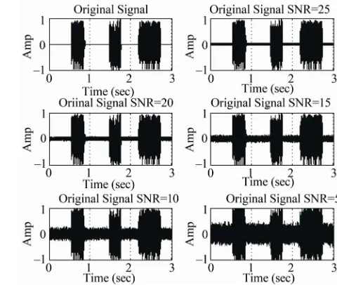
[image:8.595.58.289.85.292.2]

Figure 11. Various noisy environments. Figure 12. Original signal corrupted by AWGN “SNR = 25, _{20, 15, 10 and 5 dB”.}

[image:8.595.99.499.324.673.2]

193 E. ETELLISI ET AL.

To empirically evaluate the SDCT-VAD algorithm, many audio messages were used, with different lengths, (3 sec and 50 sec), with both male and female speakers and with different SNRs, (5 dB - 25 dB). The effect of these SNRs on the audio messages is exhibited in Figure 12, where Figure 10 exhibits the original speech signal.

To empirically evaluate the SDCT-VAD algorithm, many audio messages were used, with different lengths, (3 sec and 50 sec), with both male and female speakers

and with different SNRs, (5 dB - 25 dB). The effect of these SNRs on the audio messages is exhibited in Figure 12, where Figure 10 exhibits the original speech signal.

[image:9.595.140.462.455.705.2]

Figures 14 and 15 below show results for the SDCT- VAD algorithm with operating parameters as those stated in this Section, when the SNR is 25 dB and 5 dB, respectively. The accuracy of the results depends on the level of the SNRs and the type of the noise environment, as shown in Tables 1 and 2.

Figure 14. SDCT-VAD results “original voice signal corrupted by AWGN (SNR = 25 dB)”.

194

The efficiency of the SDCT-VAD algorithm was evaluated for various noisy voice signals. In the first ex-periment, we tested the efficiency of the proposed method using the same audio recording discussed above, tracing the speed and the accuracy of the algorithm in detecting the silence mode to active mode change and vice verse.

[image:10.595.308.539.242.705.2]

To comparatively evaluate the performance of the proposed SDCT-VAD algorithm, we compared its in-duced results with those of the manual segmentation. Figure 10 exhibits the “hand-marked” results of manual segmentation. Figures 14 and 15 exhibit the automated segmentation induced by the SDCT-VAD proposed al-gorithm. We evaluated the algorithmic probability of error (Pe), using the formula below:

 





_



_















2

1

2

_

_

N e Av

n

n

n

AVSP manual AVSP RSDC VAD P

AVSP manual

AVEP manual AVEP RSDC VAD AVEP manual



 _ 

 



 

 

 

 

 

 





(20)

AV: Active Voice;

AVSP: Active Voice Starting Point; AVEP: Active Voice Ending Point; N: Number of Active Voice Regions.

The performance of the SDCA-VAD is evaluated in terms of probability of false and correct decisions, where

cis the probability of correct speech classification and

where e, is the probability of false speech

classifica-tion, computed as in (20).

P P

Table 1. Comparing the starting and ending detection time instances of the noisy active voice messages using the man-ual and proposed method.

Message 1 Message 3 Message 3 SNR (dB)

AVSP AVEP AVSP AVEP AVSP AVEP

Manual 0 0.5294 0.8904 1.472 1.769 2.19 2.75

25 0.5295 0.8902 1.472 1.769 2.19 2.739

20 0.5298 0.8710 1.472 1.769 2.19 2.75

15 0.5356 0.870 1.472 1.769 2.19 2.75

10 0.5414 0.8695 1.472 1.769 2.19 2.75

Automatic RSDCA

-VAD

5 0.5366 0.8654 1.472 1.769 2.184 2.75

To compute ewe start with known voice activity and

the starting and ending points of voice activity marked. We then superimpose AWGN voice contamination with various SNRs (25, 20, 15, 10 and 5 dB) and deploy the corresponding SDCT-VAD for various noisy environ-ments, as shown in Figures 11-13. Results comparing the SDCT-VAD with the manual approach are shown in Table 1.

P

In Figures 16 and 17 we plot the and results

included in Table 2. c

[image:10.595.307.537.249.691.2]

P Pe

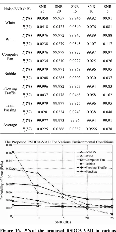
Table 2. PC's and PF's of the proposed RSDCA-VAD

for various environmental conditions.

Noise/SNR (dB) SNR ₂₅ SNR ₂₀ SNR ₁₅ SNR ₁₀ SNR ₅

(%)

c

P 99.958 99.957 99.946 99.92 99.91

White (%)

e

P 0.0418 0.0423 0.0540 0.076 0.081

(%)

c

P 99.976 99.972 99.945 99.89 99.88

Wind (%)

e

P 0.0238 0.0279 0.0545 0.107 0.117

(%)

c

P 99.976 99.979 99.977 99.97 99.97

Computer

Fan _(%)

e

P 0.0234 0.0210 0.0227 0.025 0.026

(%)

c

P 99.979 99.971 99.969 99.96 99.95

Babble (%)

e

P 0.0208 0.0285 0.0303 0.030 0.037

(%)

c

P 99.996 99.982 99.953 99.94 99.83

Flowing Traffic _(%)

e

P 0.0037 0.0178 0.0468 0.058 0.162

(%)

c

P 99.979 99.977 99.975 99.96 99.95

Train

Passing _(%)

e

P 0.020 0.0224 0.0243 0.038 0.048

(%)

c

P 99.977 99.973 99.96 99.94 99.91

Average (%)

e

[image:10.595.59.287.266.392.2]

P 0.0225 0.0266 0.0387 0.0556 0.078

[image:10.595.55.285.516.719.2]

[image:11.595.59.285.82.265.2]

195 E. ETELLISI ET AL.

Figure 17. P_c's of the proposed RSDCA-VAD in various environmental conditions.

To further validate the effectiveness of the proposed SDCT-VAD, we compared its probabilities of correct speech activity detection with those of other approaches. Table 3 shows a comparison between the SDCT-VAD and two different VAD approaches: the G.729 in [11] and the proposed method in [2].

The clean speech signal that has length of 50 sec, 60.05% speech and 39.95% silence, was used to evaluate

the proposed algorithm against various environmental conditions and to compare it with the ITU standard G729 Annex B [11] and the proposed in [2] approaches.

From Table 3, it can be recognized that even with en-vironmental challenging conditions, the proposed SDCT- VAD outperformed the G729B VAD and the method in [2].

4.2. Testing the CA-SDCT

As stated in Section 3, to detect shifts from absence to presence of cyber exploits and vice versa using the CA-SDCT algorithm, two algorithmic decision thresh-olds are needed: A threshold 0 used by the algorithm

in (18); for the detection of change from Cyber exploits absent to Cyber exploits present, and a threshold ₁ used by the algorithm in (19); for the detection of change from Cyber exploits present to Cyber exploits absent. It is assumed that the cyber attack is represented by AWGN. We tested the original signal and its noisy ver-sions, as those exhibited in Figure 18. Using the power and false alarm curves, as with the SDCT-VAD algo-rithm, we selected the pertinent thresholds. In particular, we selected the ( 0,δ1, , 1

δ

δ

δ α  ) design values (0.07, 0.01, 0.98, 0.0773), while we tested the 2 values (0.0798,

[image:11.595.56.539.439.725.2]

0.0849, 0.1034), to evaluate the robustness of the result-ing CA-SDCT algorithm.

Table 3. P_c's of the proposed RSDCT-VAD, and different VAD approaches for various environmental conditions.

Environment G.729 VAD _[2,11] Proposed Method in [2] Proposed RSDCA-VAD

Noise SNR P_c(%) P_c(%) P_c(%)

5 87.46 75.62 97.563

15 97.83 93.42 99.136

White

25 99.69 99.07 99.328

5 97.29 97.83 98.131

15 99.77 99.46 99.711

Vehicle

25 100.00 100.00 99.781

5 92.96 86.38 97.201

15 98.45 94.89 99.504

Babble

196

(a) (b)

(c) (d)

Figure 18. (a) Original signal; (b) Noisy signal with SNR = 15 dB; (c) Noisy signal with SNR = 10 dB; (d) Noisy signal with SNR = 5 dB.

(a) (b)

[image:12.595.69.531.82.352.2]

(c)

[image:12.595.95.504.387.691.2]

E. ETELLISI ET AL. 197

(a) (b)

[image:13.595.95.507.82.452.2]

(c)

Figure 20. Cyber detection during speech activity detected periods using RSDA-CA. (a) Alarms SNR = 15; (b) Alarms SNR = 10; (c) Alarms SNR = 5.

From Figure 19, parts (a), (b) and (c), we may observe the evolution of the deployed CA-SDCT algorithm for different SNR values, where the latter values reflect the cumulative effect of normal channel noise and cyber noise. Each time the threshold is crossed, an alarm is activated.

Figure 20 shows alarm activation scenarios regarding cyber attacks, where in (a) no alarm is activated, where in (b) one alarm is activated and where in (c) several alarms are activated.

5. Conclusions

A novel voice activity detection (VAD) approach was presented. The approach uses the Sequential Detection of Change Algorithm (SDCT-VAD), designed at the Lapla-cian-Gaussian distributions additive mixture. We ana-lysed and evaluated the robust sequential algorithm in the presence of Additive White Gaussian Noise. Several

different speech messages were chosen for the effective-ness evaluation of the SDCT-VAD, regarding its accu-rate detection of changes from voice activity to silence and vice versa. The experimental results have shown that the algorithm is effective in various noisy environments and outperforms other existing voice activity detection methods.

198

Additive White Gaussian Noise. The experimental re- sults have shown how the algorithm can be implemented with effective detection results, in a variety of different environments.

6. References

[1] J.-W. Shin, H.-J. Kwon, S.-H. Jin and N. S. Kim, “Voice Activity Detection Based on Conditional MAP Crite-rion,” IEEE Signal Processing Letters, Vol. 15, 2008, pp. 257-260.

[2] J. Sohn, N.-S. Kim and W.-Y. Sung, “A Statistical Model-Based Voice Activity Detection,” IEEE Signal Processing Letters, Vol. 6, No. 1, 1999, pp. 1-3.

[3] J.-W. Shin, J.-H. Chang, H.-S. Yun and N.-S. Kim, “Voice Activity Detection Based on Generalized Gamm Distribution,” Vol. 1, 2005, pp. 781-784.

[4] S. Gazor and W. Zhang, “Speech Probability Distribu-tion,” IEEE Signal Processing, Vol. 10, No. 7, 2003, pp. 204-207. doi:10.1109/LSP.2003.813679

[5] R. K. Bansal and P. Papantoni-Kazakos, “An Algorithm for Detecting a Change in a Stochastic Process,” IEEE Transac-tion on InformaTransac-tion Theory, Vol. IT-32, No. 2, 1986, pp.

227-235.

[6] A. T. Burrell and P. Papantoni-Kazakos, “Extended Se-quential Algorithms for Detecting Changes in Acting Stochastic Processes,” IEEE Transaction on Systems,

Man, and Cybernetics,Vol. 28, No. 5, 1998, pp. 703-710. doi:10.1109/3468.709621

[7] A. T. Burrell and P. Papantoni-Kazakos, “Detecting Soft-ware Faults in Distributed Systems,” IEEE 2009 World Congress on Computer Science and Information Engi-neering, Vol. 7, 2009, pp. 300-304.

[8] P. Papantoni-Kazakos, “Algorithms for-Monitoring Changes in Quality of Communication Links,” IEEE Transaction on Communication, Vol. COM-27, 1979, pp. 682-692. [9] D. Kazakos and P. Papantoni-Kazakos, “Detection and

Estimation,” Computer Science Press, New York, 1990. [10] P. Papantoni-Kazakos, “Algorithms for Monitoring Changes

in Quality of Communication Links,” IEEE Transactions on Communication, Vol. COM-27, 1979, pp. 656-659. [11] A. Benyassine, E. Shlomot, H.-Y. Su, D. Massaloux, C.

Lamblin and J.-P. Petit, “ITU-T Recommendation G.729 Annex B: A Silence Compression Scheme for Use with G.729 Optimized for V.70 Digital Simultaneous Voice and Data Applications,” Communications Magazine, IEEE, Vol. 35, No. 9, 1996, pp. 64-73.

Appendix

From expression (8), in Section 2.3, we have:

 

_ln 2 2 2 _ln



   



2 2 2

g    



  h  h 

  

y

In Figure A below, we plot g() as a function of . Let mean that  is such that, . Then,

 

1

g y



ξ _g

 

_ξ



Figure A. Evaluate the whole updating step algorithm g

 

ξ .

 



 



 



1

 



n n

S n S n

F y P g  y F y P  g y

 



1

 

1

 



n

S n

F y P g y  g y

 



1_{( )}

 

1_{( )} n

S i i



F y _F g y _F _g y

 

 



1





1



i ( ) i ( )

n n

S S

f y F y F g y F g y

y y y

 

  

   

  



1





1



1



 



i ( ) i ( )

1

F g y F g y g g y

y

 _  _  _   _

  

 

 





 



 





 



 







 



1 1

1 1

1 1

h g y h g y

g g y g y

h g y h g y

 

 

 

 

 

 

 



where

 



1



_{exp exp}



1

 



_Φ(

 

₎

h g y _{ }g y _ g1 y _

  

 



 





 



 



 





 



 







 



1 1

,i i

1

1 1

1

1 1

n

S i

f y f g y f g y

h g y h g y

g y

h g y h g y

 



 



 

 

_   _

   

 

 

   

 

[image:14.595.57.287.483.704.2]

199 E. ETELLISI ET AL.

From Figure A, it can be concluded that,

   





2 2

2π

ln ln h h

2 2 2

β β ξ _{ξ ξ}

           and then,

 

1 2π

g y 2y 2ln

2 β _β2

 _{ } _     

 

 











 





 



, 1,i 0 / 1 ( ) ( ) ( )

( ) dx

( ) ( )

n i n i i

x x

f f x f x f x

h x h x

x

h x h x

                 _    _          _{   }     



  

The following recursive expressions are used for the computation of the power curves:

 

  





















 

 





 



, 1, 0 d i i

n i n i x

f x f x

f f x h x h x

x h x h x h x h x

               x  _{    }       _    _     _    _{ }    _  



 

 

  

 





 

 





 



2 2 2 ,1 1,1 0 exp .d 2 d n n x x

f f x h x h x

x h x h x h x h x

                x              _    _{  }    _    _{ }    _      



 

The following expressions are used for the computation of the false alarm curves:

 

  

 









 

 

0



0



 



,0 1,0 0 / ( ) x d [ ] n n x

f x f x

f f h x h x

x h x h x h x h x

               x  _    _   _     _                



 

 

1,0

 

_

_{ }

_{ }



 

_

_



_{ }

_

,0

0 /

( )

ξ . d

[ ]

n n

x

h x h x

f x x x

f x

x h x h x h x h x

                                    _{  } _{ }                  _{  } _



  where





2 2





 



1 exp

2 2

f x     h x h x



 





0

1 x

f  x  

       _{ }  





















h x _exp  x _ x 





exp

















h x _  x _ x  Then, β_n and α_n can be expressed as follows:

 

n ₀ fn,1 d

δ σ

β

_

ξ  ξ; n ₀ fn,0

 

d

δ σ