A Numerical Characterization of the Gravito Electrostatic Sheath Equilibrium Structure in Solar Plasma

(1)

doi:10.4236/ijaa.2011.14027 Published Online December 2011 (http://www.SciRP.org/journal/ijaa)

A Numerical Characterization of the Gravito-Electrostatic

Sheath Equilibrium Structure in Solar Plasma

Pralay Kumar Karmakar1, Chandra Bhushan Dwivedi2

1

Department of Physics, Tezpur University, Assam, Bharat

2

Ved-Vijnanam Pravartanam Samitihi, Pratapgarh (Awadh), Bharat E-mail: [email protected], [email protected]

Received October 3, 2011; revised November 7, 2011; accepted November 25, 2011

Abstract

This article describes the equilibrium structure of the solar interior plasma (SIP) and solar wind plasma (SWP) in detail under the framework of the gravito-electrostatic sheath (GES) model. This model gives a precise definition of the solar surface boundary (SSB), surface origin mechanism of the subsonic SWP, and its supersonic acceleration. Equilibrium parameters like plasma potential, self-gravity, population density, flow, their gradients, and all the relevant inhomogeneity scale lengths are numerically calculated and ana-lyzed as an initial value problem. Physical significance of the structure condition for the SSB is discussed. The plasma oscillation and Jeans time scales are also plotted and compared. In addition, different coupling parameters, and electric current profiles are also numerically studied. The current profiles exhibit an impor-tant behavior of directional reversibility, i.e., an electrodynamical transition from negative to positive value.

It occurs beyond a few Jeans lengths away from the SSB. The virtual spherical surface lying at the current reversal point, where the net current becomes zero, has the property of a floating surface behavior of the real

physical wall. Our investigation indicates that the SWP behaves as an ion current-carrying plasma system. The basic mechanism behind the GES formation and its distinctions from conventional plasma sheath are discussed. The electromagnetic properties of the Sun derived from our model with the most accurate avail-able inputs are compared with those of others. These results are useful as an input element to study the prop-erties of the linear and nonlinear dynamics of various solar plasma waves, oscillations and instabilities.

Keywords:Sun, Solar Wind Plasma, Gravito-Electrostatic Coupling Processes, Inhomogeneity Scale Lengths,

Solar Interior Plasma, Gravito-Electrostatic Sheath, Solar Models, Electromagnetic Sun

1. Introduction

The well known standard solar model (SSM) basically assumes a single neutral gas approximation under hydro-static equilibrium description of the Sun [1-6]. This model ignores the Coulomb property of the solar plasma constituents and the role of coulomb interactions on bi-nary and collective scales. This can be physically justi-fied as because the quasi-neutral property of the solar plasma is well satisfied on the Jeans scale lengths. Con-sequently, the possible role of space charge electrical action due to plasma wall interactions is also absent. Nevertheless, a few curious minds [7-9] took an interest to investigate the possible effect and semi-empirical es-timation of the electrical forces on the pressure in a star shown to have a net electrical charge on the surface. In

(2)

P. K. KARMAKAR ET AL. 211

Dwivedi, Karmakar and Tripathy in 2007 proposed a simple model of gravito-electrostatic sheath (GES) for-mation [11] around the solar surface boundary (SSB). This GES ranging from the bounded to unbounded scales is similar to the pre-sheath region of the laboratory scale plasma bounded by physical wall. It is normally believed that the terms plasma and sheaths were introduced in 1928-29 by Irving Langmuir in the study of electrical discharges in gases [12,13]. The continuous emission of the subsonic solar interior plasma (SIP) and its accelera-tion to the supersonic speed seems to be a necessity for sustaining the dynamically bounded GES-type of equi-librium of the Sun as a coupled system of two different plasmas. We wish to provoke that the gravitational sque- ezeing causes surface charge polarization due to exces-sive flux emissions of the electrons at succesexces-sive spheri-cal surfaces lying at variable radial points relative to the heliocentre. We can thus easily think that the successive surfaces will develop negative charges varying with ra-dial position, being the highest at the SSB. Finally, a global scale charge polarization in the bulk SIP will be reflected on the SSB and beyond on Jeans scale length order. Thus one can understand and explain the interior origin of the solar wind plasma (SWP) and its supersonic acceleration due to space charge electrical field action in terms of the basic principles of plasma-wall interaction process. The existence of a spherical floating surface is an outcome of the GES theory. To say much more about its physical significance, we need more and more think-ing and investigation.

This model provides an integrated and unique view of a self-consistently coupled system of the solar interior and exterior plasmas. Consideration of a two-fluid (one for the SIP, and the other, SWP) solar plasma model of-fers a new physical insight for describing the equilibrium hydrodynamic structure and space charge electrical state of the Sun and its atmosphere. In fact, the concept of a single neutral fluid model suffers deficiency of hiding the role of the Coulomb interactions on the binary and collective scales both. Hence it lacks in the complete description of the equilibrium properties of the solar plasma on both the bounded and unbounded scales. The bounded scale solar plasma is termed as the SIP, whereas the unbounded scale solar plasma is called the SWP. Both are of the same origin, but different on the basis of the dynamical behaviors. They are mutually intercon-nected and are sustained self-consistently as a steady state hydrodynamic equilibrium of a single unit of the self-gravity confined solar plasma and its own atmos-phere. The GES concept allows the role of plasma-wall interaction physics to cause the origin of space charge electric field effect to play an important role in the self- gravitational confinement of the solar (stellar) plasma. It

is sustained by the surface emission mechanism of the solar (stellar) wind plasma in general in a steady state (time-stationary) hydrodynamic configuration.

From the basic knowledge of a bounded plasma be-havior on laboratory scale [14-16], one knows that the quasi-neutral property of the plasma is violated near the boundary wall. A non-zero and nonlinear space charge electric field (called plasma sheath or Debye sheath) de-velops near the wall surface and extends its impact over a few Debye lengths inside the confined plasma. This localized electrostatic field, nonlinear in space, confines the bulk quasi-neutral plasma enclosed within a solid boundary wall. In the case of a completely absorbing physical wall the loss of more flux of thermal electrons to the wall than that of the ions causes the origin of space electric field in the bulk plasma. The space charge elec-tric field thus arising due to plasma-wall interaction process evolves and gets localized within a region of a few Debye lengths width [14-16].

In the case of solar plasma, there is no solid physical boundary wall located at some specified radial position as such, but the solar self-gravity itself acts as a gravita-tional potential wall having variable strengths in radial direction with the maximum strength at the SSB. The self-gravitational wall strength at any radial point is measured by the escape velocity of the plasma fluid at that point. This means that ion fluid requires certain minimum threshold velocity in supersonic range to cross over the gravitational barrier created and maintained by the entire solar plasma mass distribution itself.

(3)

Many other authors [17-20] also discuss about the Sun and SWP physics. Moreover, the thermodynamics of the Sun and its non-ideal interior are well understood with a proper equation of state for the composing ionized matter based on the free energy minimization principle [26]. This is to acknowledge that the ideas of electric field, magnetic field, solar surface charge, etc. were known earlier [7-10]. But this is to comment that the exact solu-tions of the basic model equasolu-tions were missing. The degree of accuracy on theoretical results requires accu-racy in problem formulation, mathematical strategy, methodological calculations, and mathematical-physical consistency. For example, in our model calculation the inclusion of electrostatic Poisson term in further calcula-tion of the space charge electric field arising at Jeans scale length order becomes redundant. This is well justi-fied due to very wide range difference of the solar plasma Debye length and Jeans length scales. This sim-ply implies that the quasi-neutral property holds well on the bounded and unbounded scales of the solar plasmas associated with fields and electric currents. As a result, consideration of electrostatic Poisson term in charge density to mass density ratio estimation as done earlier [8] leads to zero values of ~10–36_{on a normalized scale}

length on Jeans order. So, to describe the property of the space charge electric field on Jeans scale length order, it seems inconsistent to include the electrostatic Poisson term in the theoretical analysis and quantitative estima-tion of the solar or stellar plasma electric field.

Our model calculation questions the earlier idea of the solar surface origin of the SWP and suggests its origin from deep inside the Sun i.e. in the core. One of the most important results of this model calculation is the flow of electric current inside the Sun and beyond the SSB in the solar atmosphere with current reversal property. In this research contribution, we derive and discuss the basic physics of the GES formation in detail, its existennce condition compared to other models [7-10], all the rele-vant characteristic lengths as well as the electrical and magnetic state of the Sun and its atmosphere.

Apart from the “Introduction” part described in section 1 above, this paper is structurally organized in a usual simple format as follows. Section 2 includes the basic ideas and approximations of the model along with the mathematical formulations of the problem. In section 3, we present the basic physical concept of the solar self-gravitational wall and existence condition of the GES formation. Section 4 describes the numerical results of the different physical parameters associated with the GES equilibrium structure in three added subsections. Subsections 4.1, 4.2 and 4.3 present the numerical results for the bounded SIP, unbounded SWP, and relative comments, respectively. Lastly, in section 5, possible

conclusions are drawn briefly and tentative future scopes with astrophysical importance are discussed to extend the problem further in more realistic astrophysical situations.

2. Physical Model and Formulations

A simplified ideal two-fluid plasma model is adopted to study the solar plasma equilibrium under the GES model framework on the bounded and unbounded scales in a field-free hydrodynamic equilibrium configuration. For mathematical simplicity, no collisions of any type are included and no magnetic field effect is considered. Ap-plying the spherical capacitor charging model, the cou-lomb charge on the SSB comes out to be Q_SSB~ 120 C. For rotation frequency of the solar surface corresponding to the mean angular frequency about the centre of the system _{~ 1.59 10}14

SSB

f   Hz [9], the mean value of the

strength of the solar magnetic field at the SSB in our model analysis is estimated as

2

4π 7.53 10

SSB SSB SSB

B  Q f   13T. This is negligibly small for producing any significant effects on the dy-namics of the solar plasma particles. Thus the effects of the magnetic field are not realized by the particles due to the weak Lorentz force, which is now estimated to be





_{3.61 10}35

SIP

L SIP SSB

F e v  B    N corresponding to a subsonic flow speed cm/s. Thus the Lorentz force has a very weak effect on the plasma particles and hence, neglected. It justifies the convective and circula-tion dynamics being neglected as well. Therefore our unmagnetized plasma approximation is well justified in our GES model configuration. All types of kinetic effects are also ignored to avoid complications of mathematics and physics both. An estimated value

3.00 SIP

v 

20 10 De J

  _  _of

the ratio of the solar plasma Debye length and the Jeans length of the total solar mass justifies the quasi-neutral behavior of the solar plasma on both the bounded and unbounded scales. The confining wall of the solar plasma looks like a spherically symmetric surface boundary of non-rigid and non-physical nature. The solar plasma is assumed to consist of a single component of Hydrogen ions and electrons. The electrons are assumed to have Maxwellian density distribution with gravitational poten-tial term ignored due to zero mass approximation of the electrons. Ions follow the full inertial dynamics in one dimension of simplified radial degree of freedom.

The basic sets of dynamical evolution equations rele-vant for the bounded and unbounded solar plasma de-scription and characterization are given and discussed in separate subsections as follows.

2.1. Basic Equations for SIP Scale Equilibrium

(4)

tions for the investigation of the SIP equilibrium proper-ties is given below. All the equations are normalized and the normalizations are defined in our previous publica-tion [11].

Solar self-gravity Poisson equation:

d 2

, d

s s g

g e

   (1)

Ion continuity equation:

d 1 d 2 _0,

d d

M M



     (2)

Ion momentum equation:



2



1 d 2 _,

d s

M

M g

M

 

 

   (3)

where 1 T 1



i e



, e is the thermal elec-tron temperature and i is the inertial ion temperature for the bounded solar plasma on the SIP scale (each in eV). Equations (2) and (3) are simplified by using the Maxwellian population density distribution for the elec-trons of the solar plasma system. In fact Equation (1) defines and describes the physical nature (strength and its radial variation) of the solar self-gravitational wall. The gravitational potential energy corresponding to the solar self-gravity at any given radial position quantifies the physical strength of the gravitational wall at that ra-dial position. This is also expressible in the form of the escape velocity of the solar plasma ions as shown in Figures 9(a)-9(c).

T T

     T

T

The mathematical notations gs

 

 ,  

 

, and M

 

 as usual represent the equilibrium solar self-gravity, GES associated electrostatic potential and Mach number in normalized forms, respectively. Let us mention that the solar self-gravity is normalized by the solar free-fall (he-liocentric) gravitational strength



2



s J

c  . The GES- associated electrostatic potential is normalized by the electron thermal potential



T ee



. The ion flow velocity is normalized by solar plasma sound speed



s e i



. Moreover, the independent variables like time

c  T m

 

 and space

 

 are normalized with Jeans time



1

J



 _and Jeans length

 

J scales, respectively. Appendix 1 may be useful to offer an instant and quick reference of the standard physical values [6-21] purposeful for solar plasma calculations for any reader of the paper conven-iently. The equilibrium values of the relevant normaliza-tion parameters (/constants) useful for our work along with plasma parameters are estimated and enlisted in Appendices 2 and 3, respectively. Here we take

e and i so that  T for

both the SIP and SWP. This is found to be the best choice for which the hydrodynamic condition is fulfilled. Other formulae, constants and mathematical expressions

of the relevant plasma parameters are directly adopted from NRL Plasma Formulary [21].

1

T  00.00 eV T 40.00 eV 0.4

Astrophysical inhomogeneity scale lengths in the case of accretion disks have been derived and discussed in detail [22,23]. Applying the same methodologies in the Sun, the normalized forms of inhomogeneity scale lengths for self-gravity gs

 

 , electrostatic potential

 

  , Mach number M

 

 , population density n

 



and electric current density JSIP

 

 are respectively defined as,



log



1,

s

g

L g





s

  

 _ 

  (4)



log



1,

L_ 





 

 _ 

  (5)



log



1, M

L M





  

 _ 

  (6) 1

, n

L 





 

  _

  (7)



log



1.

SIP

J S

L J





IP

  

 _ 

  (8)

Furthermore, the normalized forms of the gravito- thermal coupling coefficient for electrons , gravito- thermal coupling coefficient for ions , and gravito- acoustic coupling coefficient for ions are, respec-tively, expressed as follows

 

e



a



i





1 _, i e

e s

m m g

 

   

 

(9)



1



1

i

s g

 ,



   (10)

and

. a

s g

 

  (11)

The expression for the SIP electric current density with ion thermal contribution included is written as fol-lows in the form of Equation (12),

 

1 2 2 i

SIP B s T

e m

,

J J g e

m



 

   

    _   _ 

   

  (12)

where J1Bn ec0 s defines the equilibrium ion Bohm current density for the SIP and specifies the mean SIP equilibrium population density. 0

n

(5)





pe , ion plasma oscillation time scale

 

pi , SIP ion escape velocity , etc. Their expressions are derived and given as follows

 

v_

2 0

De De e 

 _  _where _π_{n e}2

0 4 0

De Te

  , (13)

2 0

J J e 

  where J0 4πG, (14)

2 0

J J e 

 _  _where

0 0

J cs J

   , (15)

1 2

0

pe pe pee 

 _ _  _where 2

0 4π 0

pe me n e

  , (16)

1 0

2

pi pi e pi



 _ _  _where 2

0 4π

pi mi n e

  ₀ , (17)

and

2 s

v_  g. (18)

Again when these time scales are normalized with Jeans time scales, the same expressions will read as

2 0

pe pe

T T e (19)

where



2 2



15

0 1.98 10 s,

pe i

T  Gm e    and

2 0

pi pi

T T e (20)

where





14

0 0 8.47 10 s.

pi i e pe

T  m m T   

Again the SIP ions get energized under the influence of the electric field associated with the GES. The electric field-induced source velocity of the ions without thermal correction

 

vs (for cold ions) and electric field-in-duced velocity with thermal correction

 

v_st (for

rela-tively hot ions) associated with the SIP flow dynamics are respectively derived and given as follows

2 s

v   , (21)

and





2 1

st T

v     . (22)

2.2. Basic Equations for SWP Scale Equilibrium

While exploring the SWP properties on an unbounded scale, this should be kept in mind that the self-solar grav-ity is switched off by electrical screening of the solar self-gravitational field. Now the Sun as a whole acts as a source of an external gravity, and it controls and moni-tors the dynamics of the SWP. The basic autonomous coupled set of the governing equations for the SWP equi-librium properties, as described on the SIP scale, is cast as follows

d 1 d 2 _0,

d d

M M



     (23)

and



2



0

2

1 d 2 _,

d

a M

M

 

  

   (24)

where 2

0 s J

a GM_ c  is a normalization coefficient

and 1 T 1



i e



, e is the solar plasma thermal electron temperature and i is the inertial ion temperature as defined before. The normalized forms of the inhomogeneity scale lengths for electrostatic poten-tial

T T

     T

T

 

  , Mach number M







, population density

 

n  and electric current density J_SWP

 

 are,

re-spectively, defined on the unbounded SWP scale as fol-lows,



log



1,

L_ 





 

 _ 

  (25)



log



1, M

L M





  

 _ 

  (26)

1

, n

L 



     _

  (27) and



log



1.

SWP

J S

L J





WP

 

 _ 

  (28) The gravito-thermal coupling coefficient of the elec-trons

 

e , gravito-thermal coupling coefficient of the ions

 

i , and gravito-acoustic coupling coefficient of the ions

 

a , respectively, are derived on the SWP scale and presented as follows

0

, i e

e

m m a



 

   

  (29)





0 1 i

a ,

 

   (30)

and

0 . a

a



  (31)

Expression for the SWP carrying electric current with the ion thermal contribution taken into account is written as follows

 

0 2

2 ₂ i _,

SWP B T

e

a m

J J e

m



 

   

    _   _ 

   

  (32)

where J₂Bn ec₀ s is defined as the usual equilibrium Bohm current density on the SWP scale and speci-fies the SWP equilibrium population density. 0

n

(6)

plasma oscillation time scale

 

pe , ion plasma oscilla-tion time scale

 

pi , SWP ion escape velocity



vSWP



, etc. Normalized expressions for escape velocity of the SWP ions , electric filed-induced velocity without thermal correction



v_



 

vs (for cold ions) and electric filed-induced velocity with thermal correction

 

vst (for relatively hot ions) associated with the SWP flow dynamics are respectively given as follows

0

a

2

v , (33)





2 s

v   , (34)

and





2 1 st

v   _T  . (35)

3. Conditions for the GES Formation

In the case of laboratory plasma the Bohm criterion [14] must be satisfied for the formation of Debye sheath near the wall boundary. This implies that the inertial ions must enter the non-neutral space charge layer known as the Debye sheath or simply plasma sheath with velocity exceeding the sonic velocity. Now, a presheath region must exist to accelerate the ions to acquire the requisite velocity as dictated by the Bohm criterion. In the case of completely absorbing wall the potential of the wall is raised to some maximum negative value so as to equalize the electron and ion particle flux densities received by the wall surface. Thus for such condition of the wall, no net electric current is drawn by the wall and hence, it is called the floating wall. To understand the basic physical process of plasma sheath formation in laboratory plasma, the following arguments are advanced. In an initial stage of the physically confined plasma the wall receives more thermal electron particle flux density than that of the inertial ions. This occurs due to the assumption of the zero electron-inertia with respect to heavier inertial ions. As a result, the wall acquires excess negative charge leaving an ion excess charge region inside the whole of the bulk plasma volume.

Now the wall-induced space charge polarized electric field comes into action that accelerates the bulk plasma ions towards the wall. Hence a dynamical process of space charge electric field evolution sets in and continues till the electron and ion fluxes are equalized at the wall. This is termed as the floating condition of the wall con-fining any simple two-component plasma. Initially pro-duced space charge electrostatic potential extending over the entire plasma volume shrinks and localizes near the wall over a distance on the order of few Debye lengths. This distance is known as plasma sheath width. This is

how the formation mechanism of plasma sheath in labo-ratory confinement of plasma is understood. This non-neutral space charge layer acts as an electrostatic fencing which confines quasi-neutral bulk plasma and protects it from any external influence. There are some recent theoretical reportings [24,25] about the existence of subsonic plasma sheaths too in the case of a predomi-nant electron current flowing through the wall. Kinetic description of the plasma is used to arrive at this conclu-sion where the conventional Bohm criterion [14-16] is not able to describe the sheath edge transition.

Let us now discuss the basic physics of the GES for-mation in a self-gravitational confinement of solar plasma. The solar plasma creates its own confining boundary wall of gravitational potential barrier by virtue of Jeans collapse process of an interstellar dust cloud where the Sun is born. In the process of Jeans collapse of dust cloud, an excessive heating of the self-gravitation-ally collapsing matter converts it into a plasma state of matter. Now the plasma interacts with the solar self- gravitational field that acts as a squeezing agent to squeezing out the electrons from the gravitational wall surfaces producing thereby surface space charge polari-zation. The structure and strength of the gravitational wall is defined and described by the gravitational Pois-son equation as expressed in Equation (1). The maximi-zation of the solar self-gravity dictates the condition for the creation of a boundary wall confining the SIP. Any boundary, of course, may be defined as the one where physical field variables become extremum. This is to note that the gravitational wall has a variable structure and strength with the maximum value defining the wall boundary. This is important to note from Equation (1) that the maximization of the solar self-gravity does not occur in a plane geometry approximation.

(7)

acting at equal level. Thus the formation of the GES could be well understood in terms of physical phenome-non occurring on the laboratory scale plasma due to plasma-wall interaction process in the vicinity of some physical wall.

In the case of laboratory plasma the rigidity of the wall prevents the physical movement of the ions and electrons both across the wall. In the case of gravitationally con-fined plasma like solar plasma with solar self-gravity confinement, the electrons and ions are not equally hin-dered to prevent the motion across any spherical surface in the SIP. The electrostatic field strength is decided by the solar self-gravitational wall strength of the bounded SIP system. With these analytical arguments in mind, we denote the maximum value

 

g_ of solar self-gravity at

some radial position    where   . Applying the necessary condition for gs being the maximum at some radial position    as



dgs d



_{ }_ 0 in Equation (1), one yields  2g e

  . However, it is

not sufficient to justify the occurrence of the maximum value of g_s until and unless the second derivative of

s

g is shown to possess some negative value at this

spe-cific radial point. To derive the sufficient condition for the maximum value of gs at   , let us once spa-tially differentiate equation (1) to yield the following

2

2 2

d 2 2d d

d d

d

s s

s

g g

g e 

  

    . (36)

Now let us derive mathematical condition for suffi-ciency of gs being the maximum at   . Using the exact hydrostatic equilibrium approximation given by

d d   d d gs for the gravito-electrostatic force balancing near the SSB, following inequality is obtained,

2

2 2

d 2 _0.

d s g

g e

 

  



  

 

 _  _

  (37)

The necessary condition for the maximum gs-value, which is the requirement for any self-gravitating bounded plasma system, from Equation (1) can analytically be expressed by the following relation,

2g e

 

  . (38)

Again these two above conditions (37) and (38) can be combined together to derive a single simplified condition for a bounded solution of the SIP to exist as

1.

g_{ }  (39)

If we define escape velocity as v_ 2g_{ } , the

above Inequality (39) could be rewritten in the form of gravitational wall strength defined in terms of the SIP escape velocity as,

2

v_ . (40)

This means that the strength of the solar self-gravita-tional wall must be such that the ions could not over-come the barrier and the wall could bear with the ram pressure of the supersonic bulk plasma flow. This is now to comment that like the usual Bohm condition, there exists a similar criterion for a bounded GES solution to exist in case of self-gravitating solar plasma in spherical geometry. Here the escape velocity given by equation (18) measures the physical strength of the gravitational wall at the SSB. Figure 6 depicts the validity of the ex-istential condition of the GES. This is also to note that the solar self-gravity wall is bounded, whereas the elec-trostatic potential field is unbounded and extends over many hundreds of Jeans length beyond the SSB (Figures 1 and 10). The virtual floating surface wall is found to exist at a distance on the order of seven times of Jeans length beyond the SSB (Figure 12(c)). This is again in-terestingly noted that the major electrostatic potential drop occurs beyond the SSB (Figures 10(a) and 10(b)).

This may be worth-mentioning that the 1st_{term on}

R.H.S. of the inequation (37) arises due to the spherical geometry of the gravitational wall and represents the rate of spatial change (decrease) in curvature effect (in self- gravity). The 2nd_{term on R.H.S. of inequation (37)}

represents the rate of spatial change (decrease) in solar plasma density due to plasma-wall interaction process with wall acquiring negative potential. The location of the maximum solar self-gravity defines the SSB. As the strength of the gravitational wall increases with increase in radial position from heliocentre outward, the electro-static potential as well as the electroelectro-static electric field too increases in magnitude. For a bounded solution of the wall to exist, the rate of spatial change (decrease) in solar plasma density (2nd_{term) must exceed the rate of spatial}

change (decrease) in curvature effect (1st_{term) on R.H.S.}

of Equation (37).

Defining the boundary as a point where an exact bal-ancing of the gravito-electrostatic force occurs, Equation (3) reduces into a simplified form written as follows

1 d 2

d

M

M   . (41)

(8)

sence of self-gravity. This indeed is an astrophysical re-ality in a self-gravitating plasma system under non- planer geometry applicable for the theoretical description of the fundamental issues of the self-gravitationally con-fined solar plasma flow dynamics.

4. Discussions of Numerical Results

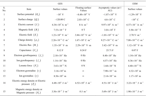
In order to get a detailed picture of the hydrodynamic GES equilibrium features, we have used the well-known fourth order Runge-Kutta method (RK-IV method) for numerical analyses of the solar plasma system. The two scale equilibrium structures of the coupled solar plasma system are governed by Equations (1)-(3) for the bounded SIP, and Equations (23)-(24) for the unbounded SWP. Two different sets of realistic initial values of the relevant solar physical variables are specified for nu-merical solutions of the basic governing equations. The first set of realistic initial values for the SIP description is analytically specified by nonlinear stability analysis, which falls within the solar core region. The values of these physical variables at the SSB are the natural out-comes of the nonlinear dynamical solutions of the SIP Equations (1)-(3) as an initial value problem. Now the numerically calculated values of these physical variables at the SSB forms the second set of realistic initial values for the SWP description as carried out in our earlier work [11]. In fact, this is the way we have solved the nonline-arly coupled governing dynamical equations of the two-layer GES model description. These two sets of re-alistic initial values are listed in Table 1 as follows.

4.1. Numerical Results for Bounded SIP

The coupled structure Equations (1)-(22) for the GES characterization are numerically simulated with the initial values as tabulated in Table 1 on the SIP scale. Figures 1-9 describe the profile structures of the SIP equilibrium in terms of the GES physical parameters. As given in Table 3 the values of i0.01,  T 0.40 and i 0.001 are kept fixed as already specified in our earlier paper [11] for all the numerical plots for the SIP scale descrip-tion. The other fixed initial values obtained by nonlinear stability analyses for the concerned characterization here are 1 2 i 0.005

si i

g  e and 1 2 2i 0.005

i i

M  e  .

Figure 1 contains the plots of the normalized solar self- gravity, its gradient and associated inhomogenity scale length (scaled down by division with 20) at various ra-dial positions from the initial location. It is clear from Figure 1 that gsdgs d 0.26 at 0.80. Near the maximum value of the solar self-gravity associated with the SIP, i.e., near the SSB, the gradient indeed be-comes zero which justifies the necessary condition for the maximization of the solar self-gravity. Moreover, near the SSB, the scale length becomes infinitely larger. The rate of spatial change of the solar self-gravity increases initially and then decreases to zero value as one approach the SSB. This means that the gravitational wall strength increases initially up to  0.80. These profiles are physically quite consistent to each others.

Figures 2(a) and 2(b) depict the plots of the GES-as-sociated normalized electrostatic potential, its gradient and associated inhomogeneity scale length. The scale length profile is non-monotonous in nature and exhibits a sudden decrease in the vicinity of the initial position and then increases rapidly. There is a minimum normalized scale length of the electrostatic potential variations of the order of 0.1. The basic features of Figure 2 near the ini-tial location can obviously be understood from Figure 2(b), which is the enlarged view of Figure 2(a). This is interestingly noted from Figure 2(b) that

d d 0.02

     at  0.54_{beyond which} increases at a faster rate (more negative value). This is found from Figures 1 and 2 that gs, dgs d and   , d d intersect approximately within the region defined by

0.54 0.80

   . This means that gs and  behave dynamically as exponentially varying functions of  as

 

s si

g  g e and  

 

_ie in this region

particu-larly, respectively. This, in turn, helps the bounded solar plasma to leak through the self-gravitational potential barrier without overflowing through it.

When the self-gravitational potential barrier height in-creases, the initial bulk flow of the SIP is drastically re-duced to the minimum possible values at the SSB as shown in Figures 3(a) and 3(b). Figures 3(a) and 3(b) depict the plots of the ion Mach number, gradient and scale length (scaled down by division with ). These plots exhibit monotonous behaviors having two scales of faster and slower regions of Mach number variations, respectively. Similarly, Figures 4(a) and 4(b) portray the plots

6

10

Table 1. Initial and boundary GES values.

Parameter At the initial location   i At the SSB    Initial values

s

g dgs d0 dgs d0, g0.60 gsi  1 2 iei

 

 ,derived

 d d  0 d d   0.62, 1.00 i, arbitrary

M dM d  e2 dM d0, _M _{~ 10}7

 Mi  1 2 iei2

 

(9)

0 0.3 0.6 0.9 1.2 1.5 1.8 2.1 2.4 2.7 3 3.3 3.5 -0.1

0 0.1 0.2 0.3 0.4 0.5 0.6 0.7 0.8 0.9 1

Normalized position

S

o

la

r

se

lf

-g

ravi

ty

, g

ra

d

ien

t an

d

s

ca

le l

e

n

g

th

Profile of SIP gravity, gradient and scale length Self-gravity

Gradient Scale length (/20)

Figure 1. Variation of the normalized values of solar self-gravity

 

gs (solid blue line), self-gravity gradient



dgs d



(red dashed line) and self-gravity scale length



 



Lg_s_1gs dgs d _



1

/20 (black dotted line) associ-ated with the SIP flow dynamics with normalized position



 



from the heliocentre



0



. The initial values 0.01

i

  ,  T 0.40 and i  0.001 are kept fixed. The

other fixed initial values by nonlinear stability analyses are

ei0.005 1 2

si i

g   and _{1 2} e2i0.005

i i

M  .

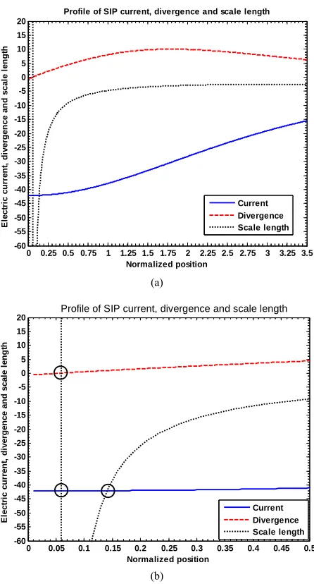
of solar plasma current density, its divergence and scale length. The gradient profile clearly shows the non-di-vergent behavior of the electron dominated current flowing through the gravitational wall of the SIP. From con-ventional viewpoint, the direction of current flow is to-wards the helio-centre. The magnitude of the current decreases as one moves from heliocentre to the SSB. The enlarged description of Figure 4(a) is given in Figure 4(b) showing the electrodynamics of the solar electric current near the heliocentre. This is found from Figure 4(b) that J_1 J



d dJ 



_142.00 at both  0.06 and  0.13. But at the position  0.06, it is seen

that d dJ   _1 J



d dJ 



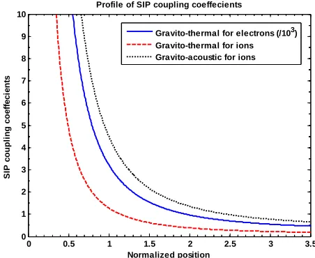
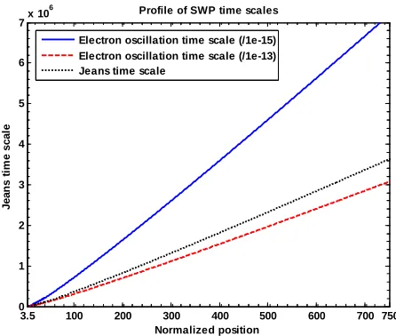
_{ }1 1.00, approximately. Figure 5 exhibits the plots of the normalized solar plasma (population) density, its gradient and scale length. Figure 6 depicts the numerical plot of the second order differential derivative of the solar self-gravity and exhib-its the validity of the condition for sufficiency of the maximization of the solar self-gravity at the SSB. Figure 7 exhibits the profiles of the normalized time scales for electron oscillations (scaled up by division with ₁₀15_),

SIP ion oscillation (scaled up by division with ₁₀13₎

and Jeans collapse. It is clear to note that the Jeans time scale is quite larger by several orders of magnitude rela-tive to each of the rest. Figure 8 depicts the plots of the normalized coupling constants for the gravito-thermal

0 0.3 0.6 0.9 1.2 1.5 1.8 2.1 2.4 2.7 3 3.3 3.5 -1.4

-1.2 -1 -0.8 -0.6 -0.4 -0.2 0 0.2 0.4 0.6 0.8 1 1.2 1.4 1.6 1.8 2 2.2 2.4 2.6

E

lectro

st

ati

c

p

o

ten

ti

al

, g

rad

ie

n

t

an

d

scal

e l

e

n

g

th

Profile of SIP electrostatic potential, gradient and scale length Electrostatic potential

Gradient Scale length

(a)

0 0.1 0.2 0.3 0.4 0.5 0.6 0.7 0.8 0.9 1 -0.2

-0.15 -0.1 -0.05 0 0.05 0.1 0.15 0.2 0.25 0.3 0.35 0.4

E

lect

ro

st

a

ti

c

p

o

te

n

ti

al

, g

rad

ien

t an

d

scal

e l

e

n

g

th

Profile of SIP electrostatic potential, gradient and scale length

Electrostatic potential Gradient

Scale length

(b)

Figure 2. (a) Variation of the normalized values of electro-static potential

 

 (solid blue line), potential gradient



d d 



(red dashed line) and potential scale length







_ d d _1

 

1

L_   (black dotted line) associated with the SIP flow dynamics with normalized position



 





0



under the same initial condi-tions as in Figure 1; (b) Same as Figure 2(a), but in a magnified form.

coupling for the SIP electrons, gravito-thermal coupling for the SIP ions and gravito-acoustic coupling for the SIP ions.

(10)

0 0.3 0.6 0.9 1.2 1.5 1.8 2.1 2.4 2.7 3 3.3 3.5

-10 -9 -8 -7 -6 -5 -4 -3 -2 -1 0 1 2 3 4 5x 10

-6 Normalized position M a c h n u m b e r, g rad ie n t an d sc al e l e n g th

Profile of SIP Mach number, gradient and scale length Mach number Gradient Scale length (/106)

(a)

0 0.25 0.5 0.75 1 1.25 1.5 1.75 2 2.25 2.5 2.75 3 3.25 3.5 -10 -9 -8 -7 -6 -5 -4 -3 -2 -1 0 1 2 3 4 5x 10

-7 Normalized position M ach n u m b er , g rad ien t an d sca le l en g th

Profile of SIP Mach number, gradient and scale length

Mach number Gradient Scale length (/106)

(b)

Figure 3. (a) Variation of the normalized values of Mach number

 

M (solid blue line), Mach number gradient



dM d



(red dashed line) and Mach number scale length







_ d d _1 ₆



1 10

LM M M   (black dotted line) associated with the SIP flow dynamics with normalized position



 





0



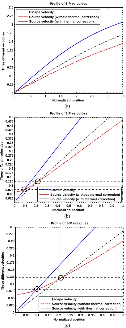
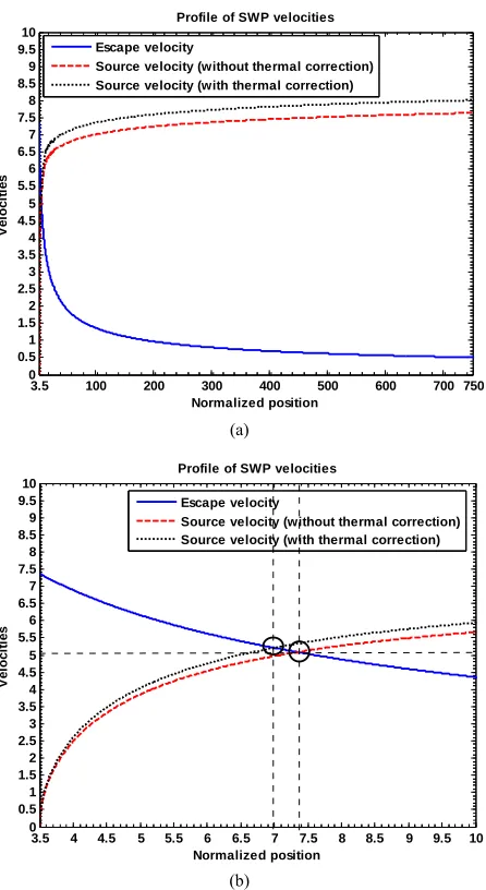
under the same initial conditions as in Figure 1; (b) Same as Figure 3(a) but in a magnified form.

the heliocentre, respectively. This is now observed that at

0.08 s

v_ v   0.1 and v_sv_st0.125 at

0.21

  showing the intersecting dynamics near the heliocentre. This is to note that the bulk SIP leaks through the self-gravitational wall by plasma-boundary interaction and finally emerges out in the form of the subsonic SWP at the SSB due to gravitational squeezing of the electron flux as discussed earlier.

0 0.25 0.5 0.75 1 1.25 1.5 1.75 2 2.25 2.5 2.75 3 3.25 3.5 -60 -55 -50 -45 -40 -35 -30 -25 -20 -15 -10 -5 0 5 10 15 20 Normalized position E lect ri c cu rr en t, d ive rg e n ce a n d sc al e l en g th

Profile of SIP current, divergence and scale length

Current Divergence Scale length

(a)

0 0.05 0.1 0.15 0.2 0.25 0.3 0.35 0.4 0.45 0.5

-60 -55 -50 -45 -40 -35 -30 -25 -20 -15 -10 -5 0 5 10 15 20 Normalized position E lect ri c cu rr en t, d iver g en ce an d sca le l en g th

Profile of SIP current, gradient and scale length

Current Divergence Scale length

Profile of SIP current, divergence and scale length

(b)

Figure 4. (a) Variation of the normalized values of electric current density

 

J (solid blue line), divergence of cur-rent density



d dJ 



(red dashed line) and current den-sity scale length



LJ_1J



d dJ 



_1



(black dotted line) associated with the SIP flow dynamics with normalized position



 





0



under the same initial conditions as in Figure 1; (b) Same as Figure 4(a), but in a magnified form.

4.2. Numerical Results for Unbounded SWP

Similar to the bounded SIP analyses, here too, we simu-late the coupled dynamical evolution Equations (23)-(35) on the SWP scale with the numerically pre-obtained ini-tial values as shown in Table 1. Figures 10-16 describe the profile structures of the SWP equilibrium in terms of the proposed GES plasma parameters. The predeter-mined values of the physical variables for the SSB, viz.,

3.5 SSB

  ,  T 0.1, ,

7 10 SSB

[image:10.595.56.285.72.504.2] [image:10.595.312.535.74.488.2]

(11)

0 0.5 1 1.5 2 2.5 3 3.5 -0.5

-0.25 0 0.25 0.5 0.75 1

P

opul

a

ti

on de

ns

it

y

, gr

a

di

e

nt

a

nd

s

c

a

le

l

e

ngt

h

[image:11.595.60.286.78.259.2]

Profile of SIP density, gradient and scale length Density Gradient Scale length (/102)

Figure 5. Variation of the normalized values of population density

 

e (solid blue line), density gradient



ed d 



(red dashed line) and density scale length



ed d 







 



d d 2

/10

 

n

L 



(black dotted line) associated with

the SIP flow dynamics with normalized position



 





0



under the same initial condi-tions as in Figure 1.

0.5 1 1.5 2 2.5 3 3.5 4

0.1 -5 -4 -3 -2 -1 0 1 2 3 4 5x 10

-5

S

ec

o

n

d

er

ivat

ive o

f se

lf

-g

ra

vi

ty

[image:11.595.310.536.80.267.2]

Profile of SIP self-gravity curvature

Figure 6. Variation of the normalized value of the second derivative of self-gravity



d2 d 2



s

g  (solid black line) associated with the SIP flow dynamics with normalized position



 





under the same initial conditions as in Figure 1.



0



2

0 s J 95

a GM_ c   are kept fixed throughout. Fig- ures 10(a) and 10(b) depict the equilibrium profiles of the normalized electrostatic potential, its gradient (scaled up by multiplication with 10) and scale length (scaled down by division with ) associated with the GES on the SWP scale. Figure 10(b) shows the same plot as shown in Figure10(b), but in a magnified form.

2

10

0 0.5 1 1.5 2 2.5 3 3.5

0.5 1 1.5 2 2.5 3 3.5

T

im

e scal

es

[image:11.595.61.285.362.552.2]

Profile of SIP time scales Electron oscillation time scale (/1e-15) Ion oscillation time scale (/1e-13) Jeans Time scale

Figure 7. Variation of the normalized values of (a) electron oscillation time scale



15



/10

pe

 

(blue solid line), (b) ion oscillation time scale



13



/10

pi

 

(red dashed line) and (c) Jeans time scale

 

J (black dotted line) associated with

the SIP flow dynamics with normalized position



 





0



under the same initial condi-tions as in Figure 1.

0 0.5 1 1.5 2 2.5 3 3.5

0 1 2 3 4 5 6 7 8 9 10

S

IP

c

oup

li

ng c

oe

ff

e

c

ie

n

ts

Profile of SIP coupling coeffecients

Gravito-thermal for electrons (/103) Gravito-thermal for ions Gravito-acoustic for ions

Figure 8. Variation of the normalized values gravitothermal coupling coefficient for electrons



 

3



/10

e

 (blue solid

line), gravito-thermal coupling coefficient for ions (i) (red

dashed line) and gravito-acoustic coupling coefficient for ions

 

a (black dotted line) associated with the SIP flow

dynamics with normalized position



 



from the heliocentre



0



under the same initial conditions as in Figure 1.

[image:11.595.309.535.371.556.2]

(12)

0 0.5 1 1.5 2 2.5 3 3.5 0 0.25 0.5 0.75 1 1.25 1.5 1.75 2 2.25 2.5 Normalized position Thr e e di ff e re n t v e lo c it ie s

Profile of SIP velocities

Escape velocity

Source velocity (without thermal correction) Source velocity (with thermal correction)

(a)

0 0.1 0.2 0.3 0.4 0.5 0.6 0.7 0.8 0.9 1 0 0.025 0.05 0.075 0.1 0.125 0.15 0.175 0.2 0.225 0.25 0.275 0.3 0.325 0.35 0.375 0.4 0.425 0.45 0.475 0.5 Normalized position Th re e di ff e re nt v e loc it ie s

Escape velocity

(b)

0 0.05 0.1 0.15 0.2 0.25 0.3 0.35 0.4 0.45 0.5 0 0.025 0.05 0.075 0.1 0.125 0.15 0.175 0.2 0.225 0.25 0.275 0.3 Normalized position Thr e e di ff e re nt v e loc it ie s

Escape velocity

(c)

Figure 9. (a) Variation of the normalized values of escape velocity of ions (blue solid line), source velocity without thermal correction of ions (red dashed line) and source velocity with thermal correction of ions

 

v

 

vs

 

vst

(black dotted line) associated with the SIP flow dynamics with normalized position



 



under the same initial conditions as in Figure 1; (b) Same as Figure 9(b), but in a magnified form; (c) Same as Figure 9(a), but in a more magnified form.



0

100 200 300 400 500 600 700

3.5 750 -40 -30 -20 -10 0 10 20 30 40 50 60 70 80 90 100 110 120 Normalized position E lect ro s tat ic p o ten ti al , g rad ien t an d sca le l en g th

Profile of SWP electrostatic potential, gradient and scale length Electrostatic potential

Gradient (X101) Scale length (/102)

(a)

3.5 4 4.5 5 5.5 6 6.5 7 7.5 8 8.5 9 9.5 10 10.5 11 11.5 12 12.5 -20 -17.5 -15 -12.5 -10 -7.5 -5 -2.5 0 2.5 5 7.5 10 12.5 15 Normalized position E le ct ro st at ic p o ten ti al , g rad ie n t a n d scal e l en g th

Profile of SWP electrostatic potential, gradient and scale length Electrostatic potential Gradient (X101) Scale length (/102)

(b)

Figure 10. (a) Variation of the normalized values of electro- static potential

 

 (solid blue line), potential gradient







d d  10



(red dashed line) and potential scale length







_{ } d d _ 2

1 / 10

L_    1 (black dotted line) associated with the SWP flow dynamics with normalized position



 



from the SSB



3.5



3.5

SSB

. The predetermined SSB

parameter values   ,  _T 0.1 ,  7

10

SSB

 

, 1

  , and a0 G 2s J are kept fixed; (b)

Same as Figure 10(a), but in a magnified form. 95



M c 



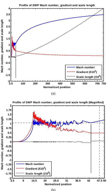
that in the entire sonic zone, dM d decreases with 

ymptotically. This can be justified by the binomial simplification of the L.H.S. of Equation (24) near the singular sonic point as defined by

as

M  . Under the

condition



M 







1a0 2



, we reduce

equa-tion (24) to



dM d



 . This immediately implies that the supersonic/ hypersonic unbounded SWP outflow is the outcome of the curvature (geometrical) effect of the spherically bounded subsonic SIP mass distribution. Figure 11(b) shows the same plot as shown in Figure

[image:12.595.63.267.76.608.2] [image:12.595.311.532.79.474.2]

(13)

100 200 300 400 500 600 700 3.5 750 -2 -1.5 -1 -0.5 0 0.5 1 1.5 2 2.5 3 3.5 4 Normalized position M ach n u m b er, g rad ie n t an d scal e l en g th

Profile of SWP Mach number, gradient and scale length

Mach number Gradient (X101) Scale length (/103)

(a)

3.5 9 14.5 20 25.5 31 36.5 42 47.5 50

-2 -1.75 -1.5 -1.25 -1 -0.75 -0.5 -0.25 0 0.25 0.5 0.75 1 1.25 1.5 1.75 2 Normalized position M ach n u m b er , g ra d ien t an d sc al e l en g th

Profile of SWP Mach number, gradient and scale length (Magnified)

Mach number Gradient (X101) Scale length (/103)

(b)

Figure 11. (a) Variation of the normalized values of Mach number

 

M (solid blue line), Mach number gradient







10



dM d



(red dashed line) and Mach number scale

length



_M 









d d 

1 1/ 103

L M M  



(black dotted line) associated with the SWP flow dynamics with normalized position   from the SSB under the same initial conditions as in Figure 10(a); (b) Same as Figure 11(a), but in a magnified form.



3.5



11(a), but in a magnified form depicting the vivid picture of the sonic zone associated and followed with the onset of the supersonic/ hypersonic SWP flow dynamics.

Figures 12(a)-12(c) describe the profile structure of the normalized SWP current, divergence (scaled down by division with ) and scale length (scaled down by division with ). Figure12(b) shows the same plot as shown in Figure 12(a), but in a magnified form. Fur-thermore, Figure12(c) depicts the same plot as shown in Figure 12(a), but in a more magnified form describe-

3

10

2

10

100 200 300 400 500 600 700

3.5 750 -10 -7.5 -5 -2.5 0 2.5 5 7.5 10 Normalized position E lect ri c c u rr e n t, d iv er g en ce a n d sc al e l en g th

Profile of SWP current, divergence and scale length

Current Divergence (/103₎

Scale length (/102₎

(a)

3.5 9 14.5 20 25.5 31 36.5 42 47.5 50 -10 -7.5 -5 -2.5 0 2.5 5 7.5 10 Normalized position E lectr ic cu rr en t, d iver g en ce an d scal e l en g th

Profile of SWP current, divergence and scale length (Magnified)

Current Divergence (/103₎

Scale length (/102₎

(b)

3.5 4 4.5 5 5.5 6 6.5 7 7.5 8 8.5 9 9.5 10 10.5 11 11.5 12 12.5 -10 -7.5 -5 -2.5 0 2.5 5 7.5 10 Normalized position E le c tr ic c u rr e n t, d ive rg en ce an d s cal e l e n g th