Essays on multi asset jump diffusion models : estimation, asset allocation and American option pricing

(1)

warwick.ac.uk/lib-publications

A Thesis Submitted for the Degree of PhD at the University of Warwick

Permanent WRAP URL:

http://wrap.warwick.ac.uk/93986

Copyright and reuse:

This thesis is made available online and is protected by original copyright. Please scroll down to view the document itself.

Please refer to the repository record for this item for information to help you to cite it. Our policy information is available from the repository home page.

(2)

(3)

List of Figures

2.1 Correlation between arithmetic and geometric averages . . . 15

2.2 Comparison of convergence speeds of MLSM and OLSM for pric-ing American arithmetic average option on 6 assets . . . 26

2.3 Effects of volatility, time-to-maturity and strike price on pricing error. All stocks have the same setting as Example 2.3, i.e., Common Initial Price Si0 = 100, Strike Price K=100, Interest rate r=3%, no Dividend, Maturity T=1 Year, Common Volatility σi1 = 20%, Common Correlation ρij = 0.5, i 6= j = 1, ...,10,

if not otherwise mentioned. In particular, the pricing error is calculated with SPSA estimators as benchmark and M=10000. . 29

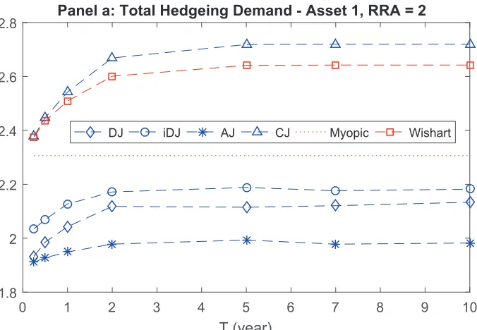
3.1 Total Hedging Demand against Time Horizon against various models . . . 65

3.2 Hedging Demand against C2(1) (DJ) . . . 66

3.3 Hedging Demand against C1(1) (DJ) . . . 66

3.4 Hedging Demand of Asset 1 against J21 J12 (DJ) . . . 67

3.5 Hedging Demand of Asset 2 against J21 J12 (DJ) . . . 68

4.1 Illustration of Single-variate Slice Sampling Method . . . 103

4.2 Illustration of Metropolis-Hasting and slice sampling scheme . . 104

4.3 Fitted Variance-Covariance states - Σt11 . . . 115

4.6 Asymmetric Correlation - Market and Consumer portfolios . . . 119

4.7 Asymmetric Correlation - Market and Manufacturing portfolios 120 4.8 Asymmetric Correlation - Market and High-Technology portfolios 120 4.9 Asymmetric Correlation - Market and Health portfolios . . . 120

(6)

List of Tables

2.1 American Arithmetic Average Options on 1 to 6 underlying stocks. 30 2.2 American Arithmetic Average Option on 10, 30 and 50

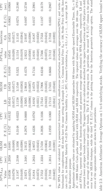
underly-ing stocks followunderly-ing MJD process. . . 31 2.3 American Arithmetic Average Options on 1 to 6 underlying stocks.

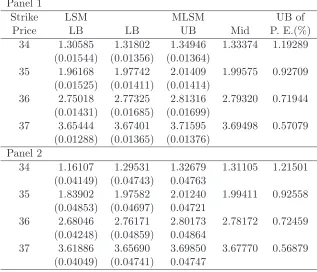
Verifying the accuracy of MLSM upper bound with SPSA approach. 32 2.4 American Arithmetic Average Option on 30 assets with 20 long

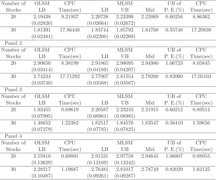
positions and 10 short positions. . . 33 2.5 American Arithmetic Average Option on 20 and 30 underlying

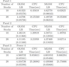
stocks with different volatilities. . . 34 2.6 American Arithmetic Average Option on 10 and 20 assets with

Heston’s model of stochastic volatility. . . 35 2.7 American Arithmetic Average Options on 10 underlying stocks. 36 3.1 Optimal Hedging Demands for 2 Risky Assets with Two Jumps

Entangled . . . 70 3.2 Optimal Hedging Demands for 2 Risky Assets with Two Jumps

Entangled . . . 73 3.5 Optimal Hedging Demands for 2 Risky Assets with Two

Inde-pendent Jumps . . . 74 3.6 Optimal Hedging Demands for 2 Risky Assets with Two

(7)

3.9 Optimal Variance Hedging Demands for 2 Risky Assets with

Jumps in Returns Only . . . 78

3.10 Optimal Covariance Hedging Demands for 2 Risky Assets with Jumps in Returns Only . . . 79

3.11 Optimal Asset Jump Hedging Demands for 2 Risky Assets with Jumps in Returns Only . . . 80

3.12 Optimal Variance Hedging Demands for 2 Risky Assets with Jumps in Covariance Matrix Only . . . 81

3.13 Optimal Covariance Hedging Demands for 2 Risky Assets with Jumps in Covariance Matrix Only . . . 82

3.14 Parameters adopted for numerical experiments. . . 83

4.1 Simulation tests for entangled MJD model, T=1000 . . . 109

4.2 Simulation tests for entangled MJD model, T=3000 . . . 110

4.3 Simulation tests for 1 dimensional stochastic volatility model. . 111

4.4 Simulation tests for WJD-DJ model with 500 simulated time series112 4.5 Simulation tests for WJD-DJ model with 1000 simulated time series . . . 113

4.6 Simulation tests for WJD-DJ model with 2000 simulated time series . . . 114

(8)

(9)

Acknowledgement

There has been so many people who directly or indirectly help during my Ph.D studies. Firstly, I have to deliver my sincerest gratefulness to my supervisor, Dr. Xing Jin, who not only guides my Ph.D studies, but also shares his philosophy of life. During this long lasting Ph.D life, I have learned a lot from him and without his guidance, I would have wasted more times struggling for finding the right way to make myself prepared for academic research. Moreover, when I felt depressed and stressed, his encouragement, enthusiasm and support always revive me from those negative sentiments. I would also like to thank my second supervisor, Dr. Sarah Qian Wang also shares her experience in preparing for job markets and ways of doing research. Although we have no collaboration work yet, I can still feel her patience and kindness for guiding me.

Apart from my supervisors, I would like to express my heartfelt appreciation to the entire Finance group at Wariwck Business School, where kindly and in-sightful comments and frequent interactions often provide me new ideas and broaden my mind. In particular, I would especially thank Andrea Gamma and Michael Moore for organizing special events.

Besides, I also appreciate my close friends, including Yao Chen, Linquan Chen and Chunling Xia, Jeff Hung, Harold Contreras Munoz, and many others, made during these years. They are not only colleagues whom I spent those sleepless night with but also friends to share lives with. Without their company, I would not experience a Ph.D life as wonderful as it has been.

(10)

Declaration

I declare that the three essays included in this thesis has not been submitted for a degree to any other university. Moreover, Chapter 2 and Chapter 4 are collaboration works with my supervisor, Dr. Xing Jin, while Chapter 3 is a col-laboration work with Dr. Xing Jin and Dr. Xudong Zeng (School of Finance, Shanghai University of Finance and Economics).

(11)

Abstract

In the first essay(Chapter 2), we develop an efficient payoff function approxi-mation approach to estimating lower and upper bounds for pricing American arithmetic average options with a large number of underlying assets. This method is particularly efficient for asset prices modeled by jump-diffusion pro-cesses with deterministic volatilities because the geometric mean is always a one-dimensional Markov process regardless of the number of underlying assets and thus is free from the curse of dimensionality. Another appealing feature of our method is that it provides an extremely efficient way to obtain tight upper bounds with no nested simulation involved as opposed to some existing duality approaches. Various numerical examples with up to 50 underlying stocks sug-gest that our algorithm is able to produce computationally efficient results.

Chapter 3 solves portfolio choice problem in multi-dimensional jump-diffusion models designed to capture empirical features of stock prices and financial con-tagion effect. To obtain closed-form solution, we develop a novel general decom-position technique with which we reduce the problem into two relative simple ones: Portfolio choice in a pure-diffusion market and in a jump-diffusion mar-ket with less dimension. The latter can be reduced further to be a bunch of portfolio choice problems in one-dimensional jump-diffusion markets. By virtue of the decomposition, we obtain a semi-closed form solution for the primary optimal portfolio choice problem. Our solution provides new insights into the structure of an optimal portfolio when jumps are present in asset prices and/or their variance-covariance.

(12)

Abbreviation

AA: Arithmetic average GA: Geometric average

OLSM: Ordinary least square Monte Carlo MLSM: Modified lease square Monte Carlo MCMC: Markov Chain Monte Carlo MH: Metropolis-Hasting

WJD: Wishart-Jump-Diffusion (model) DJ: Double jump (model) iDJ: Independent double jump (model)

AJ: asset jump (model) CJ: covariance jump (model)

MJD: Merton-Jump-Diffusion (model) SV: Stochastic volatility (model)

SVMJ: Stochastic volatility with Merton Jump (model)

SVCMJ: Stochastic volatility with common Merton Jump (model) SDE, ODE: stochastic/ordinary differential equations

HJB: Hamilton-Jacobi-Bellman (equation) ML: Maximum Likelihood (method) QML: Quasi-Maximum Likelihood (method)

SML: Simulated Maximum Likelihood (method) GMM: Generalized Method of Moment (method) EMM: Efficient Method of Moment (method)

(13)

Chapter 1 General Introduction

In this thesis, I aim to provide insightful researches that help investors to op-timally manage their wealth, which may be one of the original motivation of finance studies. With the growing innovation in technology and increasingly en-tangled financial markets, every investor is exposed to all sources of economic risks domestically, or internationally. The first idea that comes into my mind is finding a good hedging vehicle for a portfolio.

In Chapter 2, we develop an efficient payoff function approximation approach to estimating lower and upper bounds for pricing American arithmetic aver-age options with a large number of underlying assets. The crucial step in the approach is to find a geometric mean which is more tractable than and highly correlated with a given arithmetic mean. Then the optimal exercise strategy for the resultant American geometric average option is used to obtain a low-biased estimator for the corresponding American arithmetic average (AA) option. This method is particularly efficient for asset prices modeled by jump-diffusion pro-cesses with deterministic volatilities because the geometric mean is always a one-dimensional Markov process regardless of the number of underlying assets and thus is free from the curse of dimensionality. Another appealing feature of our method is that it provides an extremely efficient way to obtain tight upper bounds with no nested simulation involved as opposed to some existing dual-ity approaches. Various numerical examples with up to 50 underlying stocks suggest that our algorithm is able to produce computationally efficient results. With such efficient American AA pricing tool, it is feasible to hedge a large portfolio with the corresponding American AA option.

(14)

react during financial crisis would be of great research value since it helps for preventing investors from portfolio loss. Recent empirical studies find stock prices tend to have big move together and a big jump may be followed by more frequent jumps, which is especially evident during financial crisis.

In Chapter 3, We study the portfolio choice problem in multi-dimensional jump-diffusion models designed to capture these empirical features and capture the financial contagion effects. To obtain closed-form solution, we develop a novel general decomposition technique with which we reduce the problem into two relative simple ones: Portfolio choice in a pure-diffusion market and in a jump-diffusion market with less dimension. The latter can be reduced further to be a bunch of portfolio choice problems in one-dimensional jump-diffusion mar-kets. By virtue of the decomposition, we obtain a semi-closed form solution for the primary optimal portfolio choice problem. Our solution provides new insights into the structure of an optimal portfolio when jumps are present in asset prices and/or their variance-covariance. Our results show that the jumps in the variance-covariance have important effects on the asset allocations, espe-cially when there are jumps in the asset prices simultaneously. Meanwhile, the hedging demands for jumps are much more significant compared to variance or covariance hedging demands for diffusion risks and ignoring jump risk in the variance-covariance may cause large wealth equivalent loss in the presence of jumps in the asset prices. In addition, two novel components integrated to cap-ture empirical feacap-tures are verified to cause significant effects in the resulting optimal portfolio wrights. As a result, the proposed multivariate model provides an potential ideal model to study financial contagion. Moreover, with optimal portfolio problem solved with semi-closed form solution, financial contagion may be studied in the context of asset allocation quantitatively. To some extent, this paper sheds new lights on the financial contagion and portfolio choice literatures.

(15)

e.g. stochastic volatility model with common jump in Eraker et al. (2003), among others.

(16)

Chapter 2 Efficient estimation of lower and

upper bounds for pricing

higher-dimensional American

arithmetic average options by

approximating their payoff

functions

1

2.1 Introduction

The importance of American-style options has been growing increasingly and pricing of American options especially high-dimensional cases remains one of the challenging problems both theoretically and practically in the option pric-ing theory. In particular, high-dimensional American options would be valuable research topics. For example, Shiu et al (2013) document that basket warrants, essentially basket options with multiple underlying assets become more popular over the past decade.2 _{In this paper, we focus on pricing American arithmetic}

average options. The appealing advantage of an American arithmetic average option lies in the fact that it exactly replicates the evolution of the portfolio

1

This paper has been published on International Review of Financial Analysis 44 (2016):

65-77

2

(17)

formed by the underlying assets. For example, the cost of hedging a portfo-lio with an American arithmetic average option is much lower than a portfoportfo-lio of individual options on the same underlying assets since the former takes the correlations among the underlying assets into account and only one option is involved in hedging. Besides, it would be simple for investors to replicate the payoff of any portfolio without actually holding the portfolio if there is such an American arithmetic average option available on the market. Given these significant applications, efficient pricing methods for American arithmetic av-erage options written on the avav-erage of multiple underlying assets are of great value from various points of view such as hedging and risk management espe-cially after the recent financial crisis that re-emphasized the importance of risk management. The purpose of this paper is to develop an efficient approach to obtaining lower and upper bounds for American arithmetic average option prices on a large number of underlying assets.

The traditional valuation methods, such as lattice and tree-based techniques, for pricing high dimensional American option pricing problems are typically plagued by the curse of dimensionality and thus, simulation-based numerical methods are inevitably required. Earlier literature about simulation-based ap-proaches can be traced back to Boyle (1977) in which European style claim is priced with Monte Carlo (MC) simulation. American style option pricing tech-niques with MC simulation include Bundling Methods in Tilley (1993), Strati-fied State Aggregation (SSA) in Barraquand and Martineau (1995), Stochastic Mesh Method (SMM) in Broadie and Glasserman (2004), regression-based ap-proach in Tsitsiklis and Van Roy (1999) and Longstaff and Schwartz (2001), among others.

The existing simulation-based methods can be categorized into: (1) Primal approach, which aims to obtain a lower bound for an American option by esti-mating a suboptimal exercise strategy, e.g., regression-based approaches as in Tsitsiklis and Van Roy (1999) and Longstaff and Schwartz (2001); (2) Duality approach, which estimates an upper bound for an American option by using a dual martingale, e.g. Rogers (2002), Haugh and Kogan (2004) and Anderson and Broadie (2004).

(18)

has been well established in Carriere (1996), Tsitsiklis and Van Roy (1999) and Longstaff and Schwartz (2001), etc. Related convergence analysis and simula-tion issues can be found in Tsitsiklis and Van Roy (2001), Cl´ement et al. (2002), Glasserman and Yu (2004a,b) and Stentoft (2004).

In particular, the least squares method (LSM) developed by Longstaff and Schwartz (2001) is the most widely used method due to its simplicity and gener-ality. A lower bound of an American option can be obtained from a suboptimal optimal exercise strategy derived from linear regression procedure. However, this method and other primal approaches are becoming computationally expen-sive with the increasing dimension of pricing problem and hence the trade-off between computational costs and efficiency of approximation would be a critical issue.

A variety of methods have been proposed to improve the performance of regression-based approaches. For instance, to address arbitrary style of continuation val-ues, Kohler et al (2010) use least square neural network regression estimates and estimate continuation values from artificial MC simulated paths. Their approach is more general than LSM since the regression is nonparametric. But, compared to LSM, the nonparametric in Kohler et al (2010) would be even worse to implement for pricing high-dimensional American options.3 _{More recently,}

Jain and Oosterlee (2012) proposed a stochastic grid method (SGM) which could be regarded as a hybrid of Barraquand and Martineau (1995): stratified sampling along pay-off method, Longstaff and Schwartz (2001): Least square Monte Carlo method and Broadie and Glasserman (1997b): stochastic mesh method. The proposed SGM algorithm is more suitable for pricing some high-dimensional American options than existing methods. However, SGM would be computationally costly when sub-simulations are embedded and more early exercise times are allowed.

To circumvent the curse of the dimensionality problem associated with pricing of multi-dimensional American options, several dimension reduction methods have been proposed. For example, Barraquand and Martineau (1995) introduce a partitioning algorithm. Their method differs from Tilley’s bundling algorithm in that they partition the payoff space instead of the state space. Hence, only a one-dimensional space is partitioned at each time step, regardless the dimen-sion of the problem. More recently, Jin et al (2013) further integrate this idea

3

(19)

into state-space partitioning algorithm (SSPM) developed by Jin, Tan and Sun (2007) and improve the computational efficiency significantly with computa-tional accuracy preserved. Those papers, however, do not provide an algorithm for upper bounds.

In the present paper, we follow the dimension reduction approach to pricing high-dimensional American arithmetic average options. The key idea is to find a highly correlated geometric average for a given arithmetic average. As will become clear later, the former is more tractable than the latter in the sense that the geometric average has a lower dimension4 _{than the corresponding arithmetic}

average, and thus the optimal exercise strategy for the American geometric av-erage option is far easier to obtain than for the American arithmetic avav-erage option. In particular, when the asset prices are modeled by jump-diffusion processes with deterministic volatilities, the geometric mean is always a one-dimensional Markov process regardless of the number of underlying assets, and thus is free from the curse of dimensionality. Then the optimal exercise strategy for the American geometric average option is used to obtain a lower bound for the corresponding American arithmetic average option. In addition, by using an inequality similar to (4) in Haugh and Kogan (2004), we provide an extremely fast way to obtain the corresponding upper bound without nested MC simula-tions. To be more specific, in the inequality (4) in Haugh and Kogan (2004), we approximate the payoff function of given American arithmetic average option by the one of a highly correlated American geometric average option. Unlike Haugh and Kogan (2004), we do not need to find the optimal supermartingale and thus we do not need nested MC simulations.

An important limitation of the lower bound is that it is not easy to evalu-ate the accuracy of its approximation to the true option price. Upper bounds in combination with the corresponding lower bounds allow us to measure the accuracy of price estimators for American average options. In earlier litera-ture, Broadie and Glasserman (1997, 2004) propose stochastic mesh methods which generate not only lower but also upper bounds and both bounds converge

4

(20)

asymptotically to the true value. Despite the advantage of obtaining the up-per bound, the stochastic mesh methods are quite computationally demanding. Boyle et al (2003) further generalizes Broadie and Glasserman (1997, 2004) with a low-discrepancy sequence for efficiency.

Independently developed by Rogers (2002), Anderson and Broadie (2004) and Hough and Kogan (2004), duality approach is the most general technique among those upper bound related approach. The idea is to introduce a dual martingale in the pricing problem and rewrite the primal problem into a dual minimization problem. For example, Anderson and Broadie (2004) use nested MC simulation to approximate the optimal exercise strategy. On the other hand, Hough and Kogan (2004) apply an intensive neural network algorithm and low discrepancy sequences to estimate the option prices. However, their estimation techniques to estimate dual martingale do not preserve the martingale property in general and the computational cost is generally high.

To improve this, Glasserman and Yu (2004b) proposed a special regression algorithm to preserve the martingale property. Nonetheless, the martingale property Condition (C3) on the basis functions may not be straightforward to verify in practice. In terms of efficiency, Kolodko and Schoenmakers (2004) try to overcome the computational inefficiency of nested simulation by choosing a different estimator to reduce the number of inner path simulations. However, the upper bound is not guaranteed by their estimator as the number of inner path is too few.

(21)

In summary, we have made two contributions to the literature of pricing high-dimensional American arithmetic average options. First, we have developed a computationally efficient dimension reduction method to estimate lower bound. Second, we provide an easy-to-implement approach to evaluate the upper bound which involves no nested simulation and is based on a simple linear regression procedure. We are not aware of any research in the current literature that estimates lower and/or upper bounds for pricing high-dimensional American arithmetic average options via geometric mean approximation. As mentioned above, the essence of our algorithm is to approximate an arithmetic average by a lower-dimensional and more tractable geometric average which is highly correlated with the arithmetic average. In contrast, extant literature usually approximates the continuation values of American options.

The remaining of this paper is organized as follows. In Section 2, we introduce basic dynamic programming framework for pricing American-style options. In Section 3, we provide some theoretical considerations and empirical tests that justify using a highly correlated geometric mean to approximate a given arith-metic mean. Then we present procedures for estimating lower and upper bounds for pricing American arithmetic average options. In Section 4, various numer-ical experiments are provided to illustrate the performance of our algorithms. Section 5 concludes the paper.

2.2 The model and valuation

In this section, we first introduce American arithmetic average options and then formulate the American option pricing framework by using dynamic program-ming approach.

2.2.1 The model

Following the literature, we consider a Bermudan-style arithmetic average op-tion with n underlying stocks and strike price, K. The option is exercisable at any date in the set Γ =_{t0 = 0, t1, ..., tN =T}whereT is the pre-specified

(22)

t_∈Γ of an American arithmetic average option is defined as

hA_t(St) = K −

n

X

i=1

aiSit

!+

, (2.1)

whereSt= (S1t, ..., Snt),Sitdenotes the price of theith underlying asset at time

t,i= 1, ..., nandai represents the weight of theith stock satisfying conditions: ai >0, i= 1, ..., nandPn_i₌₁ai = 1. It is straightforward to define a call option.

It is worth mentioning that the two restrictions above can be readily relaxed. For example, a short position can be allowed in the ith stock, i.e., ai <0. For simplicity, assume that ai > 0, i = 1, ..., n0 and ai < 0, i = n0 + 1, ..., n with

n0 ≤n. In this case, the sum in (2.1) can be expressed as

n

X

i=1

aiSit = n0

X

i=1

aiSit₋ n

X

i=n0+1

(₋ai)Sit

As shown later, the sum Pn_i₌₁aiSit can be approximated by the difference of two geometric means and thus, the dimension of the pricing problem is reduced.

2.2.2 Pricing American options by dynamic

program-ming algorithm

In this section, we formally illustrate the dynamic programming formulation for pricing American options. To this end, consider an economy described by the probability space (Ω, F, P) where Ω is the sample space, F is the σ-algebra and P is a risk-neutral probability measure. Following the literature, we formulate a general class of American option pricing problem through an Rd_{-valued Markov process}_X ₌_{_Xt,₀_≤_t_≤_T_}_(with_X

0 fixed) defined on the

probability space, where the American option can be exercised at any timeτ on or before the pre-specified maturity T. The process X represent the prices of underlying assets, volatilities, interest rates and other state variables.5_{At each}

time, ti, i = 0, ..., N, the option buyer makes the exercising decision based on the dynamic programming framework. More specifically, given a nonnegative adapted payoff function,hti, the buyer chooses to exercise the option and gains

hti if the payoff is greater than the continuation value at time ti. Let Γi denote

5

For notational simplicity,Stor S is adopted hereafter since we focus on the stock price as the

(23)

the set of stopping times (with respect to the history of S) taking values in

{ti, ..., tN =T}. The option value at time ti can be defined as:

Vti(x) = sup

τ∈Γi

Ethe−

Rτ

tir(s)ds_hτ

Sti =x

i

, x∈Rd

for i = 0, ..., N, where {r(t),0 ≤ t ≤ T} is the the instantaneous short rate process.

As a result, the option value at time 0 is determined by the dynamic pro-gramming algorithm:

VtN(x) = htN(x)

Vti(x) = max

n

hti(x), Et

h

e−Rtiti+1r(s)ds_Vt

i+1(Sti+1)

Sti =x

io

, i= 0, ..., N −1.

Conventionally, we define the continuation value as

Cti(x) = Et

h

e−Rtiti+1r(s)ds_Vt

i+1(Sti+1)

Sti =x

i

, x∈Rn, i= 0, ..., N −1.

Then the option value at ti satisfies

Vti(x) = max{hti(x), Cti(x)}, i= 0, ..., N −1.

2.3 Lower and upper bounds

In this section, we propose simulation-based approaches to estimating lower and upper bounds for pricing American arithmetic average options. The key step, as aforementioned, is to construct a highly correlated geometric average for a given arithmetic average. In the next subsection, we first illustrate the construction of the correlated geometric average and then investigate both theoretically and empirically the correlation between the two variables to justify our approaches.

2.3.1 Arithmetic mean and geometric mean

(24)

the price dynamics of theith stock is as follows:

dSit

Sit = (r−qi−σi2λk)dt+σi1dWit+σi2

"

eJ ₋₁_dN

t, i= 1, ..., n,

wherer is a constant risk free rate, qi is the dividend yield, σi1 is the volatility,

σi2 is the coefficient of (or sensitivity to) the jump, λ is the jump intensity,

eJ ₋ _{1 is the jump size,} _k ₌ _E"_eJ ₋₁ _{is the expected jump size,} _Wit _is a standard Brownian motion and < Wi,t, Wjt >= ρijt for i 6= j = 1, ..., n. Wt = (W1t, ..., Wnt),Nt andJ are mutually independent. The jump is assumed

to be a common jump representing the systemic shock arising from the market. By letting σi2 = 0, the above MJD process reduces to a geometric Brownian

motion (GBM). Further, by applying the Ito’s lemma, we obtain

Sit =Si0exp

r−qi− 1

2σ

2

i1−σi2λk

t+σi1Wit+JiNt

, (2.2)

whereJi = lnσi2"eJ −1+ 1.

To find a geometric mean to approximate the arithmetic mean in (2.1), we use (2.2) to rewrite the arithmetic mean as

AAt=

n

X

i=1

aiSit

= n

X

i=1

aiSi0exp

r−qi− 1

2σ

2

i1−σi2λk

t+σi1Wit+JiNt

= (AA0)

n

X

i=1

eaiexp

r₋qi₋ 1 2σ

2

i1−σi2λk

t+σi1Wit+JiNt

, (2.3)

whereAA0 =Pn_i₌₁aiSi0 andeai = a_AAiSi₀0 satisfying Pn_i₌₁eai = 1.

Next, we define

e

Sit = exp

r−qi−1

2σ

2

i1−σi2λk

t+σi1Wit+JiNt

,

and

g

AAt=

n

X

i=1

e

(25)

Then we present the following approximation:

g

AAt≈α0_t +β_t0GAt, (2.4)

where the coefficients α0

t and βt0 are deterministic, GAt is a geometric mean defined by

GAt=

n

Y

i=1

e

Seai

it = exp

( _n

X

i=1

e

ai

r₋qi₋ 1 2σ

2

i1−σi2λk

t+σi1Wit+JiNt

)

.

Consequently, by setting αt=AA0α0t and βt=AA0βt0, (2.3) and (2.4) imply

AAt=AA0·gAAt ≈AA0"α0t +βt0GAt

=αt+βtGAt, (2.5)

where the coefficients αt and βt are estimated by the ordinary least squares method detailed later. The result (2.5) will play a crucial role in approximating the exercise value of an American arithmetic average option by a highly corre-lated American geometric average option, leading to lower and upper bounds for the American arithmetic average option price. To better understand the relation between gAAt and GAt, we present the following result.

Proposition Let x1, ..., xn be positive numbers and a1, ..., an positive weights satisfying Pn_i₌₁ai = 1. Then we have

lim s→0

n

X

i=1

aixs_i

!1/s

= n

Y

i=1

xai

i . (2.6)

In particular, for s sufficiently small,

n

X

i=1

aixs_i _≈ n

Y

i=1

xai

i

!s

= n

Y

i=1

xsai

i . (2.7)

proof. (2.6) can be easily proved by applying l’Hospital’s rule.

To make the intuition behind the relation between gAAt and GAt as clear as possible, we concentrate on a simple example where the all stock prices follow geometric Brownian motions with σi2 = 0, i = 1, ..., n, and σ11 = σ21 = ... =

σn1 =σ in (2.2). To apply (2.7) to the model, we let

(26)

whereWit/

√

t is a standard normal random variable. Then, by (2.7), for small s=σ√t,

n

X

i=1

e

aiexp_{σi1Wit}=

n

X

i=1

e

aiexpns(Wit/√t)o= n

X

i=1

e

aixs_i _≈ n

Y

i=1

xseai

i .

Furthermore, assuming that the interest rate r, the dividend yields qi, i = 1, ..., n, the volatility σ and the maturity T are small, we obtain

g

AAt=

n

X

i=1

eaiexp

r−qi− 1

2σ

2

t+σWit

≈

n

X

i=1

e

aiexp{σWit}

≈

n

Y

i=1

exp_{_eaiσWit_}

≈

n

Y

i=1

exp

e

ai

r₋qi₋ 1 2σ

2

t+σWit

=GAt,

for t ≤T. The above analysis suggests that the smaller the volatility σ of the underlying stock prices and the maturity T of an option, the smaller s = σ√t and the more accurate approximation of (2.5). In the following, we test the effects of these parameters on the approximation accuracy of (2.5).

As the high correlation between AAt and GAt implies accurate approxima-tion of (2.5), we now empirically evaluate the correlaapproxima-tion coefficient between the two variables. We consider two examples. In the first example, there are six stocks with prices following geometric Brownian motions (GBM) given by (2.2) where σi2 = 0, i = 1, ...,6. In this example, we assume that the initial

price Si0 = 100, the volatility σi1 = 50%, i = 1, ...,6, the interest rate r = 3%,

the strick price K = 100, the maturity T = 3 year, and correlation coefficient ρij = 0.5, i 6= j = 1, ...,6. Here we intentionally choose a high volatility and a long maturity to underscore high correlation between AAt and GAt because these high values may adversely affect the correlation. The second example also consists of six stocks where the price of each stock evolves according to a jump-diffusion model given by (2.2) with parameters: σi2 = 1, i= 1, ...,6, The

(27)

and GAti, where ti =iT /50, i= 1, ...,50.

The left and right panels in Figure 2.1 present correlation coefficients for the first example and the second example, respectively, with red segments being the 95% confidence intervals. We can see from both panels that the correlation coefficients decrease with the horizonti. This result is consistent with the above theoretical analysis. It is noticeable that the correlation coefficients are close to 1 although the horizon is as long as three years and the volatilities are as high as 50%. These results support our approaches developed below.6

0 10 20 30 40 50

0.984 0.986 0.988 0.99 0.992 0.994 0.996 0.998 1

AA−GA correlation in GBM framework

Exercise dates

C

o

rre

la

ti

o

n

,

ρ

0 10 20 30 40 50

0.988 0.99 0.992 0.994 0.996 0.998 1 1.002

AA−GA correlation in MJD framework

Exercise dates

C

o

rre

la

ti

o

n

,

ρ

Figure 2.1: Correlation between arithmetic and geometric averages

2.3.2 Constructing lower bounds

Equipped with the results in the last section, we are now able to establish lower bounds for American arithmetic average option prices. More specifically, for an American arithmetic average option with payoff given by (2.1), we first evaluate the optimal exercise strategy for a highly correlated American geometric aver-age option with the time-t exercise value given by (K ₋αt−βtGAt)+, which approximates the time-t exercise value of the American arithmetic average op-tion. Then, this optimal exercise strategy is employed to derive a lower bound for the American arithmetic average option price. The coefficients αt and βt are estimated by the least squares method. Without loss of generality, the discretization epoches are assumed to be the same as the set of exercise dates Γ =_{t0, t1, ..., tN}. The procedure is as follows:

6

(28)

Step 1. Estimating the coefficients αt and βt:

1. Simulate M0 sample paths for the n underlying assets processes, Stli =

(Sl

1ti, ..., S

l

nti), l = 1, ..., M0, i= 1, ..., N.

2. Calculate the arithmetic and geometric averages of Sl

ti and denote them

asAAl

ti and GA

l

ti respectively, i= 1, ..., N.

3. Given ti _∈ Γ, regress AAl

ti on GA

l

ti based on the equation AA

l ti =

αti+βtiGA

l ti+ǫ

l

i,l = 1, ..., N1. Store the regression coefficients, ˆαtiand ˆβti.

Given ˆαti and ˆβti estimated in Step 1, we next follow LSM to estimate the

optimal exercise strategy for the American geometric average option with time-ti exercise value defined by

hG_t (Sti) =

h

K₋(ˆαti+ ˆβtiGAti)

i+

. (2.8)

For expository convenience, we assume that the price process of each stock evolves according to (2.2) and then the geometric averageGAtis a one-dimensional process. Furthermore, we adopt simple basis functions: 1, X andX2_{, suggesting}

that the continuation value at time ti is represented by ˆati+ ˆbtiGAti + ˆctiGA

2

ti,

where ˆati,ˆbti and ˆcti are constants estimated by following the linear regression

method developed by Longstaff and Schwartz (2001)7_{. To save space, we omit}

this step.

With the regression coefficients ˆαti, ˆβti, ˆati,ˆbti and ˆcti, i= 1, ..., N, we are now

able to estimate a lower bound for the American geometric average option price.

Step 2. Pricing the American geometric average option and the American arithmetic average option:

1. Simulate a new set of M sample paths for the n underlying assets pro-cesses, Sl

ti = (S

l

1ti, ..., S

l

nti), i = 1, ..., N, l = 1, ..., M. And calculate

arithmetic average process AAl

ti and geometric average process GA

l ti,

i= 1, ..., N, l = 1, ..., M.

7

For simplicity, the number,M, of simulated paths in this step is the same as the one used in

(29)

2. For the American geometric average option, determine the earliest exercise time τl _as _τl _{= min}_{_t

i ∈ Γ|hGti(S

l

ti) ≥ Cˆ

G

i (Stli), i = 1, ..., N}, if the set {ti ∈ Γ|hGti(S

l

ti) ≥ Cˆ

G

i (Stli), i = 1, ..., N} is empty, we let τ

l ₌ _T _{+ 1,}

l= 1, ..., M.

3. For τl_{, compute the value function of the American arithmetic average} option as ˆVA

τl(S_τll) = hA_τl(S_τll) if τl ≤ T; ˆV_τAl(S_τll) = 0 if τl = T + 1,

l= 1, ..., M.

4. For τl_{, compute the value function of the American geometric average} option as ˆVG

τl(S_τll) = hG_τl(S_τll) if τl ≤ T; ˆV_τGl(S_τll) = 0 if τl = T + 1,

l= 1, ..., M..

5. A lower bound of the American arithmetic average option is estimated by

V₀A = 1 M

M

X

l=1

e−rτlVˆ_τAl(S_τll). (2.9)

6. A lower bound of the American geometric average option is estimated by

V₀G = 1 M

M

X

l=1

e−rτlVˆ_τGl(S_τll). (2.10)

This lower bound (2.10) of the American geometric average option will play an essential role in obtaining upper bound in Section 4.

2.3.3 Constructing upper bounds

(30)

high-dimensional cases. In particular, our idea hinges on the following result:

V0 = sup

τ∈Γ

E[e−rτhA_τ(Sτ)]

= sup τ∈Γ

E[e−rτhA_τ(Sτ)₋e−rτhG_τ(Sτ) +e−rτhG_τ(Sτ)]

≤sup τ∈Γ

E[e−rτhAτ(Sτ)−e−rτhGτ(Sτ)] + sup τ∈Γ

E[e−rτhGτ(Sτ)]

≤E{sup t∈Γ

[e−rthA_t(St)−e−rthG_t(St)]}+ sup τ∈Γ

E[e−rτhG_τ(Sτ)] (2.11)

In the last inequality, the first term represents the mean of the largest difference between the two discounted payoffs along a given path8 _{and the second term}

is the price of the American geometric average option. Apparently, the tight-ness of the resulting upper bound essentially depends on how well the payoff of American arithmetic average option is approximated by the payoff of the American geometric average option. More specifically, if the arithmetic mean is precisely approximated by the linear function of the geometric mean, then, the first term will be negligible and the price of the American geometric average option given by the second term is close to the price of the American arithmetic average option, implying that the upper bound (2.11) is close to the price of the American arithmetic average option. The resulting upper bounds would be straightforwardly calculated with equation (2.11). Simulation results in Section 4 demonstrate the accuracy of the upper bounds9_.

2.4 Numerical Experiments

Various numerical experiments of American arithmetic average options are pro-vided to examine the efficiency of our methods proposed in the previous sections, each example containing up to 50 underlying stocks. The first example is taken from Kovalov et al (2007) where American arithmetic average options with up to six underlying assets are valued via their Finite-Element-Method (FEM). Their FEM values are used as our benchmarks in our first example while the other examples do not have price benchmarks. In the mean time, we also compare the

8

This term can be estimated by two steps. First, given a path, we maximize the function

e−rthA

t(St)−e−rthGt(St) across time steps; second, we take the average of the optimal

objec-tive function obtained in the first step across paths.

9

In Section 4, the price of each underlying stock MJD with constant volatility and interest

rate and thus the corresponding geometric average GAt is a one-dimensional process. As

(31)

performance of lower bounds estimated by the least squares regression method (called OLSM) in Longstaff and Schwartz (2001) and our methods (termed MLSM). In all examples except Example 6, we assume that the asset prices fol-low either geometric Brownian motion or more general Merton-Jump-Diffusion (MJD) processes (2.2) in Section 3 under certain risk-neutral probability mea-sure.

For each example below, we applied 100 runs for both approaches, and the re-ported statistics were collected from the repeated simulations. The CPU time (in seconds) shows the time of a single run by averaging over the total runs. The simulations were implemented on the Intel(R) Xeon(R) E5-2690, 2.9GHz machine with MATLAB software. The regression is performed with the stan-dard built-in function, REGRESS in MATLAB. As suggested by Longstaff and Schwartz (2001), we only include the in-the-money paths in the cross sectional regression for efficiency. To ensure the accuracy of the estimation of continua-tion values, no variance reduccontinua-tion technique is employed to reduce the standard errors of the estimations.10 _{In Examples 1, 2 and 5, for MLSM, the basis}

func-tions are : 1, X and X2_{; for OLSM, the basis functions are : 1, Xi} _and _X2

i, i= 1, ..., n for a n-dimensional American arithmetic average option11_{. The}

ba-sis functions will be specified for other examples.

Example 1: American arithmetic average options on 1 to 6 assets.

This example is taken from Kovalov et al (2007) where the price of each un-derlying stock follows a GBM with model parameters: the initial price Si0 =

100, i = 1, ...,6, the strike price K=100, the interest rate r=3%, no dividend, the maturity T=0.25 year, the volatility σi1 = 20%, i = 1, ...,6, the

correla-tion ρij = 0.5, i 6= j = 1, ...,6, the other simulation parameters are N = 50, M0 = 1000 andM = 10000. The FEM values obtained by their

Finite-Element-Method are quoted as benchmark values. The LB and UB represent the lower and upper bounds respectively. The CPU time is the time elapsed for each ap-proximation except for those under MSLM where the CPU time is the total time consumed for constructing both lower and upper bounds. For simplicity and

10

We thank an anonymous referee for his or her comments.

11

Here we do not include the cross product terms: XiXj, i6=j= 1, ..., nfor OLSM. We have two

(32)

consistency, We keep this set of parameters as the base parameters throughout all examples if not otherwise mentioned.

The simulation results of OLSM and MLSM are summarized in Table 1. Appar-ently, the lower bounds obtained by OLSM approaches are lower than the true values as expected since estimated exercise strategies are suboptimal. How-ever, in four cases, the lower bounds obtained by MLSM are higher than those by OLSM, which means MLSM provides better lower bounds to OLSM. For example, in the 6-asset case, the estimated values of MLSM and OLSM are 2.71663 and 2.71073 respectively and the former is closer to the benchmark value, 2.71838.

Apart from lower bounds, MLSM also generates fast and good upper bounds12_.

We use Mid price defined by (upper bound+lower bound)/2 as the estimator for price of an American arithmetic average option. To gauge the accuracy of MLSM, the pricing error is calculated as |M idprice_Benchmark−Benchmark| ×100 and the results of the pricing errors are reported in the P. E. column. The P. E. column illustrates that the estimated prices obtained by MSLM are comparable to the benchmarks with pricing error up to 0.869% for 6-asset case.

In the examples below, we test the pricing accuracy of our methods by consid-ering American arithmetic average option with various settings. As in Example 1, we use Mid price defined by (upper bound+lower bound)/2 as the estima-tor for price of an American arithmetic average option. Unlike Example 1, we use the quantity [|M idprice−lowerbound|/lowerbound]×100% to measure the performance of the price estimator because there is no benchmark available. Further, it is worth mentioning that this quantity is a conservative estimator or an upper bound13 _{of the true pricing error given by} |M idprice−trueprice|

trueprice ×100% because lowerbound_≤trueprice,

|M idprice₋trueprice_{| ≤} |upperbound−lowerbound|

2 ,

12

It is computationally demanding to construct upper bounds for OLSM based on the duality method and thus the upper bounds for OLSM are not constructed here. For general upper bound construction techniques, see Hough and Kogan (2004) and Anderson and Broadie (2004) and among others.

13

(33)

and thus

|M idprice−trueprice|

trueprice ×100%

≤ |upperbound₂ −lowerbound|

×lowerbound ×100%

= [M idprice−lowerbound]

lowerbound ×100%, (2.12)

the last equality following from the definition of Mid price.

As a result, the MLSM algorithm performs better than what are indicated by the reported upper bounds of pricing errors.

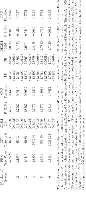
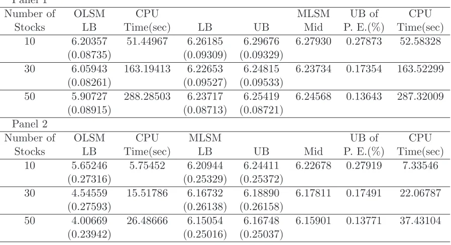
Example 2. American arithmetic average options on 10, 30 and 50 underlying assets following MJD processes.

To further demonstrate the performance of MLSM, we consider American arith-metic average options with underlying assets following the Merton-Jump-Diffusion process, where the jumps are assumed to be co-jump as conventionally adopted in the literature. In particular, the co-jump component parameters are set to be λ = 5, J ∼ N(−0.1,0.1) and σi2 = 1 for all i = 1, ..., n.14 Moreover, we

increase the number of underlying assets to 10, 30 and 50 with parameters of diffusion components remaining the same as in Example 1. If not otherwise mentioned, the we stick to the same parameters as in Example 1 for consis-tency. The results are presented in Table 2.2, where Panel 1 and 2 summarize results simulated with M = 10000 and M = 1000, respectively15_.

As Panel 1 illustrates, MLSM generates good approximations for the true values with upper bounds of pricing errors (UB of P. E.) up to 0.278%. By contrast, the lower bounds obtained by OLSM are consistently lower than those by MLSM. In particular, it is approximately 5% lower for the 50-asset case. Moreover, MLSM provides both lower and upper bounds with the similar computational time. Besides, Panel 2 indicates the efficiency of MSLM, in terms of the MC paths required. More specifically, with 1/10 MC paths, MLSM generates quan-titatively similar results with around 3 times larger standard deviation in com-parison with those in Panel 1. OLSM, however, provides even 50% smaller lower bound for 50-asset case relative to the one obtained by MLSM. The rea-son for this is that the geometric average approximate the arithmetic average

14

For illustrative purpose, we setσi2 = 1 for all i=1,...,n. We also tried the cases where the

underlying assets are allowed to have different sensitivities to the co-jump, i.e. σi2 varies

across different underlying assets. Consistently, MLSM yields good results.

15

(34)

accurately and, compared to OLSM, MLSM has only three parameters to be estimated for determining the exercise value the American geometric average option at each step.

Example 3. Simultaneous perturbation stochastic approximation (SPSA) benchmarking

The upper bounds implied by MLSM hinges on the key inequality, (2.11), where the latter term is essentially an American geometric average option and esti-mated by MLSM in the numerical experiments. Essentially, this American geo-metric average option would be estimated accurately by MLSM or OLSM since it is a 1-dimensional problem if stock prices are the only state variables. How-ever, to further demonstrate the applicability and accuracy of the estimation for this American geometric average option, we apply the Simultaneous pertur-bation stochastic approximation (SPSA)16_{for Example 1 as benchmark.}17 _The

parameters remains the same as in Example 1 except N which is set to be 4 for illustrative purpose.18 _{The set of SPSA parameters are:} _ak ₌ 100

(10+k)0.751 and

ck = _k010.25, where k denotes the kth iteration of total 500 iterations.(For details

about the SPSA algorithm and the parameters, see Fu et al (2000), Spall (1998) and among others.)

Table 2.3 indicates the accuracy of the MSLM algorithm. TheSP SAGA value column summarizes the American geometric average option values obtained by SPSA algorithm, while American GA column shows the geometric average op-tion values obtained by MLSM. As both columns illustrate, the values differ only in the third decimal points in all cases, which indeed imply the accuracy and validity of applying MSLM for estimating the American geometric aver-age option for constructing the MLSM upper bound. Besides, SP SAAA value column reports the values of American arithmetic average options obtained by SPSA algorithm. As the results indicate, SPSA algorithm provides reliable benchmark for American arithmetic average options with low number of exer-cise opportunities.

16

Please refer to Spall (2012) for details about SPSA algorithm

17

We thank an anonymous referee for the comments about applying the SPSA algorithm.

18

(35)

Example 4. American arithmetic average options on 30 underlying assets with 20 long and 10 short positions.

As mentioned in Section 2.1, the MLSM algorithm also applies to American arithmetic average options with both positive and negative weights. We pro-vide a concrete example here for completeness.19

More specifically, the exercise value of this option at timet _∈Γ can be expressed as

30

X

i=1

aiSit =

20

X

i=1

aiSit₋

30

X

i=21

(₋ai)Sit

The two arithmetic means are then approximated by their geometric means, denoted as GA+t andGA−t respectively, as illustrated in Step 1. Following this, the dimension of the pricing problem is reduced to two for MLSM algorithm. Accordingly, the cross sectional regression for MLSM is now applied with basis functions 1, GA+t , GA−t, GA+t ×GA−t ,(GA+t )2,(GA−t)2 here, while OLSM is im-plemented as in other examples. With respect to the parameters, they are kept the same as in Example 1 except that we increase the number of underlying assets to 30, where 20 assets are allocated with positive weights and the others are with negative weights and vary the strike price, K, from 34 to 37.20 _The

results are summarized in Table 2.4.

As Panel 1 shows, MLSM generates higher lower bounds in comparison with OLSM and the accuracy of MLSM are reflected by the upper bounds of pricing errors, which are below 1% except for K=34. Moreover, the simulation is re-peated withM = 1000 and the results are reported in Panel 2. Consistent with previous examples, the efficiency of MSLM in terms of MC paths required is pre-served for the case with both positive and negative weights. In contrast, OLSM generates significantly smaller lower bounds (around 11.5% lower as K=34).

Example 5. American arithmetic average options on 20 and 30 un-derlying assets with different volatilities.

In this example, to show that MLSM is applicable in general, we consider two models of 20 and 30 underlying assets with prices following GBM with variety in volatilities. The closeness between arithmetic and geometric averages

de-19

We thank an anonymous referee for pointing out this to improve the completeness of the paper.

20

(36)

pends on volatility. To examine the effect of volatility on pricing accuracy, we change the volatilities of the underlying assets with other parameters remain-ing the same as in previous examples. The results obtained with N=50 and M0 = 1000, M = 10000 are summarized in Table 2.5. In Panel 1, the

volatil-ities are set to be σi1 = 0.15, i = 1, ...,10;σi1 = 0.2, i = 11, ...,20 for 20-asset

case and σi1 = 0.1, i= 1, ...,10;σi1 = 0.15, i= 11, ...,20, σi1 = 0.2, i= 21, ...,30

for 30-asset case.

As this table indicates, OLSM provides lower bounds around 1% lower than MLSM. The accuracy of MLSM is reflected by the upper bounds of pricing errors around 0.6% for both cases. Moreover, when the volatility structures among the underlying assets are changed toσi1 = 0.15, i= 1, ...,10;σi1 = 0.3, i= 11, ...,20

for 20-asset case and σi1 = 0.15, i = 1, ...,10;σi1 = 0.2, i = 11, ...,20, σi1 =

0.3, i = 21, ...,30 for 30-asset case with other parameters unchanged to allow more variations in the price processes, Panel 2 shows that MLSM consistently generate higher lower bounds with small upper bounds of pricing errors around 1.067% and 0.821% for both cases respectively.

Similarly, the simulations are repeated withM = 1000 and summarized in Panel 3 and 4 to show the convergency speed of MLSM in terms of MC paths required. Both Panel 3 and 4 show that the results obtained by MLSM are quantitatively the same; however, those obtained by OLSM are significantly underestimated. In the worst case (the last row), the lower bound (2.282) is approximately 21% lower than the one obtained by MLSM (2.765).

Example 6. American arithmetic average options on 10 and 20 un-derlying assets following Heston’s model.

In this example, we consider Heston’s model (1993) of stochastic volatility to demonstrate the performance of MLSM for pricing American arithmetic average options. For the stock i, its price Sit and variance σ2it are given by:

dSit =rSitdt+σitdW_its,

dσ_it2 =α(β₋σ_it2)dt+γσitdW_itv, i= 1, ..., n,

whereWv

it, i= 1, ..., nare independent Brownian motions, that is, volatility pro-cesses are independent; for the stocki, the Brownian motions Ws

it and Witv are correlated with coefficients, ρi, i= 1, ..., n, capturing leverage effect; for i 6=j, Ws

it and Wjts are correlated with a coefficientρij, namely, the stock returns are correlated .

(37)

volatility processes as state variables, which should be included in the cross sec-tional regression. Considering the case of 10 stocks, a geometric mean, denoted as GAt, depends on 11 state variables, that is, the geometric mean itself and the 10 stochastic volatility processes. In contrast, the original arithmetic mean depends on 20 state variables, that is, the 10 stock price processes and the 10 stochastic volatility processes. More specifically, the basis functions adopted in this example for MLSM are: 1, GAt, GA2

t, σit, σit2, i = 1, ...,10/20; for OLSM: 1, Sit, S2

it, σit, σit2, i= 1, ...,10/20.

In this exercise, we only present lower bound estimates since the true values of American geometric average options are not easy to obtained for upper bounds due to higher dimension. The simulation results are summarized in Table 2.6. Compared with OLSM, MLSM still provides an effective way to estimate lower bounds. As Panel 1 shows, MLSM generate higher lower bounds for both cases compared to those obtained from OLSM. Moreover, Panel 2 further manifests the performance of MLSM by reducing M to 2500.21 _{More concretely, the}

results obtained by MLSM are quantitatively similar to those in Panel 1. In contrast, OLSM generates significantly lower estimates compared with the re-sults asM = 10000.

To show the results are not subject to the specific second-order basis function adopted, we repeat the simulation by increasing the order of basis functions to four and summarize the results in Panel 3.22 _{As Panel 3 demonstrates, MLSM}

generates consistent results as in Panel 1; however, the estimates by OLSM deteriorate around 1 to 2 %.

Example 7. Convergence comparisons of MLSM and OLSM.

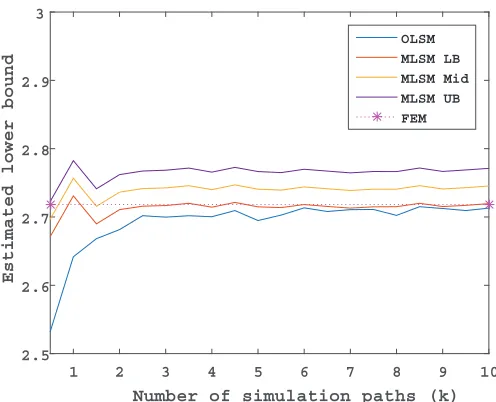
In this exercise, we repeat the 6-asset case in Example 1 to examine the rate of convergence for OLSM and MLSM by varying the number of simulation paths from 500 to 10000. The results are displayed in Figure 2.2. The lower bounds estimated by MLSM are consistently higher than those by OLSM. Moreover, the estimates obtained by the former start to approach the benchmark value (2.71838) essentially bounded below after the number of simulation paths ex-ceeds 1000. By contrast, the lower bound estimates from OLSM converge much slower than the MLSM estimates. In particular, 10000 simulation paths are

21

Since the number of state variables increases as volatilities are allowed to be stochastic, the pricing problem for MSLM is not one dimensional for this example anymore. As a result, it requires more MC paths (2500) in comparison with 1000 paths as analyzed in the previous examples.

22

(38)

Number of simulation paths (k)

1 2 3 4 5 6 7 8 9 10

Estimated lower bound

2.5 2.6 2.7 2.8 2.9 3

[image:38.595.184.432.109.310.2]

OLSM MLSM LB MLSM Mid MLSM UB FEM

Figure 2.2: Comparison of convergence speeds of MLSM and OLSM for pricing American arithmetic average option on 6 assets

sufficient for a good lower bound estimate. It is also noteworthy that the upper bound estimate from MLSM converges very fast too, in the sense that it con-verges to the true upper bound implied by MLSM as indicated by Figure 2.2. The desirable efficiency of MLSM arises from two key facts. Firstly, the arith-metic mean can be accurately approximated with the corresponding geometric mean. Secondly, the pricing problem for MLSM is reduced to lower dimension and or even 1 dimension for the case where the underlying assets follow the deterministic GBM process in particular.

Example 8. Robustness test for MLSM and OLSM with SPSA as benchmark23

As demonstrated in (2.7), the MLSM is especially efficient when the volatility and the time-to-maturity are not very high. In this example, we test per-formance of our MLSM in cases where volatility and/or time-to-maturity are relatively high.24 _{More specifically, American arithmetic average options on 10}

assets with the time-to-maturity and the volatility ranging from 0.5 years to 5 years and 0.15 to 0.5, respectively, are investigated with other parameters fixed as in Example 3.25 _{SPSA is adopted as a reasonable benchmark, i.e., true value,}

23

FEM method is a PDE-based algorithm and is hard to get accurate prices in high dimensional cases. As a result, we apply SPSA as the main benchmark here as discussed in Example 3.

24

We are very grateful to an anonymous referee for suggesting this test.

25

(39)

here as justified in Example 3.

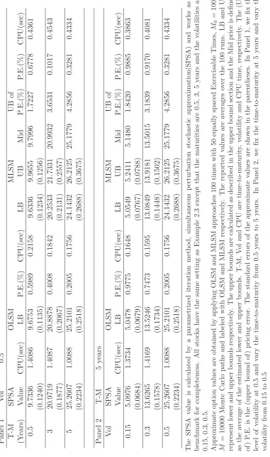
First, we investigate the effect of high-volatility case by fixing the level of volatil-ity at 0.5 and vary the time-to-maturvolatil-ity from 0.5 years to 5 years. Then, we fix the time-to-maturity at 5 years and vary the volatility from 0.15 to 0.5 to illustrate the effect of long time-to-maturity. The results of both cases are summarized in the upper and bottom panels of Table 2.7, respectively. As sum-marized in the table, MLSM provides lower lower bounds relative to the OLSM estimators in high-volatility and long time-to-maturity cases and higher upper bounds of pricing errors relative to those in Examples 1 to 7. In particular, the upper bounds of pricing errors are as high 4.2856% when the volatility is 0.5 and the time-to-maturity is equal to 5 years. However, as the column under “P. E.” indicates that MLSM provides good estimators given by the mid prices for American arithmetic average options in terms of pricing errors with SPSA esti-mators as benchmark. This finding is consistent with our result (2.12) that the upper bounds of pricing errors are conservative estimators of true pricing errors.

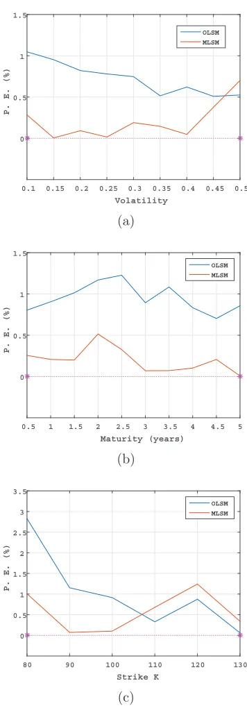
Furthermore, we test the performance of MLSM by varying volatility, time-to-maturity and strike price, respectively.26 _{In the following tests plotted in}

Figure 3, we graphically illustrate the pricing errors (P.E.) with SPSA estima-tors as benchmark and number of simulation path, M=10000. Specifically, in Panel (a), we vary volatility with time-to-maturity fixed at 1 year and other parameters fixed as in Example 3; in Panel (b), we vary time-to-maturity with volatility fixed at 0.2 and other parameters fixed as in Example 3; in Panel (c), with time-to-maturity fixed at 1 year, volatility fixed at 0.5 and other parame-ters fixed as in Example 3, we test performance of MLSM against different strike prices by scaling the strike price by exp(rT +a√T) with a ranging from -1/4 to 1/4. As Figure 2.3 demonstrates, reflected by “P. E.”, mid prices obtained by MLSM are good estimators for American arithmetic average options among a reasonable range of time-to-maturities, volatilities, and strike prices.

26

(40)

(41)

Volatility

0.1 0.15 0.2 0.25 0.3 0.35 0.4 0.45 0.5

P. E. (%)

0 0.5 1 1.5

OLSM MLSM

(a)

Maturity (years)

0.5 1 1.5 2 2.5 3 3.5 4 4.5 5

P. E. (%)

0 0.5 1 1.5

OLSM MLSM

(b)

Strike K

80 90 100 110 120 130

P. E. (%)

0 0.5 1 1.5 2 2.5 3 3.5

OLSM MLSM

[image:41.595.221.399.127.637.2]

(c)

Figure 2.3: Effects of volatility, time-to-maturity and strike price on pricing error. All stocks have the same setting as Example 2.3, i.e., Common Initial PriceSi0 = 100, Strike Price K=100, Interest rate r=3%, no Dividend, Maturity

(42)

[image:42.595.157.449.105.767.2]

(43)

Panel 1

Number of OLSM CPU MLSM UB of CPU Stocks LB Time(sec) LB UB Mid P. E.(%) Time(sec)

10 6.20357 51.44967 6.26185 6.29676 6.27930 0.27873 52.58328 (0.08735) (0.09309) (0.09329)

30 6.05943 163.19413 6.22653 6.24815 6.23734 0.17354 163.52299 (0.08261) (0.09527) (0.09533)

50 5.90727 288.28503 6.23717 6.25419 6.24568 0.13643 287.32009 (0.08915) (0.08713) (0.08721)

Panel 2

Number of OLSM CPU MLSM UB of CPU Stocks LB Time(sec) LB UB Mid P. E.(%) Time(sec)

10 5.65246 5.75452 6.20944 6.24411 6.22678 0.27919 7.33546 (0.27316) (0.25329) (0.25372)

30 4.54559 15.51786 6.16732 6.18890 6.17811 0.17491 22.06787 (0.27593) (0.26138) (0.26158)

50 4.00669 26.48666 6.15054 6.16748 6.15901 0.13771 37.43104 (0.23942) (0.25016) (0.25037)

The underlying stocks are modeled to follow MJD process with co-jump component

pa-rameters: λ= 5, J ∼N(−0.1,0.1). The other parameters in the models are : Common

Initial pricesSi0= 100, Strike Price K=100, Interest Rate r=3%, no Dividend, Common

volatilities σi1 = 20%, Common Correlationρ_ij = 0.5, i6=j = 1, ...,10/30/50 and

matu-rity, T is set to be 0.25 Year respectively. The jump sensitivities,σi2 to the jump are set

to be 1 for all underlying assets.

Approximate option values are obtained by applying OLSM and MLSM approaches 100

times for each case with 50 equally spaced Exercisable times, M0 = 1000, M = 10000

Monte Carlo paths and labeled with OLSM and MLSM, respectively in Panel 1. In

contrast, the simulation is repeated withM = 1000 to examine the efficiency against the

[image:43.595.115.564.197.441.2]

number of the Monte Carlo paths. The results are reported in the Panel 2. The reported values are averages over the 100 runs. LB and UB represent lower and upper bounds, respectively. The upper bounds are calculated as described in the upper bound section and the Mid is defined as the average of the estimated lower and upper bounds. The UB of P. E. is the upper bound of pricing error. The standard errors of the approximate values are shown in the parentheses.

(44)

[image:44.595.134.477.114.750.2]

(45)

Panel 1

Strike LSM MLSM UB of Price LB LB UB Mid P. E.(%)

34 1.30585 1.31802 1.34946 1.33374 1.19289 (0.01544) (0.01356) (0.01364)

35 1.96168 1.97742 2.01409 1.99575 0.92709 (0.01525) (0.01411) (0.01414)

36 2.75018 2.77325 2.81316 2.79320 0.71944 (0.01431) (0.01685) (0.01699)

37 3.65444 3.67401 3.71595 3.69498 0.57079 (0.01288) (0.01365) (0.01376)

Panel 2

34 1.16107 1.29531 1.32679 1.31105 1.21501 (0.04149) (0.04743) 0.04763

35 1.83902 1.97582 2.01240 1.99411 0.92558 (0.04853) (0.04697) 0.04721

36 2.68046 2.76171 2.80173 2.78172 0.72459 (0.04248) (0.04859) 0.04864

37 3.61886 3.65690 3.69850 3.67770 0.56879 (0.04049) (0.04741) 0.04747

In this table, the applicability of MLSM for portfolios composed of both long and short

positions, i.e. positive and negative weights is examined. In particular, ai = 1/30, for

i= 1, ...,20 andai=−1/30, fori= 21, ...,30. The parameters in the model are : Common

Initial pricesSi0= 100, i= 1, ...,30, Interest Rate r=3%, no Dividend, Maturity T=0.25

Year, Common Correlation ρij = 0.5, i 6=j = 1, ...,30. The results are summarized as

K=34,...,37 for illustration. The computational times for LSM and MLSM are around 20 and 18, respectively and not reported in the table for illustrative brevity.

Approximate option values are obtained by applying OLSM and MLSM approaches 100

times for each case with 50 equally spaced Exercisable times, M0 = 1000, M = 10000

Monte Carlo paths and labeled with OLSM and MLSM respectively in Panel 1. In

con-trast, the simulation is repeated with M = 1000 to examine the efficiency against the

[image:45.595.155.472.175.447.2]

number of the Monte Carlo path. The results are reported in the Panel 2. The reported values are averages over the 100 runs. LB and UB represent lower and upper bounds respectively. The upper bounds are calculated as described in the upper bound section and the Mid is defined as the average of the estimated lower and upper bounds. The UB of P. E. is the upper bound of pricing error. The standard errors of the approximate values are shown in the parentheses.