On extended state space constructions for monte carlo methods

(1)

A Thesis Submitted for the Degree of PhD at the University of Warwick

http://go.warwick.ac.uk/wrap/77119

This thesis is made available online and is protected by original copyright. Please scroll down to view the document itself.

(2)

Axel Finke

On

Extended State-Space

Constructions

for

Monte Carlo Methods

Thesis submitted for the degree of

Doctor of Philosophy

(3)

(4)

(5)

(6)

Summary

This thesis develops computationally efficient methodology in two areas. Firstly, we consider a particularly challenging class of discretely observed continuous-time point-process models. For these, we analyse and im-prove an existing filtering algorithm based on sequential Monte Carlo

(

smc

) methods. To estimate the static parameters in such models, we devise novel particle Gibbs samplers. One of these exploits a sophisticated non-centred parametrisation whose benefits in a Markov chain Monte Carlo(

mcmc

) context have previously been limited by the lack of

block-wise updates for the latent point process. We apply this algorithm to a Lévy-driven stochastic volatility model. Secondly, we devise novel Monte Carlo methods – based around pseudo-marginal and conditional

smc

approaches – for performing optimisation in latent-variable models and more generally. To ease the explanation of the wide range of techniques employed in this work, we describe a generic importance-sampling frame-work which admits virtually all Monte Carlo methods, including

smc

and

mcmc

methods, as special cases. Indeed, hierarchical combinations of different Monte Carlo schemes such as

smc

within

mcmc

or

smc

within

(7)

(8)

Declaration

This thesis is the result of my own work and research, except where otherwise indicated. Chapter 4 is a condensed version of the published journal article

Finke, A., Johansen, A. M. & Spanò, D. (2014). Static-param-eter estimation in piecewise dStatic-param-eterministic processes using particle Gibbs samplers. Annals of the Institute of Statistical Mathematics,66(3), 577–609.

This thesis has not been submitted for examination to any other institution than the University of Warwick.

(9)

(10)

Acknowledgements

There are many people without whom I could not have written this thesis or undertaken the research on which it is based.

First, I would like to thank my supervisors, Adam M. Johansen and Dario Spanò, for their patience, guidance, refreshing sarcasm, and con-stant support throughout the past three-and-a-half years. I consider myself extremely fortunate for the substantial amount of enthusiasm and intuition for Monte Carlo methods they have bestowed upon me.

For significantly improving the presentation of this thesis, in particular of Chapters 1, 3 and 6, I am indebted to my other proofreaders: Cyril Chimisov, Andreas L. Hetland, and Felipe Medina-Aguayo.

I have benefited immensely from stimulating discussions with my col-leagues (in no particular order): Murray Pollock, Giacomo Zanella, and Kirsty Hey, for which I am deeply grateful. I would also like acknowledge all the other participants of the Feynman–Kac and Markov chain Monte Carlo reading groups, and the various other seminars on computational statistics at Warwick. By furthering my understanding of the topic, they have all, in some way, contributed to this thesis.

I would also like to thank Gareth O. Roberts and Nick Whiteley for taking the time to read and examine my thesis and for taking an interest in my research.

Furthermore, I wish to express my thanks to Professor Mark Trede for introducing me to computational statistics and for encouraging me to study in the

uk

.

This work was also generously supported by Engineering and Physical Sciences Research Council Doctoral Training Grant

ep/j500586/1

.

(11)

(12)

I

Generic Monte Carlo Framework

1 Elementary Monte Carlo Tools 1 1.1 Importance Sampling . . . 1

1.1.1 Motivation . . . 1

1.1.2 Change of Measure . . . 2

1.1.3 Sampling-Based Approximation . . . 2

1.1.4 Theoretical Properties . . . 3

1.2 Self-Normalised Importance Sampling . . . 4

1.2.2 Sampling-Based Approximation . . . 5

1.2.3 Theoretical Properties . . . 5

1.2.4 Effective Sample Size . . . 6

1.3 State-Space Extension and Reduction . . . 7

1.3.1 Enlarging the Space . . . 7

1.3.2 Importance Sampling on the Joint Space . . . 8

1.3.3 Rao–Blackwellisation . . . 9

1.3.4 Examples . . . 10

1.4 Marginalised One-Sample Importance Sampling . . . 13

1.4.1 Extended Target Measure . . . 13

1.4.2 Generic Estimator . . . 15

1.4.3 Pseudo-Marginal Interpretation . . . 17

1.4.4 Application to Standard Importance Sampling . . 19

(13)

2 Sequential Monte Carlo Methods 23

2.1 Introduction . . . 23

2.1.2 Particles and Parent Indices . . . 25

2.1.3 Resampling . . . 26

2.1.4 Generic Algorithm . . . 28

2.2 Interpretation as Importance Sampling . . . 29

2.2.1 Extended Proposal Distribution . . . 29

2.2.2 Extended Target Measure . . . 31

2.2.3 Importance Weights . . . 33

2.2.4 Rao–Blackwellisation . . . 35

2.2.5 Theoretical Results . . . 36

2.3 Some Important

smc

Algorithms . . . 38

2.3.1 Simple

sir

Algorithm . . . 38

2.3.2

smc

Samplers . . . 41

2.3.3 Re-Using All Particles . . . 44

2.3.4 Discrete Particle Filter . . . 49

2.3.5 Other

smc

Algorithms . . . 51

2.4 Sample Impoverishment and Remedies . . . 52

2.4.1 Particle-Path Coalescence . . . 52

2.4.2 Backward Smoothing . . . 53

2.4.3 Backward Sampling . . . 57

2.5 Summary . . . 57

3 Markov Chain Monte Carlo Methods 59 3.1 Introduction . . . 59

3.1.2 Note on Ergodicity . . . 60

3.1.3 Generic Algorithm . . . 61

3.1.4 Interpretation as Importance Sampling . . . 62

3.2 Generic

mcmc

Kernel . . . 64

3.2.1 Elementary Kernels . . . 64

3.2.2 Combinations of Kernels . . . 65

3.2.3 Generic

mcmc

Kernel . . . 66

3.2.4 Finite State-Space Kernels . . . 69

3.3 General State-Space Kernels . . . 71

(14)

Contents

3.3.2 Reversible-Jump

mcmc

. . . 75

3.3.3 Randomised

mcmc

. . . 76

3.3.4 Pseudo-Marginal

mcmc

. . . 79

3.3.5 Ensemble

mcmc

. . . 82

3.4 Conditional

smc

Kernels . . . 87

3.4.1 Iterated

csmc

Kernel . . . 87

3.4.2 Variance-Reduction Techniques . . . 89

3.4.3 Duality of Backward and Ancestor Sampling . . . 92

3.4.4 Application to Particle Gibbs Samplers . . . 95

3.5 Summary . . . 98

II

Some Novel Monte Carlo Schemes

4 Inference in Piecewise Deterministic Processes 103 4.1 Introduction . . . 103

4.1.1 Motivation . . . 103

4.1.2 Contribution . . . 104

4.2 Piecewise Deterministic Processes . . . 105

4.2.1 Definition . . . 105

4.2.2 Elementary Change-Point Example . . . 107

4.2.3 Shot-Noise Cox-Process Example . . . 108

4.2.4 Object-Tracking Example . . . 110

4.3 Existing

smc

Algorithms . . . 111

4.3.1 Variable-Rate Particle Filter . . . 111

4.3.2

smc

Filter for

pdp

s . . . 114

4.3.3 Theoretical Analysis . . . 116

4.4 Reformulation of the

smc

Filter . . . 121

4.4.1 General Idea . . . 121

4.4.2 Extended Target Distribution . . . 121

4.4.3 Extended Proposal Distribution . . . 124

4.4.4 Distribution Over Birth-Move Locations . . . 125

4.4.5 Incremental and Backward-Sampling Weights . . 126

4.4.6 The Algorithm . . . 128

4.5 Simulation study . . . 130

4.5.1 General Setup . . . 130

(15)

4.5.3 Shot-Noise Cox-Process Model . . . 133

4.6 Summary . . . 135

5 Particle Gibbs Samplers for Poisson-Process Models 137 5.1 Introduction . . . 137

5.1.1 Motivation . . . 137

5.2 Non-Centred Metropolis-Within-Gibbs Algorithm . . . . 139

5.2.1 Actual Target Distribution . . . 139

5.2.2 Non-Centred Parametrisation . . . 140

5.2.3 Extended Target Distribution . . . 143

5.2.4 The Algorithm . . . 144

5.3 Non-Centred Particle Gibbs Sampler . . . 145

5.3.1 Motivation . . . 145

5.3.2 Conditional

smc

Kernel . . . 146

5.3.3 Full Algorithm . . . 148

5.4 Application to Lévy-Driven Stochastic Volatility Models . 149 5.4.1 Model Description . . . 149

5.4.2 Choice of Priors . . . 150

5.4.3 Algorithm Details . . . 151

5.4.4 Simulation Study . . . 153

5.5 Summary . . . 158

6 Pseudo-Marginal Monte Carlo Optimisation 161 6.1 Introduction . . . 161

6.1.1 Motivation . . . 161

6.2 Background . . . 164

6.2.1 Simulated Annealing . . . 164

6.2.2 State Augmentation for Marginal Estimation . . . 164

6.2.3 Optimisation Using

smc

Samplers . . . 167

6.3 Novel Methodology . . . 169

6.3.1 Pseudo Gibbs Samplers . . . 169

6.3.2 Pseudo-Marginal Optimisation . . . 171

6.3.3 Incorporation Into

smc

Samplers . . . 175

6.4 Applications . . . 175

(16)

Contents

6.4.2 Linear Gaussian State-Space Model . . . 178

6.4.3 Simple Stochastic Volatility Model . . . 182

6.5 Discussion . . . 186

Conclusion 189 Summary . . . 189

Contributions . . . 190

Future Directions . . . 193

A Resampling Schemes 195 A.1 Overview . . . 195

A.2 Multinomial Resampling . . . 195

A.3 Stratified Resampling . . . 196

A.4 Systematic Resampling . . . 197

A.5 Optimal Finite-State Resampling . . . 197

Notation 201

Abbreviations 203

(17)

(18)

List of Figures

1.1 Relationship between various Monte Carlo schemes . . . 21

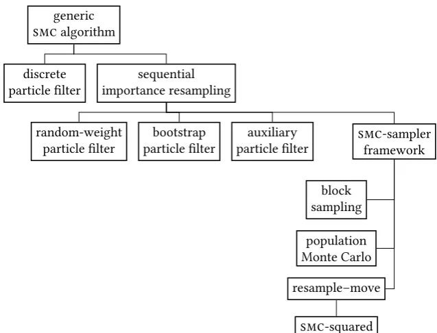
2.1 Relationship between various

smc

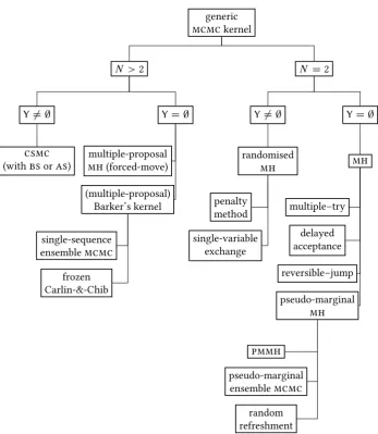
algorithms . . . 58

3.1 Relationship between various

mcmc

kernels . . . 99

4.1 Data simulated from the change-point model . . . 108

4.2 Data simulated from the Cox-process model . . . 110

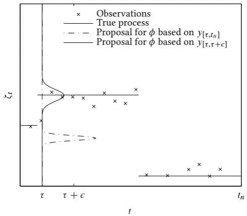
4.3 Jump-size proposal distributions for

pdp

s . . . 118

4.4 Static-parameter estimates for the change-point model . 134 4.5 Traces for the simple change-point model . . . 135

4.6 Static-parameter estimates for the Cox-process model . . 136

5.1 Parameter estimates in one-component Lévy-driven stochastic volatility models . . . 156

5.2 Autocorrelation of the parameter estimates in one-component Lévy-driven stochastic volatility models . . . 157

5.3 Parameter estimates in two-component Lévy-driven stochastic volatility models . . . 159

5.4 Autocorrelation of the parameter estimates in two-component Lévy-driven stochastic volatility models . . . 160

6.1 Loglikelihood in the Student-t toy model . . . 176

6.2 Traces in the Student-t toy model . . . 179

6.3

ml

estimates for the Student-t toy model . . . 180

6.4 Traces for the linear Gaussian

hmm

. . . 183

6.5

ml

estimates for the linear Gaussian

hmm

. . . 184

(19)

(20)

Introduction

Context

Since its invention in the 1940s, the idea of approximating integrals by random samples, known as the Monte Carlo method, has served as a vital tool for scientific discovery in a wide range of disciplines such as biology (Wilkinson, 2011), econometrics (Greenberg, 2012; Durbin & Koop-man, 2012), engineering (Cappé, Moulines & Rydén, 2005), epidemiology (Gibson & Renshaw, 1998; O’Neill & Roberts, 1999), operations research (Fishman, 1996), physics (Spanier & Gelbard, 1969; Sokal, 1997; Lapeyre, Pardoux & Sentis, 2003), and political science (Gelman et al., 2013)

In addition, the Monte Carlo method has spurred technological pro-gress appreciable in everyday life. For instance, it now aids the tracking and positioning of mobile robots (Dellaert, Fox, Burgard & Thrun, 1999), produces weather forecasts (Epstein, 1969; Leith, 1974), predicts elec-tions (‘FiveThirtyEight’, 2015), prices complicated financial instruments (Glasserman, 2004), and generates visual effects in blockbuster movies from animation studios such as Pixar (Veach & Guibas, 1995; Lokovic & Veach, 2000) – even leading to a Technical Oscar for Thomas Lokovic and Eric Veach (‘The 86th Scientific & Technical Awards’, 2014).

This thesis is largely concerned with developing sophisticated instances of the Monte Carlo method tailored to particular challenging real-world problems. To that end, we combine, extend, and improve a number of existing algorithms. As a by-product, we provide a unifying Monte Carlo framework which admits new insight into the relationship between the vast array of complex Monte Carlo algorithms that exist today.

(21)

Outline

This thesis is divided into two parts. Part I provides some background on various Monte Carlo algorithms. Novel methodology is mostly, but not exclusively, confined to Part II.

Part I. In the first part, we briefly review basic Monte Carlo methodology,

such asimportance sampling(

is

),sequential Monte Carlo(

smc

) methods,

andMarkov chain Monte Carlo(

mcmc

) methods. To provide the reader

with a better intuition for such a plethora of techniques, we present a gen-eric

is

framework, best described asmarginalised one-sample importance sampling (

mosis

), which admits essentially all instances of the Monte

Carlo method, including those mentioned above, as special cases.

Chapter 1 reviews

is

as a particularly useful interpretation of the Monte

Carlo method. We also describe self-normalised

is

as well as state-space extension and state-space reduction techniques. Combining these ideas, we then develop the generic

mosis

framework which forms the heart of any Monte Carlo algorithm. We also show that this framework can, for instance, be used to justify pseudo-marginal approaches.

Chapter 2 devises a generic

smc

scheme and demonstrates that it admits

essentially any

smc

algorithm as a special case, including, for instance, the discrete particle filter which could hitherto not be viewed as a stand-ard

smc

algorithm. In turn, we show that the generic

smc

algorithm is itself a special case of

mosis

. In addition, we generalise and improve existing schemes which approximate integrals by recycling all particles generated by an

smc

sampler.

Chapter 3 shows that

mcmc

methods, too, can be viewed as

mosis

and

that a repeated, hierarchical application of

mosis

forms the basis of all

mcmc

kernels, including pseudo-marginal, randomised, and ensemble

(22)

Notation

Part II. In the second part, we develop novel Monte Carlo methodology

for two problems. Firstly, we devise methods for filtering and static-parameter estimation in a class of discretely observed continuous-time piecewise deterministic processes. These may also be viewed as partially-observed point processes. Secondly, we construct efficient Monte Carlo algorithms for optimisation in latent-variable models and more generally.

Chapter 4 motivates the use of piecewise deterministic processes and

reviews, analyses and improves an existing

smc

-based filter for such models. Around it, we also devise a particle Gibbs sampler – with a novel auxiliary-variable rejuvenation step – to perform static-parameter estimation.

Chapter 5 considers static-parameter estimation in partially-observed

piecewise deterministic processes driven by compound Poisson pro-cesses. To improve mixing of the particle Gibbs chain, we adopt a non-centred parametrisation. The resulting algorithm is applied to a particularly challenging Lévy-driven stochastic volatility model.

Chapter 6 develops a framework for performing optimisation, e.g. for

maximum likelihood or maximum a-posteriori estimation in latent-variable models. Specifically, we devise generic

smc

and

mcmc

optim-isation schemes within which sophisticated Monte Carlo approaches such as pseudo-marginal methods or particle Gibbs samplers can be incorporated.

A detailed list of novel contributions can be found on Page 190.

Notation

It may be helpful to clarify some notational conventions used throughout this work although non-standard notation is also explained in the main text on the first use. For easy reference, we also provide a list of frequently used symbols on Page 201 along with a list of acronyms on Page 203.

Sets. We denote byRZN, respectively, the sets of real numbers,

integers and positive integers. We often make use of the following subsets of the latter two: Zk;l WD fz 2 Z j k z lg and Nl WD Z₁;l.

Furthermore, #Adenotes the cardinality of some countable setA. Finally, A₁_W_nWD

pnD1Ap WDA1 An represents the Cartesian product of

(23)

Vectors. We write x1_tWN WD.x_t1; : : : ; xN_t /and xn

1WT WD.x n

1; : : : ; xTn/. To

avoid ambiguity, we often use the bold face notation xt WDx1tWN when

both sub- and superscripts need to be vector valued. In this case, we often letx_tk _WD.x1tWk 1; x

kC1WN

t /be the vectorxwithout itskth component.

Finally,ATdenotes the transpose of some matrixA.

Measures. All measures considered in this work will be positive. We

writeM¢.X/M.X/ M₁.X/for the sets of (positive)¢-finite, finite,

and probability measures on some measurable space.X;X/. Whenever

possible, we take,X DWB.X/, whereB.X/is the Borel¢-algebra onX.

In this case, we refer to elements of the above-mentioned sets as measures ‘onX’. In particular, Leb 2 M¢.R/denotes the Lebesgue measure on

R. For; 2 M¢.X/, we write if absolutely continuous with

respect toand in this case, d=ddenotes the corresponding Radon–

Nikodým derivative, i.e. D Œd=d. It is sometimes convenient to

abuse the notation for Radon–Nikodým derivatives and to alternatively writeŒd=d.x/DW.dx/=.dx/.

Functions. For measurable spaces.X;X/and.Y;Y/, endowed with

suit-able¢-algebrasXandY, we define F.X;Y/_WD˚

f WX !Yˇˇf isX=Y-measurable :

Furthermore, we let idX 2F.X;X/denote the identity function and let

1B 2F.X;f0;1g/represent the indicator function ofB X, i.e.

1B.x/WD

(

1; ifx 2B,

0; ifx 2XnB.

IfB DX, we set1X DW1. For any functionf WX !Y, andB Y, the

preimage ofBunderf is denotedf 1.B/_{WD f}x 2X jf .x/2Bg. For

functionsf andg with domainXandY, respectively, we use the

tensor-product notation Œf ˝g.x; y/ _WD .f .x/; g.y//, for .x; y/ 2 X Y.

Furthermore, ifX DY, we writefg.x/_WDf .x/g.x/, forx 2X, as usual.

Integrals. For any2M_¢.X/and anyp 2Œ0;1/, we let

Lp./WD˚

f 2F.X;R/ˇˇ.jfjp/ <1

denote the set of p-times-integrable real-valued functions with the

convention that L1./ DW L./, and with the following convenient

shorthand for integrals: .f /WDR

(24)

Notation

Kernels. For measurable spaces.X;X/and.Y;Y/, a (positive)¢-finite

kernel is a functionKW XY !Œ0;1/if it satisfies both the following

properties:

8A2 YW K.; A/2 F.X; Œ0;1//; 8x 2XW K.x; /2 M¢.Y/:

We callK,finiteifK.x; / 2M.Y/, andstochastic ifK.x; /2 M₁.Y/,

for anyx 2 X. We denote byK¢.X;Y/ K.X;Y/ K₁.X;Y/the sets

of¢-finite, finite, and stochastic transition kernels from.X;X/to.Y;Y/.

For suitable kernelsK 2 K¢.X;Y/andL2 K¢.Y;Z/, we may define a

kernelK ˝L2K¢.X;YZ/by

ŒK ˝L.x; AB/_WDK.x;1AL.;1B//;

for all.x; A; B/2 XYZ, and define a kernelKL2 K¢.X;Z/by KL.x; B/WDŒK ˝L.x;YB/;

for all.x; B/2 XZ.

By extension, we setK₁˝_WnWD

Nn

pD1Kp WDK₁˝ ˝Kn, for suitable

kernels K₁; : : : ; Kn. In particular, if K1 D D Kn D K, we use the

shorthandK₁˝_WnDWK˝n.

The same conventions for (tensor)products apply to measures by view-ing them as kernels which are constant in their first argument. Finally, especially in Part II, we write a stochastic kernel K 2 K₁.X;Y/ as K.x;dy/DK.dyjx/, forx 2X. In particular, the distributionK.dyjx/

is then sometimes implicitly defined to be the full conditional distribution of the second component under the probability measureK 2 M₁.XY/.

Distributions. We generally work with some underlying probability

space.Ω;A;P/and letE;Vdenote expectation and variance under

some probability measure , with the convention that EP D E and

VP DV. Hence, for arandom variable X 2F.Ω;Rd/with distribution _WDP ıX 12M₁.X/, whereX 1.A/is the preimage ofAunderX, and

forf 2 L./, we have the usual identity.f / D EŒf D EŒf .X /.

For this work, important probability measures are N;˙, the normal

distribution with mean and covariance matrix ˙, and •x, the Dirac

measure or point mass centred at x, defined by•x.A/ WD 1A.x/. For a

(25)

(26)

Part I

Generic Monte Carlo

(27)

(28)

1 Elementary Monte Carlo Tools

1.1 Importance Sampling

1.1.1 Motivation

In this chapter, we describe tools that form the basis of all known Monte

Carlo algorithms. In Sections 1.1 and 1.2, we justify importance sampling and

self-normalised importance sampling. In Section 1.3, we describe state-space

extension techniques and also ways of reducing the dimension of the state

space (i.e. Rao–Blackwellisation). Finally, Section 1.4 combines the ideas

from the preceding sections into a generic importance-sampling framework

which admits essentially all known Monte Carlo schemes as a special case.

Let.Ω;A;P/be some probability space and letM.X/denote the set

of finite positive measures on some measurable space .X;B.X//. For 2M.X/, assume that we want to calculate integrals

.f /_WD Z

X

f d; (1.1)

for all test functionsf 2FL. / _{WD f}f W X!Rjf is-integrableg.

1.1 Remark. LetM_¢.X/denote the set of¢-finite (positive) measures on

.X;B.X//. Note that any finite integral .Q f /Q with respect toQ 2 M_¢.X/ may be written in the form of Equation1.1by applying the change of measure

_{WD Q}fQ (wherefQ .A/Q WD Q .fQ1_A/, forA2B.X/), and settingf 1.

Analytical computation of such integrals is often too costly or even impossible. Instead, numerical integration methods such as quadrature rules may be used. Unfortunately, the error of these methods is typically of orderO.N c=d_{), where}_d _{is the dimension of the state space}_X_,_{c >}_0,

andN is the number of grid points. The need forN to be exponentially

large in d is known as thecurse of dimensionality (Bellman, 1957). It

(29)

1.1.2 Change of Measure

To apply the methods developed in this work, we need to turn.f /into

an integral with respect some probability measure. This can always be achieved as follows. LetM₁.X/denote the set of probability measures on .X;B.X//and select 2M₁.X/such that . In this case,

.f /D .wf /DE Œwf ;

wherewdenotes the Radon–Nikodým derivativew WDd=d .

1.2 Remark. It suffices that f . However, we make the stronger requirement: , here because it is independent of the particular test function and we are usually concerned with approximating.f /for a large class of test functions,F.

1.1.3 Sampling-Based Approximation

Given a vector of independent and identically distributed (

iid

) draws

X _WDX1WN _from _{, (a suitable version of) the Glivenko–Cantelli theorem}

(Billingsley, 2012, Theorem 20.6) justifies using the empirical measure of these samples to approximate theprobability measure ,

mc;N

WD 1 N

N

X

nD1 •Xn:

Here,•x 2 M1.X/is the point mass (orDirac measure) located atx 2X.

We may thus approximate theintegral .f /D .wf /DE Œwf by

mc;N_{.wf /}

D Z

X

wf d mc;N D 1 N

N

X

nD1

wf .Xn/;

i.e. we estimate the expectation by the corresponding sample mean. Approximating integrals with respect to some probability measure in this way – usually by generatingX on a computer using pseudo-random

numbers – is known as theMonte Carlomethod. It was developed during

(30)

1.1 Importance Sampling

Project at the Los Alamos Scientific Laboratory, New Mexico. Some of the earliest available references include Goertzel and Kahn (1949), Metropolis and Ulam (1949). Historical accounts can be found in Metropolis (1987), Eckhard (1987), Rota (2008).

Note that we may also view the Monte Carlo method as a procedure for approximating themeasure by the following (random) unnormalised weighted empirical measure,

is;N _WD 1 N

N

X

nD1

w.Xn/•Xn;

wherew.Xn/is known as an unnormalisedimportance weight.

1.3 Remark. Throughout this work, for simplicity, we refer to the unnor-malised importance weights w.Xn/ simply as ‘weights’ or ‘importance weights’ and we refer to is;N as a ‘weighted empirical measure’, even thoughPN

nD1w.Xn/¤1, in general.

This view of the Monte Carlo method is known asimportance sampling(

is

)

(Goertzel & Kahn, 1949). Though, initially, it was also referred to asquota sampling (Goertzel, 1949). Plugging in the test function, it clearly leads to

the same estimator for.f /as above, i.e.is;N.f /D mc;N.wf /. One

of the goals of Part I of this work is to demonstrate that essentially every Monte Carlo algorithm can be seen as a special case of

is

which, in turn, is merely a convenient re-interpretation of the Monte Carlo method.

The

is

-interpretation of the Monte Carlo method is useful because we are usually concerned with approximating.f /for a large class of

test functions, F, but without selecting and sampling from a different

proposal distribution for eachf 2 Fas this tends to be costly. The

is

-interpretation helps separating the influence of the test functionf from

the influence of the proposal distribution on the estimatoris;N.f /

through the oscillations ofw.

1.1.4 Theoretical Properties

It is easy to see that is;N.f /is an unbiased estimator for .f / and

thestrong law of large numbers (

slln

) (Billingsley, 2012, Theorem 22.1)

(31)

set Li. / WD ff W X _! R _j fi is -integrableg. Ifwf 2 L2. /, so

that the asymptotic variance 2.f / WD VŒf exists, a simple central limit theorem(

clt

) (Billingsley, 2012, Theorem 27.1) guarantees that

p N

is;N.f / .f / N!1

! Z N0;2.f /;

in distribution. In particular, the Monte Carlo errorjis;N.f / .f /j

vanishes at a rateOP.N 1=2/which is independent of the dimensiond.

1.2 Self-Normalised Importance Sampling

1.2.1 Motivation

Assume that we wish to approximate.f /, for some probability measure 2 M₁.X/andf 2 L./. In many applications, the Radon–Nikodým

derivative wz WD d=d can only be evaluated up to some unknown

constantz>0. That is, we can evaluatew _WDzwz point-wise but notwz.

The intractability ofzrenders (standard)

is

inapplicable because we

can then only approximate the measure 2M.X/, defined by

WDw Dz

and ¤ , except in the trivial case that z D 1. Self-normalised

is

exploits fact that if is a probability measure thenz D .1/. Based

on this identity, we may use standard

is

to separately approximate the numerator and denominator in the identity D=zas described in the

next subsection.

We conclude this subsection by noting that the intractability ofzusually

arises because the target distribution or the proposal distribution are

constructed via non-linear transformations of some other measures onX.

More precisely, for2 M¢.X/andg 2L./, define theBoltzmann–Gibbs transformationofunderg,‰_g, by

‰g./ WDg=.g/:

Assume that is constructed via D‰g.$ /and is constructed via

D ‰h./, for some $; 2 M¢.X/, g 2 L.$ /, and h 2 L./. In

this case, we often have that z D $ .g/=.h/and this ratio is usually

(32)

1.2 Self-Normalised Importance Sampling

1.4 Example (Bayesian posterior). In Bayesian statistics, may be the posterior distribution given some prior distribution$and some dataywith associated likelihood g.Q ; y/ DW g D L, i.e. D ‰_L.$ /. The ‘model evidence’ or ‘marginal likelihood’,$ .L/, is then typically intractable.

1.2.2 Sampling-Based Approximation

The idea of self-normalised

is

is to separately approximate the numerator and denominator on the right hand side in the identity D =z via

standard

is

. That is, we approximate the measure by

is;N D 1 N

N

X

nD1

w.Xn/•Xn

and the integralzD.1/by

zis;N _WDis;N.1/D 1 N

N

X

nD1

w.Xn/:

LetWn.X/WDw.Xn/=zis;N denote thenthself-normalised importance weight. Combining the previous two approximations then defines the

self-normalised

is

approximation of,

is?; N D

is;N

zis;N D N

X

nD1

Wn.X/•Xn:

Again, we can approximate the integral.f /by

is?; N.f /D

N

X

nD1

Wn.X/f .Xn/:

1.2.3 Theoretical Properties

The estimatoris?; N.f /is biased but strongly consistent, i.e.is?; N.f /

converges almost surely to .f /, asN ! 1. As shown by Geweke

(1989), for instance, the estimator again satisfies a

clt

, i.e.

p N

is?; N.f / .f / N!1

(33)

in distribution, if we assume that w; wf 2L2. / to ensure that the

asymptotic variance2.f /WD.wŒfz .f /2/exists. More precisely,

Liu (2001, p. 35) proves that

Eis?; N.f /D.f /C .wŒfz .f //

N CO.N

2_/;

Vis?; N.f /D .wŒfz .f /

2_/

N CO.N

2_/:

In particular,zis;N is again an

is

estimate ofzand thus unbiased.

Finally, even though is?; N.f / is biased, its mean-square error can

sometimes be smaller than that of a standard

is

estimateis;N.f /

(as-suming thatwz can be evaluated). Intuitively, the former can obtain

vari-ance reductions by exploiting the fact that is a (random) probability

measure. Indeed,is?; N is a (random) probability measure butis;N is

not, in general, because its weights do not sum to 1.

1.2.4 Effective Sample Size

From the expression for the asymptotic variance2.f /above, it is clear

that the performance of self-normalised

is

is determined by how closely the target distribution resembles the proposal distribution , at least if

we neglect the contribution from the oscillations off.

Several criteria have been proposed to measure the efficiency of

is

approximations, such as theeffective sample size(

ess

), defined by Kong,

Liu and Wong (1994) as

ESS WD N

V .w/z C1 D Nz

.w/; (1.2)

ifwis-integrable. The effective sample size takes values in.0; N . If D thenwz 1 so thatESSDN. On the other hand,ESSdecreases

the more and differ.

Unfortunately, the

ess

cannot be calculated analytically because the difficulty of computing integrals of the form.w/is one of the reasons

for turning to importance sampling in the first place. We thus have to resort to estimating it by

ESSN WD

Nzis;N is?; N_.w/ D

ŒPN

nD1w.Xn/2

PN

mD1Œw.Xm/2

D _P_N 1

nD1ŒWn.X/2

(34)

1.3 State-Space Extension and Reduction

This estimate of the effective sample size ranges from 1 (all self-normalised importance weights are zero except one) toN (all importance weights

are identical).

Care must be taken when interpreting this estimate. For finiteN, it

is easy to construct examples in which the self-normalised

is

estimator has a high variance despite it being very likely that all self-normalised importance weights are roughly identical. This is the case if the proposal distribution is likely to miss high-probability regions under.

1.3 State-Space Extension and Reduction

1.3.1 Enlarging the Space

Assume again that we are interested in approximating (integrals with respect to) a measure 2M.X/by

is

, using some proposal distribution 2 M₁.X/such that . Sometimes, we cannot evaluate the Radon–

Nikodým derivative w _WD d=d point-wise – not even up to some

unknown proportionality constant. Thus, direct

is

approximations of

and, by extension, self-normalised

is

approximations of a probability

measure / are not available.

However, in some cases, the intractability of the importance weights can be circumvented by approximating a measureN on an extended space

which admits as a marginal. More precisely, assume that

(1) there exists a measure N 2M.xX/on some spaceXx_WDXZwhich

admits as a marginal, i.e..A/D N .AZ/, for anyA2B.X/,

(2) we can sample from a distribution N ₂M₁.Xx/satisfyingN N,

(3) we can evaluatewx _WDd =N dN point-wise.

In this case, we can simply construct an

is

approximationNis;N _of_N_.

As shown below, the relevant marginal ofNis;N then approximates.

1.5 Example (Bayesian posterior, continued). Many models are spe-cified through extra latent (unobserved) parametersZso that is a mar-ginal of the joint posterior distribution N WD ‰_x

L.$ /x associated with the

joint prior $x 2 M₁.Xx/ and the ‘joint’ likelihood for both parameters,

Q

(35)

1.6 Example (complex proposal distributions). Even ifw Dd=d can be evaluated, it can often be desirable to work on some extended spaceXx on which a more efficient proposal distribution N can be constructed (and

the additional auxiliary variables Z included in N cannot be integrated out). In this case, we need to devise a suitable extended measureN.

1.3.2 Importance Sampling on the Joint Space

In the setting described above, we can perform self-normalised

is

on the joint space xX. LetXxn _D _.Xn_{; Z}n_/_where_X_x1_{; : : : ;}_X_xN _are

iid

_samples

distributed according to N_{. Given an}

_is

_{approximation}

N

is;N _WD N

X

nD1

x

w.Xxn/•Xxn

of N, we then immediately obtain an approximation of the marginal

measure in the form of

N WD

N

X

nD1

x

w.Xxn/•Xn:

The approximationN of the marginal measure is sometimes referred

to asrandom-weight

is

(Fearnhead, Papaspiliopoulos, Roberts & Stuart,

2010). This is because the weights are still random even after conditioning on the sample points X1; : : : ; XN _{which determine the location of the}

point masses used in the construction ofN. Special cases of this include

is

-squared(Tran, Scharth, Pitt & Kohn, 2014), for instance.

Unfortunately, performing

is

on an extended space Xx D X Z is

generally less efficient than working directly on the (smaller) marginal spaceX. However, the fact that working on the marginal space might be

impossible (as in Example 1.5) or that we might be able to construct more efficient proposal distributions by working on an extended space (as in Example 1.6) often justifies this approach.

When working on an extended space, there is often a considerable degree of freedom in constructing N and N. Modern methodological

(36)

1.3.3 Rao–Blackwellisation

In the preceding subsections we mentioned the utility of performing

is

on an extended space. However, approximating distributions on large spaces comes at a cost. Even though theorder of the Monte Carlo convergence

rate,OP.N 1=2/, is independent of the dimension of the state space, the number of sample points,N, usually needs to grow exponentially with

its dimension in order to guarantee a constant Monte Carlo error. As many components as possible (of the target measure ) should

therefore be integrated out analytically as advocated by Trotter and Tukey (1956). By performing Monte Carlo approximations only on a smaller space, substantial variance reductions can be attained.

More precisely, let 2M.X/be some finite measure onX_{WD z}XZand

letf 2L.X/be some test function with domainX. Assume thatis;N

is an

is

approximation of based on

iid

samplesX1; : : : ; XN which

are drawn from some suitable proposal distribution and which can be decomposed asXnD.Xzn; Zn/, whereXzntakes values inzXandZntakes

values inZ.

It is then preferable to use theRao–Blackwellisedestimator

₀.f /_WDEis;N.f /ˇˇXz1WN

;

(if we can calculate this integral) rather than₁.f / WDis;N.f /itself.

This is because by Jensen’s inequality, the former is dominated by the latter in the convex order, i.e. for any convex functionW R!Rsuch

that the following integrals are well defined,

EŒ.₀.f // EŒ.₁.f //:

Note that this result impliesVŒ₀.f /VŒ₁.f /and the same ordering

holds for the mean-square error sinceEŒ₀.f /DEŒ₁.f /.

This result does not generally carry over to self-normalised

is

ap-proximations. That is, ₀.f /=₀.1/ is not necessarily dominated by ₁.f /=₁.1/in the convex order (Liu, 2001, p. 38).

1.7 Remark. Note that₀.f /is just a standard

is

estimate of the integral

Q

(37)

1.3.4 Examples

A main thread throughout this work is that most seemingly-complicated Monte Carlo algorithms can be viewed as special cases of

is

on a suitably extended space (and thus as instances oftheMonte Carlo method). For

example, it is well known thatsequential importance sampling (the idea

of which dates at least as far back as (Hammersley & Morton, 1954; M. N. Rosenbluth & Rosenbluth, 1955) and special cases of it such asannealed importance sampling (Jarzynski, 1997b, 1997a; Neal, 2001) may be viewed

as standard

is

.

In this subsection, we show, by example, that this also applies to many other algorithms. First, as shown in Example 1.8,rejection sampling (also

referred to asaccept–reject method) first described in Kahn (1949), may

be viewed as a special case of (self-normalised)

is

on an extended space. This was pointed out in Y. Chen (2005), for instance.

1.8 Example (rejection sampling). Rejection sampling is usually viewed as generating a random number of

iid

samples from some distribution

2M₁.X/, as follows.

(1) Propose

iid

samplesX1; : : : ; XN from some distribution 2M₁.X/ satisfying .

(2) Assume there existsz>0such thatwWDzd=d 1and such that

wcan be evaluated.

(3) Forn 2 N_N WD fn 2 N j n Ng, independently ‘accept’Xnwith probabilityw.Xn/and setK WD fn2 N_N jXnis ‘accepted’g. Then marginally,.Xn/_n₂_K is an

iid

sample from.

Rejection sampling thus entails generating

iid

samplesXx1; : : : ;XxN from an extended proposal distribution

N _WD _˝_Unif_Œ₀_;₁ ₂M₁.Xx/;

whereXxWDXŒ0;1. These proposals are then used to form an

is

approx-imationNis;N of the extended measure

N

_WD ˝L2M.xX/;

(38)

self-normalised

is

approximation of can then easily be seen to be

N _WD.#K/ 1X n2K

•Xn;

where#K denotes the cardinality of the setK. In particular,Nis;N.1/is an unbiased estimate of the marginal acceptance probability,z.

Finally, a standard

is

approximation of Dz on the marginal spaceX (with proposal distribution ) can be viewed as a Rao–Blackwellisation of

the rejection-sampling approximation. That is,

is;N.f /D 1 N

N

X

nD1

wf .Xn/DENis;N.f ˝1Œ₀;₁/

ˇ ˇX

:

Note that we are fixing the number of proposed samples, N, in the rejection-sampling scheme. A Rao–Blackwellisation in the case where

rejec-tion sampling is performed until a certain number of acceptedsamples has

been obtained was developed in Casella and Robert (1996).

Many other algorithms that seem to be generalisations of

is

, at a first glance, can actually also be viewed as standard

is

on an extended space, as shown in Examples 1.9 and 1.10.

1.9 Example (generalised importance sampling). Let x 2 K₁.X;X/ be some-invariant stochastic kernel, i.e. such that x D. As shown in MacEachern, Clyde and Liu (1999, Theorem 6.1) it is possible to apply such a

kernel to the weighted sample used to construct an

is

approximation of without having to adjust the weights.

Even though this procedure is sometimes referred to as ‘generalised’

im-portance sampling (e.g. Robert & Casella, 2004, Section 14.2), as pointed out

in Doucet and Johansen (2011) (see also Del Moral, Doucet & Jasra, 2006b),

it may be viewed as standard importance sampling on the extended space

x

X _WDX2(i.e.ZDXin the notation of this section), with extended proposal distribution N WD ˝ and extended target measureN WD˝˘, where

˘.x0;dx/ _WD d .x; /

d .x

0_/._d_x/ _D d .x; /

d .x

0_/._d_x/

represents thetime-reversal kernelof associated with. Indeed writing

x

(39)

1.10 Example (dynamic weighting). Thedynamically weighted Monte

Carlo-framework (Wong & Liang, 1997; Liu, Liang & Wong, 2001; Liang, 2002) designs an extended measure

Q

.dxdv/ WDvg.dx;dv/;

on Xz WD X Œ0;1/. Here, g 2 P.zX/, Xz WD XŒ0;1/, is said to be

correctly weighted with respect to ifQ admits as a marginal, i.e. if

.A/D Q .AŒ0;1//for anyA2B.X/. In this case, an

iid

sample

z

X1; : : : ;XzN Q WDg;

whereXznD.Xn; Vn/, can be used to approximate by standard

is

. The method is called ‘dynamic’ importance sampling because the nth importance weight, w.z Xzn/ D Vn, is not necessarily deterministic given

Xn_{. It is also referred to as ‘generalised’ importance sampling in Liu (2001,}

pp. 36–37), Liang (2002) because taking

g.dxdv/_WD .dx/•w.x/.dv/;

wherew WDd=d , leads back to a direct

is

approximation of the marginal

using as a proposal distribution.

However, this approach is clearly no more than standard

is

on an extended space. Indeed, let N 2 M.xX/be some other extended measure on a space

x

X DXZsuch that (1)N admits as a marginal, (2)N has a densitywx with respect to some probability measure N 2M₁.Xx/. Using the proposal distribution N, we can then construct an

is

approximation

N

is;N _WD 1 N

N

X

nD1

x

w.Xxn/•Xxn

ofN and hence obtain an approximationN of the marginal.

Note, however, thatZ and thusXxD XZis often a high-dimensional space which can render the preceding

is

scheme inefficient. Since we are only interested in the marginal measure, the key insight here is that we can turn this

is

scheme into an

is

scheme on the potentially lower-dimensional spacezXD XV, withVWDŒ0;1/, with extended targetQ and proposal

(40)

1.4 Marginalised One-Sample Importance Sampling

Define WD id_X˝ xw, Q D g WD N ı 1, then we can see that the marginal approximations of based on performing

is

using the pair. ;Q /Q and using the pair. ;N /N coincide, i.e.

N D 1 N

N

X

nD1

x

w.Xxn/•Xn D 1 N

N

X

nD1

z

w.Xzn/•Xn D 1 N

N

X

nD1

Vn•Xn;

whereXxn D.Xn; Zn/.

The transformation used in Example 1.10 to interpret the marginal of

an

is

approximation of a measureN on a potentially high-dimensional

spacexXZ as the marginal of an

is

approximation of a measureQ on

the potentially lower-dimensional spacezXis also the main justification of

pseudo-marginalMonte Carlo approaches (Andrieu & Roberts, 2009) the

general idea of which is described in Subsection 1.4.3.

1.4 Marginalised One-Sample Importance

Sampling

1.4.1 Extended Target Measure

In this section, we present a generic extended measure which admits the target measure,, as a marginal. It is based on the

is

framework

intro-duced in Andrieu and Roberts (2009), Andrieu, Doucet and Holenstein (2010) which was also extensively analysed in Lee (2011).

As shown in the next two chapters, virtually all known Monte Carlo schemes, e.g. Markov chain Monte Carlo (

mcmc

) methods, sequential Monte Carlo(

smc

) methods, and even generalisations of the latter such as Divide-&-Conquer

smc

(Lindsten, Johansen et al., 2014), can be regarded

as Rao–Blackwellised

is

approximations – based on a single sample – targeting this measure (or as self-normalised versions thereof).

A repeated, hierarchical application of this framework justifies employ-ing one such Monte Carlo scheme into another, e.g. usemploy-ing standard

is

(41)

As before, we want to approximate an integral.f /, where 2M.X/

is some finite measure andf 2Fis some-integrable test function.

To that end, we define an extended target measure N 2 M.Xx/and

an extended proposal distribution N ₂ M₁.Xx/such that wx WD d =N dN

exists and can be evaluated (point-wise). Here,Xx WDX xZis an extended

space such that if Xx D .X;Zx/ N, then Zx can be decomposed as

x

Z D.K;Z/D.K;X; Y /, where

K is some discrete index taking values in a finite spaceK,

X represents the elements of a ‘pool’ of candidates for each of the

components of the vector X _WD =.1/ such that the set of

candidate components indexed byK, denotedXK, takes values inX

(see Remark 1.11 below for more details),

Y is some set of other auxiliary variables taking values in a spaceY.

1.11 Remark. The definition ofXx D.X; K;Z/is left deliberately vague so that the framework covers a wide range of Monte Carlo schemes.

(1) To simplify the notation and without loss of generality, we restrict our

exposition in this section to the case:KDN_N andXDXN, for some

N 2 N n f1g. In other words,XK is theKth element out of a pool of

N candidates,X DX1WN, forX.

(2) More generally, letX DX₁_W_t havet components for each of which we have a pool ofN0candidates. We could then consider an index vector

K₁Wt taking values in.N_N₀/t such that .XK1

1 ; : : : ; XtKt/takes values

inX. This is the case in

smc

algorithms outlined in the next chapter. However, by applying a suitable reparametrisation and by introducing

some additional conditionally degenerate copies of the components in

the pool, we can always reduce such a seemingly more complex setting

to the case in which we only have a one-dimensional indexK taking values inN_N, hereN D.N0/t.

(3) We could also consider a random number of candidates, e.g.

smc

al-gorithms with random numbers of particles (Crisan, Del Moral & Lyons,

1998). However, we refrain from doing so in order to work on a product

spaceXx DXKZwhich greatly simplifies the notation.

We are now ready to define the extended target measureN. Take some

(42)

used to define the full conditional distribution ofZx under the extended

target distributionN WD N = .N 1/, where we call

N

.dxN/_WD.dx/˘ .x;x dzN/

theextended target measure.Clearly,N admitsas a marginal. In addition

to admitting as a marginal, we make the following minimal assumption

on this extended target measure.

1.12 Assumption. The stochastic kernel˘x 2K₁.X;Zx/is such that

x

X N ) XK DX; almost everywhere.

Similarly, define anextended proposal distribution

N

.dxN/WD .dz/ .z;dk/•xk.dx/;

where the probability measure 2 M₁.Z/ and the stochastic kernel 2K₁.Z;K/are chosen such thatN N.

1.4.2 Generic Estimator

Letwx WD d=N dN. Using Xx _D.X;Zx/D.X; K;Z/drawn from N, we

may approximate the extended measure N by Nis;1 WD xw.Xx/•Xx. This

represents an

is

approximation ofN based on a single sample. Define the kth ‘weight’

wk.Z/WDEw.x Xx/1_fkg.K/ ˇ ˇZ

;

then we may analytically integrate out (‘marginalise out’) some subvector ofXxwhich includes.X; K/– for simplicity, we only integrate out.X; K/,

here – to yield the followingmarginalised one-sample importance sampling

(

mosis

) approximation of the marginal measure,

mosis;N.A/_WDENis;1.A xZ/ˇˇZ

DX

k2K

(43)

for any A 2 B.X/. If desired, a self-normalised

is

approximation of

may then be constructed as

mosis?; N WD

mosis;N

zmosis;N D

X

k2K

Wk.Z/•Xk;

whereWk.Z/WDwk.Z/=zmosis;N will be called thekth self-normalised

weight andzmosis;N WDmosis;N.1/is a standard

is

estimate of the

nor-malising constant,z, and is therefore clearly unbiased.

The estimate of the normalising constant is a key quantity and its variance is strongly connected with the efficiency of the

mosis

scheme due to the following result.

1.13 Proposition. Let .z;fng/DWn.z/, for any.n;z/2 KZ, then

x

w.xN/Dzmosis;N; for anyxN 2 xX.

Proof. This follows immediately from the definition ofwn.z/.

We stress that while this framework ensures unbiasedness, it does not necessarily ensure consistency because for anyN 2N, we are still

performing

is

with only one sample point. The following trivial counter example demonstrates this problem.

1.14 Example. For some distributionq2 M₁.X/with q, set

x

˘ .x;dzN/_WDUnifK.dk/•x.dxk/

Y

n2Knfkg

•xk.dxn/;

.dx/_WDq.dx1/ N

Y

nD2

•x1.dxn/;

and .z;dk/ WD Unif_K.dk/. Then, writing w WD d=dq, the estimator

mosis;N.f / is almost surely equal to wf .X1/, for any N 2 N. It is therefore unbiased but clearly not consistent.

Effective Sample Size. Finally, we may use this framework to obtain

an approximation of the

ess

, which, in this case, is defined according to Equation 1.2 asESS DNz2= .N w/x . An approximation ofESSis thus

ESSN D N.

EŒNis;1.1/jZ/2 EŒNis;₁_._w/_x _j_Z D

N ŒP

k2Kw

k_._Z_/₂

P

k2KŒw

(44)

If .z; /DUnifNN, for anyz2Z, then this reduces to

ESSN D 1

P

k2KŒWk.Z/2

:

1.4.3 Pseudo-Marginal Interpretation

Assume now that the target measure, extended target measure and exten-ded proposal distribution depend on some parameter 2 Θ. We indicate

this by writing them as suitable kernels, i.e. by writing.; /, .;N /, N

.; /and d .;N /=d .;N / D xw. Furthermore, let $ 2 M.Θ/be

some finite measure.

Suppose that we want to approximate the following ‘marginal’ measure under the measure$ ˝, defined by

?.A/ WD$ .1A.;1//DŒ$ ˝ .AX/;

for allA2 B.Θ/. Unfortunately, the function.;1/is often intractable.

We must therefore resort to approximating it via

mosis

(often within some other Monte Carlo scheme). More precisely, we use some other Monte Carlo scheme to target the extended measure$˝ N(which admits ?as a marginal) or a normalised version thereof.

1.15 Example (Bayesian posterior, continued). If is the (marginal) posterior distribution of some parameter, thenL. /D.;1/is its (mar-ginal) likelihood. This is often intractable if the model is specified through

additional latent variables,X, which need to be integrated out to obtain

.;1/. However, in order to approximate D ‰_L.$ / D L$=$ .L/ it usually suffices to approximate the (unnormalised) measureL$ D?. This approximation suffices for a self-normalised

is

approximation of. Or, within

mcmc

schemes, the normalising constant$ .L/ D ?.1/cancels out in the ‘acceptance probabilities’ (see Chapter 3).

WriteT .;z /_{WD N} .;/ı.wx/ 1, where.wx/ 1denotes the preimage

underwx, then, for allA2B.Θ/, we have the identity

(45)

D Z

AV

$ .d /.;1/T .;z dv/ v .;1/

D Z

A

?.d /E

_V

.;1/

;

where V zT .; / and V _WD Œ0;1/. Note that for any 2 Θ, the

random variableV is an (unbiased)

is

estimate of.;1/and hence

E

V .;1/

D1:

We may thus use some other Monte Carlo scheme to approximate$˝ N

(or its normalised version), based on the proposal distributionq˝ N for

someq 2M₁.Θ/satisfying?q. Ideally, we would like work on the

marginal space and approximate the marginal?using samples fromq.

However, this is impossible here because the ‘marginal’ Radon–Nikodým derivativeŒd?=dq. /involves.;1/and is therefore intractable.

Instead, we work on the extended space Θ xX and target $ ˝ N.

Then any realisation.;xN/of.;Xx/q˝ N implies a corresponding

realisationv D xw.xN/ofV zT .; /. As a result,

d$

dq . /wx _.

N

x/D d

?

dq . / v .;1/

can be viewed as a ‘noisy’ but often tractable (becausewx _{is tractable)}

evaluation of the intractable Radon–Nikodým derivativeŒd?=dq. /.

The interpretation as a noisy evaluation of an intractable marginal dens-ity has led to such constructions being termedpseudo-marginalmethods.

They were introduced by Beaumont (2003), Andrieu and Roberts (2009), extended by Andrieu et al. (2010) and are usually applied within

mcmc

methods. However, the pseudo-marginal target measure$˝ N can be

approximated by other types of

mosis

schemes, too. For instance, some pseudo-marginal

smc

algorithms are mentioned in Subsection 2.3.5.

As mentioned in Example 1.10, an approximation of the marginal meas-ure?obtained from performing

is

on the potentially high-dimensional

space Θ xX(with proposal distribution q ˝ N) can be interpreted as

(46)

1.4.4 Application to Standard Importance Sampling

By construction,

mosis

is obviously a special case of (Rao–Blackwellised)

is

on the extended spacexX. However, to demonstrate the power of this

approach, this subsection shows that

mosis

may also be viewed as a generalisation of

is

on the original space,X.

LetN 2N,KDNN,XDXN, and writeZx D.K;X/with the pool of

candidatesX DX1WN. That is, we do not use further auxiliary variables, Y, here. Take

x

˘ .x;dzN/_WD.dk/•x.dxk/q˝.N 1/.dx k/; (1.4)

whereX n _WD .X1Wn 1; XnC1WN/ denotes the pool of candidates from

which the nth element has been removed, and set WD UnifK. For

q 2M₁.X/, define the extended proposal distribution via _WDq˝N

and .z; /WDUnifK, for anyz2Z.

The importance weight is then given byw.x xN/DŒd=dq.x/DWw.x/.

ThusNis;1 WD xw.Xx/•Xx represents an

is

approximation of N based on

a single sample point Xx N. However, we are only interested in

ap-proximating the marginal measure. Noting thatwk.z/ D w.xk/=N,

we may analytically integrate out.X; K/to obtain a Rao–Blackwellised

estimator, for anyA2B.X/defined by

mosis;N.A/DE N

is;1.AZ/ˇˇZ

DX

k2K

wk.Z/•Xk.A/

D 1 N

N

X

nD1

w.Xn/•Xn.A/

Dis;N.A/:

Hence,

is

can be viewed as a special case of

mosis

. In particular, the approximation of the

ess

reduces to the expression in Equation 1.3,

ESSN D

ŒP

k2Kw

k_._Z_/2

P

k₂KŒwk.Z/2

D Œ PN

nD1w.Xn/2

PN

(47)

1.5 Summary

Of course, the

mosis

-framework presented in this chapter is not neces-sary for justifying a standard

is

approximation as that given above.

Its power resides in the fact that it still guarantees unbiased estimates of.f /when ‘generalising’ standard

is

to settings in which

(1) the candidates X1; : : : ; XN _{are not necessarily independently or}

identically proposed, i.e. ¤q˝N for any distributionq,

(2) we can evaluatewx Dd =N dN but not necessarily the Radon–Nikodým

derivative of with respect to a suitable marginal under the joint

proposal distribution .

1.16 Remark. Equation1.4shows that in the example considered in this subsection, the extended target measure,N, is constructed by extending the actual target measure,, using the full conditional distribution of theN 1 candidatesX k under the joint proposal distribution . The importance weights therefore force us to evaluate (densities with respect to) themarginal

distribution of the kth candidate under . This makes it difficult to use complex joint proposal distributions, e.g. joint proposal distributions under

which the candidates are dependent.

The major innovation due to Andrieu and Roberts (2009) – which has

received surprisingly little attention and is rarely exploited outside of particle

mcmc

methods – is the realisation that the extended target measure can also be constructed by extending differently. This permits a much more flexible choice of joint proposal distribution. More precisely, following Andrieu

and Roberts (2009), we can constructN in such a way that the importance weights only require us to evaluate (densities with respect to) theconditional

distribution of thekth candidate under .

Combined with the introduction of the auxiliary variableY in Andrieu et al. (2010), this realisation turns the

mosis

approach into an extremely powerful instance of the Monte Carlo method.

Other instances of the

mosis

framework – more complicated than the standard

is

approximation described in the previous subsection – will be described in the next two chapters. In particular, we show that

smc

(Chapter 2) and

mcmc

(Chapter 3) methods may be viewed as special cases of

mosis

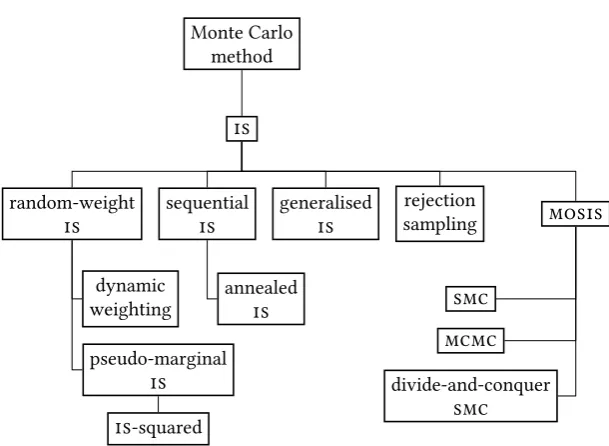
. One possible way of viewing the relationship between

(48)

1.5 Summary

Monte Carlo method

is

random-weight

is

dynamic weighting

pseudo-marginal

is is-squared

sequential

is

annealed

is

generalised

is samplingrejection mosis

smc mcmc

divide-and-conquer

[image:48.595.125.430.237.460.2]

smc

(49)

(50)

2 Sequential Monte Carlo Methods

2.1 Introduction

2.1.1 Motivation

In this chapter, we describe sequential Monte Carlo methods. Section 2.1

outlines a generic sequential Monte Carlo algorithm which admits essentially

all known sequential Monte Carlo algorithms as a special case. In Section 2.2,

we show that this generic algorithm can itself be viewed as a special case of

the marginalised one-sample importance sampling framework introduced in

Chapter 1 and thus as importance sampling. This was already established in

Andrieu et al. (2010) and extended to non-exchangeable resampling schemes

in Lee, Murray and Johansen (in prep.). We extend the latter construction

to also allow for biased resampling schemes. In Section 2.3, we interpret a

number of sequential Monte Carlo algorithms, such as the discrete particle

filter, as special cases of this framework. In Subsection 2.3.3 we generalise and

improve existing schemes for re-using all particles to approximate integrals.

Finally, in Section 2.4, we show that forward filtering–backward smoothing,

too, is a special case of importance sampling.

Sequential Monte Carlo (

smc

) methods are a class of Monte Carlo

schemes suitable for approximating a sequence of related measures. Dat-ing at least as far back as Stewart and McCarty Jr (1992), Gordon, Salmond and Smith (1993), Del Moral (1995),

smc

methods were originally de-veloped to approximate the optimal filtering problem in discrete-time target tracking applications, e.g. in non-linear or non-Gaussian(general state-space) hidden Markov models(

hmm

s) (sometimes calledstate-space models). In this particular setting, they are often called ‘particle filters’.

(51)

(Cérou, LeGland, Del Moral & Lezaud, 2005), for inference in continuous-time models (Fearnhead et al., 2010), for optimisation (Johansen, Doucet & Davy, 2008), for model selection (Peters, 2005; Jasra, Doucet, Stephens & Holmes, 2008; Yan Zhou, Johansen & Aston, 2013), and for approximately solving inverse problems (Kantas, Beskos & Jasra, 2014).

A tutorial-style introduction to the area can be found in Doucet and Johansen (2011). A book-length treatment of their application to

hmm

s can be found in Cappé et al. (2005). A comprehensive theoretical framework was developed in the monographs Del Moral (2004, 2013) – see also, Del Moral and Doucet (2014) for a gentle introduction to this framework in the case of finite state spaces.

Various kinds of

smc

algorithms have been developed, each tailored to individual problems. We detail some of these in Section 2.3. Essentially any such algorithm can be viewed as special cases of the generic

smc

al-gorithm presented in the next subsection. In turn, as shown in Section 2.2, the generic

smc

algorithm can itself be viewed as no more than a special case of themarginalised one-sample importance sampling(

mosis

) scheme

described in Chapter 1.

The basic idea of

smc

methods is as follows. Assume that we want to approximate (integrals with respect to) a family of positive finite measures

.Qt/t2T; usually,TDNT, forT 2 NorT DN. In this case, we can define

a sequence of extended measures.t/t2T, wheret 2M.X₁_Wt/, such that t admitsQt as a marginal. As described in Section 1.3 in the previous

chapter, working on such a product spaceX₁_W_t _WD

t_s_D₁Xs, which typically

includes all random variables generated over the course of the algorithm, is usually necessary to circumvent the calculation of intractable integrals related to the importance weights.

At Step t 1, the algorithm approximates t ₁, and thus Qt ₁, by

weighted samples. To obtain an approximation oft, and thusQt,

smc

methods can be thought of as extending and re-weighting an existing collection of sample points, often called ‘particles’.

2.1 Remark. To reduce the notational burden, we assume here that the number of particles generated at Stept,N_t 2 T, is deterministic. However, all developments in this chapter still hold if it was made a (non-degenerate)

random variable as, for instance, in Crisan et al. (1998), Jasra, Lee, Yau and

(52)

2.1 Introduction

2.1.2 Particles and Parent Indices

LetXt WDXt1WNt denote the collection ofNt particles which takes values

inXt WDXNt

t . These are generated at Stept of an

smc

algorithm targeting

a measuret 2M.X₁_Wt/, whereX₁Wt WD

t

sD1Xs. Thenth particle at Steps, Xn

t , will be considered as the offspring of theAnt ₁th particle generated at

Stept 1. We therefore callAn_t ₁thenth parent index sampled at Stept.

For simplicity, we collect the parent indices in vectors At ₁WDA1tWN1t

taking values inAt ₁ WDKNt

t ₁, whereKt WDNNt.

To simplify the notation, we collect all random variables generated by the

smc

algorithm at Stept in a vectorZt. That is, we writeZ₁ WDX₁

andZt WD .Ot ₁;At ₁;Xt/, fort > 1. These take values in the spaces Z₁ WD X₁ andZt WD Ot ₁ At ₁ Xt, for t > 1. Here, Ot ₁ is an

auxiliary variable taking values in some spaceOt ₁. It will parametrise

the proposal and resampling kernels and hence allow us to formalise adaptive resampling schemes, for instance.

After Stept 1, we have already sampledZ₁_Wt ₁based on which we have

constructed an approximation oft ₁given by the weighted empirical

measure

smc;N1Wt ₁

t ₁ WD Nt 1

X

nD1

wn_t ₁.Z₁Wt ₁/•_XBn1Wt 1jt 1 1Wt 1 :

Here, we have used the following notation.

Xb1Wt

1Wt D.X b₁

1 ; : : : ; Xtbt/denotes the particlepathortrajectory

associ-ated with some particle indicesb₁_Wt.

B₁n_W_t_j_t D.B₁n_j_t; : : : ; Bn_t_j_t/represents the particle indices formed by

tra-cing back the nth ancestral lineage at Step t (as determined by the

parent indicesA₁_Wt 1 D.A1; : : : ;At 1/), i.e.B_tn_j_t Dnand

B_sn_j_t DABsnC1jt

s ; fors < t.

wn_t ₁.z₁Wt ₁/2 Œ0;1/is a weight associated with thenth particle path

at Stept. As before, we use this terminology even though these ‘weights’

do not sum to 1, in general. The correspondingself-normalisedweights

(53)

At Stept, to obtain an approximation oft,

smc;N1Wt

t WD

Nt X

nD1

wn_t.Z₁Wt/•_XBn1Wtjt

1Wt ;

smc

algorithms sample additional particles, parent indices and potentially other auxiliary random variables, all collected in the ordered setZt, from

a particular stochastic kernel t 2 K₁.Z₁_Wt ₁;Zt/ defined below. The

extended set of samplesZ₁_Wt is then used to construct a new collection

of weights, .wn_t.z₁_Wt//n2Kt. In many cases, the computational cost of

sampling the additional random variables and of computing the new weights is constant int. This constant cost per step makes

smc

methods

particularly beneficial in settings in which sequences of measures need to be approximated under computational constraints, e.g. in real-time object-tracking applications.

The conditional distribution of the random variables generated at Stept

is then given by the stochastic kernel

t.z₁Wt ₁;dzt/WDSt ₁.z₁Wt ₁;dot ₁/Rt ₁..z₁Wt ₁; ot ₁/;dat ₁/