warwick.ac.uk/lib-publications
Original citation:
Bayvel, Polina, Maher, Robert, Xu, Tianhua, Liga, Gabriele, Shevchenko, Nikita A., Lavery,
Domaniç, Alvarado, Alex and Killey, Robert I.. (2016) Maximizing the optical network
capacity. Philosophical Transactions of the Royal Society A: Mathematical, Physical and
Engineering Sciences, 374 (2062). 20140440.
Permanent WRAP URL:
http://wrap.warwick.ac.uk/93957
Copyright and reuse:
The Warwick Research Archive Portal (WRAP) makes this work of researchers of the
University of Warwick available open access under the following conditions.
This article is made available under the Creative Commons Attribution 4.0 International
license (CC BY 4.0) and may be reused according to the conditions of the license. For more
details see:
http://creativecommons.org/licenses/by/4.0/
A note on versions:
The version presented in WRAP is the published version, or, version of record, and may be
cited as it appears here.
rsta.royalsocietypublishing.org
Research
Cite this article:Bayvel P, Maher R, Xu T, Liga G, Shevchenko NA, Lavery D, Alvarado A, Killey RI. 2016 Maximizing the optical network capacity.Phil. Trans. R. Soc. A374: 20140440. http://dx.doi.org/10.1098/rsta.2014.0440
Accepted: 14 December 2015
One contribution of 14 to a discussion meeting issue ‘Communication networks beyond the capacity crunch’.
Subject Areas:
optics, electrical engineering
Keywords:
optical fibre communications, optical nonlinearities, Kerr effect, channel modelling, signal processing, optical networks
Author for correspondence:
Polina Bayvel
e-mail:[email protected]
Maximizing the optical
network capacity
Polina Bayvel, Robert Maher, Tianhua Xu, Gabriele
Liga, Nikita A. Shevchenko, Domaniç Lavery,
Alex Alvarado and Robert I. Killey
Optical Networks Group, University College London,
Torrington Place, London WC1E 7JE, UK
TX,0000-0002-5510-841X; AA,0000-0002-2172-3051
Most of the digital data transmitted are carried by optical fibres, forming the great part of the national and international communication infrastructure. The information-carrying capacity of these networks has increased vastly over the past decades through the introduction of wavelength division multiplexing, advanced modulation formats, digital signal proces-sing and improved optical fibre and amplifier technology. These developments sparked the com-munication revolution and the growth of the Internet, and have created an illusion of infinite capacity being available. But as the volume of data continues to increase, is there a limit to the capacity of an optical fibre communication channel? The optical fibre channel is nonlinear, and the intensity-dependent Kerr nonlinearity limit has been suggested as a fundamental limit to optical fibre capacity. Current research is focused on whether this is the case, and on linear and nonlinear techniques, both optical and electronic, to understand, unlock and maximize the capacity of optical communications in the nonlinear regime. This paper describes some of them and discusses future prospects for success in the quest for capacity.
1. Introduction: optical fibre, the illusion of
infinite capacity and why more bandwidth
is needed
It is hard to imagine now that, since the introduction of the first optical fibre systems in the 1970s, pioneered in
2
rsta.r
oy
alsociet
ypublishing
.or
g
Ph
il.T
ran
s.R
.So
c.A
37
4
:2
0140440
...
the UK’s historic and heroic Standard Telecommunication Laboratories and BT Research Labs (or the Post Office as it was then), the achievable transmission rates have increased by some six orders of magnitude, with three orders of magnitude increase in achievable distances. Optical fibre now underpins the global communications infrastructure with state-of-the art laboratory
experiments achieving data rates in excess of 50 Tb s−1, using hundreds of wavelengths, over a
single fibre core. The commercial systems lag these achievements but are not far behind. For many years it has been thought and claimed that, for all practical purposes, optical fibres have infinite capacity which would never be exhausted. And yet, the development of optical fibre technology has almost become the ‘victim’ of its own success.
For the last 40 years, the network providers have continually argued, with each generation, that optical fibre capacity of that generation is sufficient and little more is necessary. However, the availability of high-capacity fibre has provided the impetus for the growth of telecommunication, fuelling the development and proliferation of data services unfathomed and unfathomable at the time of the first systems being installed. The growth of the digital economy and the extension of our lives online provide a powerful argument that the provision of high capacity and ubiquitous fibre connectivity will lead to new services, and history has shown that it is a mistake to consider past or even current usage of scarce resources as a reliable guide to future demands in this fast growing and competitive domain. Indeed, a number of recent economics studies have analysed productivity increases through availability of broadband digital services and have demonstrated that these lead to additional increases in per annum productivity by as much as 0.4%, where total productivity growth in most economies is about 1.5%. Using the current UK gross domestic
product of £1.7tr as an example, this would lead to an attributable gain of some £6.8bn [1].
It is hard to speculate about the future, but new services might include personalized genetic medicine for cancer or other diseases which requires transmission of DNA information with data requirements of some 1.5 GB per sequence. Treatments may require several sequences such that more than half a terabyte of data are transmitted, several times a day. Assisted ambient living and lifelong monitoring are also expected to result in significant data transmission demands, none of which can be satisfied with current capacity provisions. The ‘Internet of Things’, in which numerous consumer and sensor devices will also be connected to the Internet, has a projected number of 50 billion devices by 2020, and will add significant additional traffic to the network. Even without the addition of new services, current growth rates are greater than
20% per year with Cisco VNI forecasting [2] global public network traffic demands of some
130 exabytes (1018 bytes) per month in 2018—equivalent to 200 million DVDs. To put this
in context—-500 exabytes is equivalent to the content of the Internet in 2009 (by 2013 it had reached 4000 exabytes!). Furthermore, the proliferation of data centres and cloud services has been accompanied by machine-to-machine traffic—not included in forecasts for traffic growth, but likely to add significantly to future capacity requirements.
So just how much data can be transmitted over optical fibre? Reported ‘record’ results vary by the metrics used to measure the capacity and distances over which transmission is reported. For example, the highest total capacity in bits per second, on a single fibre core
is 102.3 Tbit s−1, transmitted over 240 km [3], using WDM DP-64QAM (wavelength division
multiplexed dual-polarization 64-ary quadrature amplitude modulation) and digital coherent
detection. Another metric is spectral efficiency (SE), measured in bit s−1Hz−1 (or bit/s)/Hz
and defined as the total capacity divided by the transmission bandwidth. The highest SE reported to date is 15.3 bit s−1Hz−1[4], corresponding to 66.6 Gbit s−1single carrier DP-2048QAM over a relatively short distance of 150 km. Yet another measure is highest capacity–distance
product over transoceanic distances. The current record for this metric is 52.2 Tbit s−1 over
10 230 km (534 Pbit s−1km) and 54 Tbit s−1over 9150 km (494 Pbit s−1km) at spectral efficiencies
of 5–6 bit s−1Hz−1, using 180/200 Gbit s−1 DP-16QAM channels [5]. Often the SE is specified
without reference to the bandwidth over which the transmission performance was investigated and, as we shall show later, it is much more challenging to achieve the same performance over a larger bandwidth. Yet another metric is the SE–distance product, with a record of
3
rsta.r
oy
alsociet
ypublishing
.or
g
Ph
il.T
ran
s.R
.So
c.A
37
4
:2
[image:4.493.66.431.43.189.2]0140440
...
100
NEC, 101.7 Tbit s
–1 [9]
NTT, 102.3 Tbit s
–1 [3]
OOK DP-OOK
DQPSK 128QAM DP-128QAM DP-512QAM DP-2048QAM
PSBT DPSK
DP-DQPSK
DP-8QAM
DP-16QAM
DP-64QAM
OFDM
15
10
5
0 80
60
capacity (Tbit s
–1
)
SE (bit s
–1 Hz –1)
40
20
0
1999 2001 2003 2005 2007 2009 2011 2013 2015 1999 2001 2003 2005 2007 2009 2011 2013 2015
NTT, 69.1 Tbit s–1 [10]
Tohoku Univ., 15.3 bit s–1 Hz–1 [4]
Tohoku Univ., 12.19 bit s–1 Hz–1 [16]
Tohoku Univ., 10 bit s–1 Hz–1 [17]
Tohoku Univ., 5 bit s–1 Hz–1 [18]
KDDI, 1.6 bit s–1 Hz–1 [19]
NTT, 1 bit s–1 Hz–1 [20]
NTT, 20.4 Tbit s–1 [12]
Alcatel, 3.65 Tbit s
–1 [15]
Alcatel, 6.3 Tbit s
–1 [14]
AT&T
, NEC, Corning, 32
Tbit s
–1
[11]
OFS, 6.4 Tbit s–1 [13]
(a) (b)
Figure 1.(a) Capacity and (b) SE growth demonstrated in state-of-the art laboratory and research experiments around the world. It should be noted that figures for SE are difficult to compare as experiments are performed over different bandwidths but the trend is interesting nonetheless [3,4,9–20].
The highest capacity per channel is 10.2 Tbit s−1 (1.28 TBd) [7], achieved using optical time
division multiplexing with DP-16QAM. Recent research on space-division multiplexing using
multi-core fibre technology has yielded the highest total capacity per optical fibre [8] of
2.15 Pbit s−1 over 31 km of 22-core single-mode fibre. The relentless growth in experimentally
achieved records is summarized infigure 1. It should be noted that, to make a fair comparison,
only the useful information bits should be considered, i.e. the overheads added for forward error correction (FEC), necessary to correct the bit errors introduced in noisy and nonlinearly distorted signals, should be excluded. We shall return to this point in later sections but care should be taken with the analysis of reported results which often describe raw bits without subdividing them into bits carrying useful data and the coding overheads.
One simple solution to the capacity exhaust problem might be to install (or ‘light up’) additional fibres. The reluctance by operators to do this is a question of cost—adding more
fibres, N, means that systems costs scale linearly withN, as they requireNtimes more inline
amplifiers, transceivers, power, and so on, resulting in a stagnating cost per bit transmitted. The growth in services and digital data traffic has been predicated on cost per bit going down which has now, within the current technology limits, asymptotically approached such low levels that further reductions appear challenging or even unrealizable. Something quite different must happen for cost per bit to continue on its path of reduction—such as dramatic capacity increases per system installed. This paper is intended to explain the needs and the challenges of increasing the amount of data which can be transmitted over optical fibres and the metrics used to measure them. The Kerr nonlinearity limit is explained, in the next section, together with a description of different techniques proposed to date to overcome it. One technique, namely multi-channel digital backpropagation (MC-DBP), is described in detail, from analytical (§3), numerical simulations (§4) and experimental perspectives (§5), over a range of modulation formats, and it is shown that it can lead to the doubling in the maximum transmission distance. The paper concludes on the prospects of future capacity increases, and discusses lower bounds as a function of fibre bandwidth, modulation formats and nonlinearity compensation, in §6.
2. Fibre capacity limits?
What limits the continued growth of achievable data rates in optical fibres? It was Claude
Shannon who first introduced the concept of channel capacityin his 1948 paper [21]. The most
4
rsta.r
oy
alsociet
ypublishing
.or
g
Ph
il.T
ran
s.R
.So
c.A
37
4
:2
0140440
...
transmission is possible (see more details in §3). Unfortunately, for most (if not all) channels, no closed-form expression for the channel capacity exists. Fortunately, many channels (such as copper wires and wireless channels) can be accurately modelled using an additive white Gaussian noise (AWGN) channel model, in which case, the channel capacity is the elegant equation
C=B·log2(1+SNR), (2.1)
whereBis the bandwidth and SNR is the signal-to-noise ratio of the channel.
Since its derivation, over 60 years ago, coding and information theorists have tried to approach this capacity limit with low-complexity coding schemes. For binary modulation, they have indeed
succeeded, with performance within fractions of a dB [22]. A good review of these efforts can be
found in [23].
The use of the information-theoretic capacity concept for the optical fibre channel dates back to the work of Splettet al.in 1993 [24]. However, it is only recently that this concept became popular in the optical fibre literature. This was prompted by the slowing in the dramatic capacity growth,
outlined above [25], which had become constrained due to the fact that the optical fibre channel is
nonlinear. The channel capacity analysis has turned out to be surprisingly difficult. A good review is given by Essiambre & Tkach [26].
The optical fibre channel is fundamentally nonlinear, which means that the refractive index of
the propagation mediumneffchanges in response to the strength of the square of the electric field
Eor optical intensityI,
neff=n0+n2I, (2.2)
wheren0andn2are the linear and nonlinear refractive indices, respectively; the normalized time
averaged electric fieldEis related to optical intensity as|E| =√P, wherePis the optical power in the fibre andI=P/AeffwithAeffthe effective area of the fibre. For silica,n0≈1.5 andn2≈3×
10−20m2W−1. After a transmission distanceL, the nonlinear optical Kerr effect will result in a phase shift, which, when added to the shift from linear propagation, results in a total phase shift, given by
ϕ=k0n0L+ϕNL, (2.3)
where k0=2π/λ0 is the free-space wavenumber, λ0 is the optical wavelength and ϕNL is a
nonlinear phase shift. This phase shift depends on the optical signal powerPas
ϕNL=γPL (2.4)
andγ is the fibre nonlinear coefficient, a measure of nonlinearity,
γ=k0n2
Aeff. (2.5)
Transmission of more data within a finite bandwidth requires greater optical power levels P,
which leads to the power-dependent nonlinear distortion of the transmitted data. This imposes a Kerr nonlinearity limit, sometimes referred to as the nonlinear Shannon limit. Strictly speaking, however, this limit is only a lower bound to the channel capacity, as it assumes that nonlinear interference is noise (whereas, as shown above, it is deterministic).
The propagation of the amplitude and phase of the electric fieldEis governed by the nonlinear
Schrödinger equation (NLSE)
∂E(z,t)
∂z +j
β2
2
∂2E(z,t)
∂t2 +
α
2E(z,t)=jγ|E(z,t)|
2E(z,t), (2.6)
wherezandtrepresent space and time, respectively. The NLSE in (2.6) captures the effects of Kerr
nonlinearity (via the nonlinear parameterγ), loss (via the attenuation parameterα) and chromatic
dispersion (via the group velocity dispersionβ2) in the fibre. Furthermore, amplified spontaneous
5
rsta.r
oy
alsociet
ypublishing
.or
g
Ph
il.T
ran
s.R
.So
c.A
37
4
:2
0140440
...
method, which iteratively and alternately solves the linear and nonlinear elements of the above equation. There are currently no closed-form expressions exactly describing fibre propagation for arbitrary input signal shapes.
Channel capacity calculations require a channel model (also known as channel law). The
difficulty in quantifying the capacity of the nonlinear optical fibre channel is that no explicit (and simple) channel model exists. As mentioned above, the NLSE is a precise model; however, it is not explicit, i.e. the output of the channel is not expressed as a simple function of the input. The nonlinear fibre channel also introduces memory and the signal also interacts nonlinearly with the ASE noise. All these effects present a considerable challenge to the definition of the nonlinear channel model, a source of some debate of recent years, and a focus of much recent research activity, as explained by Agrellet al. [27].
There have been numerous proposals to overcome the Kerr nonlinearity limit or at least to mitigate the impact of nonlinearities. Some of the techniques are discussed in the following subsections.
(a) Digital backpropagation
Digital backpropagation (DBP) is a fibre nonlinearity mitigation technique which can be applied both to a single channel and to a multi-channel (WDM) system. In the former case to compensate for self-phase modulation (SPM)—the nonlinear interference of a channel induced by its own electric field; in the latter case to mitigate for nonlinear distortions from both SPM and multi-channel nonlinearities (cross-phase modulation (XPM) and four-wave mixing (FWM)), caused by the electric field from adjacent WDM channels. This is done by simultaneously receiving and processing multiple optical channels using a high-bandwidth receiver.
In DBP, the NLSE in (2.6) is solved, in its inverse form, in the digital domain, by changing the sign of all the propagation parameters, allowing for the Kerr nonlinearity to be compensated, either fully or partially, i.e.
⎧ ⎪ ⎨ ⎪ ⎩
α→ −α β2→ −β2
γ→ −γ
⎫ ⎪ ⎬ ⎪
⎭⇒
∂E(z,t)
∂z −j
β2
2
∂2E(z,t)
∂t2 −
α
2E(z,t)= −jγ|E(z,t)|
2E(z,t). (2.7)
DBP aims at reconstructing the transmitted signal and is typically applied at the receiver. However, DBP can also be applied at the transmitter or split between the two. In all cases, however, complete reconstruction of the signal is not possible because of nonlinear mixing between the signal and the ASE noise as well as other stochastic effects such as polarization
mode dispersion [28–30]. Applying DBP at the transmitter (sometimes termed as nonlinear
pre-distortion or transmitter-based pre-distortion) or at the receiver gives approximately the same gains (determined by the accumulation of noise from the amplifier in the link) with one
fewer amplifier noise contribution in the transmitter-based DBP case [31,32]. In the case of long
transmission distances (greater than 10 spans), this difference is insignificant. In fact, it is clear that to reduce the contribution of noise, DBP should be split in the ratio of 50% : 50% between the transmitter and receiver. However, the greatest increase in the effectiveness of DBP can be achieved by reverse propagation of multiple channels, enabling the compensation of not only
SPM but also inter-channel nonlinearities (XPM) [33]. The gains offered by DBP are discussed in
detail in §§3, 4 and 5.
(b) Optical phase conjugation
6
rsta.r
oy
alsociet
ypublishing
.or
g
Ph
il.T
ran
s.R
.So
c.A
37
4
:2
0140440
...
profile is required, to ensure that distortion caused in the first half of the link is accurately
reversed by that in the second half (see [34,35]). Recent achievements include dual-band optical
phase conjugation of an optical superchannel using 75 km spans of standard single-mode
fibre [35], where it was possible to substantially eliminate inter-channel nonlinear penalties;
this nonlinearity compensation resulted in approximately 50% increase in transmission reach for
six simultaneously transmitted 400 Gbit s−1DP-16QAM superchannels, a record total bit rate of
2.4 Tbit s−1using one dual-band OPC. In future, it may be possible to combine OPC with DBP for
additional performance gains.
(c) Nonlinearity-tailored detection
DBP is a zero-forcing equalization technique, and thus can be outperformed under certain circumstances by improved detection techniques that account for noise, nonlinearity and the memory of the channel. Given a noisy observation from the channel, optimal detection techniques minimize the error probability based on the noise distribution. For a multispan link, a closed form
for this distribution is not available, and thus approximated solutions have been proposed [36].
Additionally, unlike the single span case, the interaction between signal and ASE noise limits the SNR at the receiver. As a result of this, the uncoded bit-error rate (BER) does not monotonically decrease as a function of the transmit power, even with improved detection. The problem of optimal detection of signals transmitted through a nonlinear channel with memory is theoretically important as it represents a preliminary step in the design of optimal receivers for more complex channel models. Recent promising results have been reported showing optimum detection for the single span fibre channel with a near-optimum detector in the presence of both nonlinear
distortions and memory [37]. Despite the significant nonlinearity at the high values of transmitted
powers used, it was shown that uncoded BER can be made arbitrarily low in this regime when the detector is tailored to the nonlinear properties of the channel, effectively acting as a ‘nonlinear matched filter’. More work remains to be done in this promising area.
(d) Nonlinear Fourier transform and eigenvalue communications
This approach is a transmission and signal processing technique that makes positive use of the
nonlinear properties of fibre channels. The NLSE is a member of a unique class of integrable
nonlinear equations that can be solved via the so-called inverse scattering transform method [38].
This is an extension of the linear Fourier transform into nonlinear systems and is known as the
nonlinear Fourier transform (NFT) [39–41]. The principle of the NFT involves the transformation
of the effects of both nonlinearity and dispersion to a simple phase rotation of continuous nonlinear spectral data that play the role of a Fourier spectrum for nonlinear problems. The
pioneering work of Hasegawa & Nyu [42] used discrete eigenvalues to encode and transmit
information, as these are unaffected by dispersion and nonlinearity. There is currently much focus on this approach as it allows one to make positive use of the nonlinear properties of the fibre channel, since in integrable nonlinear channels, there are nonlinear normal modes that also propagate without any resulting nonlinear cross-talk; effectively in a linear manner. The conversion from the space–time domain into the nonlinear spectral domain and back is performed through the forward NFT and inverse NFT, respectively.
Alternative approaches to increasing capacity include a range of techniques which are in different stages of development such as coding tailored to the nonlinear channel, multi-channel all-optical and electronic regenerators or noise squeezing, wideband optical amplifiers— capable of taking advantage of the entire low-loss fibre bandwidth of 400 nm (1200–1600 nm), approximately 50 THz, rather than the limit imposed by the EDFAs of approximately 40 nm—
and the use of negative n2 metamaterials which would allow for all-optical nonlinearity
compensation.
7
rsta.r
oy
alsociet
ypublishing
.or
g
Ph
il.T
ran
s.R
.So
c.A
37
4
:2
0140440
...
3. Estimating fibre capacity
(a) Channel capacity and mutual information
The channel capacity can be defined for a continuous-time input continuous-time output channel, which is modelled for example via the NLSE in (2.6). However, the channel capacity is more
commonly defined between thediscrete-timeinput and output constellation symbols, i.e. when
certain parts in the transmitter and receiver have been fixed (e.g. filtering, up/down-conversion, modulators, digital-to-analogue and analogue-to-digital convertors (ADCs)). For a detailed comparison between these two cases, see the paper by Agrellet al. [27].
The relationship between the input and output symbols is random, and thus it is modelled
using a conditional probability density function (PDF) pY|X(y|x), where Xand Y are random
vectors, both of lengthn, representing the transmitted and received symbols. The channel capacity
is then defined as
Cmem lim
n→∞maxpX(x)
1
nI(X;Y). (3.1)
In (3.1), the optimization is over all input distributionspX(x) that satisfy a power constraint and
I(X;Y) is the mutual information (MI) between the random vectorsXandY. MI describes the
information thatX andY share. MI (measured in bits or bits s−1Hz−1—by analogy with SE)
is the reduction of uncertainty inXthat we get from the knowledge ofY and vice versa. The
channel capacity definition in (3.1) is general in the sense that it considers possible memory in the channel, and thus random vectors are considered. On the other hand, the expression in (3.1) is mathematically hard to analyse. Nevertheless, this expression was used to evaluate (numerically) the capacity of a heuristic channel model for dispersive fibre-optic links with finite memory in [43].
If the channel memory is discarded and the transmitted symbols are independent and
identically distributed according to pX(x), a lower bound on the capacity can be found. In
particular, if anaveragePDFpY|X(y|x) is considered, we have Cmem≥max
pX(x)
I(X;Y), (3.2)
where the MI is defined as
I(X;Y)E log2pY|X(Y|X)
pY(Y)
(3.3)
andE[·] is the expectation operator.
If no maximization is performed in (3.3), yet another lower bound is obtained. This is the case when the constellation symbols are drawn with the same probability from a set of discrete constellation points (such as 16QAM or 64QAM), as usually done in practice. Mathematically, if
we denote the transmitted QAM symbols byXqam, we obtain the following inequalities:
Cmem≥max
pX(x)
I(X;Y)≥I(Xqam;Y). (3.4)
The expression in (3.4) simply shows that when the MI between the transmitted and received
symbolsI(Xqam; Y) is considered, only a lower bound on the capacity is obtained.
(b) Calculating the signal-to-noise ratio in nonlinear fibres
8
rsta.r
oy
alsociet
ypublishing
.or
g
Ph
il.T
ran
s.R
.So
c.A
37
4
:2
0140440
...
regime is still a much-debated open question, as it is based on the perturbation model approach to solving the NLSE (or other simplifying approximations). This so-called Gaussian noise model
of nonlinear interference (GN-model), also predicts that the SNR tends to zero at high power levels
which gives the incorrect impression of a channel capacity equal to zero in the highly nonlinear
regime. In view of (3.4), however, this only means that alower boundgiven by the GN-model tends
to zero, and not the channel capacity. Nevertheless, the GN-model is a convenient approximation and, if used carefully, can provide valuable insights. In particular, the SNR given by the GN-model can be used to evaluate theQ2factor or the MI in (3.3).
According to the GN-model, and under the assumption of incoherent accumulation of
nonlinearity, the SNR in an optical communication system can be expressed as [28,44]
SNR≈ P
PN+PS–S+PS–N, (3.5)
wherePis the optical signal power,PNis the total ASE noise in the transmission system,PS–Sis
the total nonlinear signal–signal interaction,PS–Nis the total nonlinear signal–noise interaction
and we have
PN=Nspan·PASE, (3.6)
PS–S=Nspan·ηP3 (3.7)
and PS–N=3ξηP2PASE, (3.8)
wherePASEis the ASE noise power from one EDFA,Nspanis the number of fibre spans,ηis the
nonlinear distortion coefficient according to the GN model andξ=Nspan(Nspan−1)/2 is a factor
depending on the number of spans. The ASE noise in the EDFA can be described as
PASE=1
2Np(GEDFA−1)Fn·hν·B, (3.9)
whereNpis the number of polarization states,GEDFAis the gain of the EDFA,Fnis the EDFA noise
figure,his Planck’s constant,νis the central frequency of the optical carrier andBrepresents the
optical bandwidth.
For dual-polarization EDFA amplification, and Nyquist-spaced WDM transmission systems,
the nonlinear distortion coefficientηcan be approximated using the following expression [44]:
η≈ 8γ2Leff
27π|β2|R2S
asinh
π2
2 |β2|Leff·B
2
, (3.10)
whereLeffis the fibre effective length andRSis the symbol rate of the signal.
It should be noted that a source of debate relates to the form of the SNR expression in (3.5), where the noise is power dependent and the signal and noise cannot be separated, nor fully mitigated! This means that the SNR changes its physical meaning with power which has motivated researchers to seek a more accurate channel model to describe the nonlinear channel. This remains an active and dynamic research area.
(c) Capacity lower bound calculations
The channel capacity of the nonlinear optical fibre channel (see Cmem in §3a) can be lower
bounded using the expression for channel capacity for the memoryless AWGN channel in equation (2.1):
C=2B·log2(1+SNR), (3.11)
9
rsta.r
oy
alsociet
ypublishing
.or
g
Ph
il.T
ran
s.R
.So
c.A
37
4
:2
0140440
...
For a linear AWGN channel, the SNR is calculated from (3.5) and (3.6) as
SNR= P
PN= P
NspanPASE (3.12)
and the resulting lower bound in (3.11) becomes the actual channel capacity.
In the case of the digital signal processing (DSP) following coherent detection performing electronic dispersion compensation (EDC) only, nonlinear signal–signal interaction (much larger than signal–noise interaction in equation (3.5), which can therefore be neglected in this case) is included in the noise term, in addition to ASE, so that the SNR is calculated as
SNR≈ P
PN+PS–S ≈
P
Nspan(PASE+ηP3). (3.13)
In the case of full-bandwidth DBP being applied as part of the receiver- or transmitter-based DSP, all nonlinear signal–signal interactions (including intra- and inter-channel nonlinearities) are removed, and only the signal–noise nonlinear interference is included in the noise term (in addition to ASE). The SNR is calculated using equation (3.5), as
SNR≈ P
PN+PS–N≈
P
NspanPASE+3ξηP2PASE. (3.14)
These expressions are applied to a variety of system simulations and experiments to test their validity in §4 and for capacity lower bound estimates in §6.
4. Numerical simulations of wavelength division multiplexing superchannel
DP-64QAM transmission
As previously mentioned, in this paper, we focus on one of the many possible techniques to overcome the Kerr nonlinearity limit, specifically that of MC-DBP, illustrating its performance through numerical simulations, experiments and capacity estimates. In this section, numerical simulations of this technique are described. These are of a Nyquist-spaced 9-channel 32 Gbaud
DP-64QAM WDM superchannel system, with a total raw data rate of 3.456 Tbit s−1. MC-DBP
with 64QAM [45] is an advance on the previously reported results [33] showing doubling in
achievable transmission distance. The achievable transmission distance of this superchannel system is evaluated both numerically, using the split-step Fourier algorithm, and analytically, using the perturbation-based GN-model, described in §3.
(a) Simulation set-up
The set-up of the 9-channel 32 Gbaud per subchannel DP-64QAM superchannel transmission
system is schematically illustrated in figure 2, and all numerical simulations were carried
out based on the split-step Fourier algorithm solving the NLSE with a digital resolution of 32 Sa/symbol. In the transmitter, an optical frequency comb generator was applied to generate the nine phase-locked 32 GHz-spaced optical carriers for the subchannels (centred at 1550 nm). Digital-to-analogue convertors (DACs) with a resolution of 16 bit (to ensure no back-to-back implementation penalty) and root-raised-cosine (RRC) filters with a roll-off of 0.1% were used for the Nyquist-pulse shaping. The transmitted symbol sequences were decorrelated with a delay of 256 symbols using a cyclical time shift to emulate the independent data transmission in each subchannel and the sequences in each polarization were also decorrelated with a delay of half the sequence length. The standard single-mode fibre (SSMF) was simulated based on the split-step Fourier method with a split-step size of 0.1 km, and the detailed system parameters were: span length of 80 km, α=0.2 dB km−1, β2= −21.7 ps2km−1 andγ=1.2 W−1km−1. Negligible fibre
PMD was assumed. The noise figure of the EDFA was set toFn=4.5 dB. At the receiver, the
10
rsta.r
oy
alsociet
ypublishing
.or
g
Ph
il.T
ran
s.R
.So
c.A
37
4
:2
0140440
...
PRBS
DAC
NPS
I-Q modulator
laser
comb I-Q modulator
delay
booster EDFA
LO 80 km SSMF
EDFA ×N
–10
–20
po
wer (dB)
–30
–40
–50
–60
–70
–200 –150 –100
–4 –3 –2 –1 0 1 2 3 4
–50 0
relative frequency (GHz)
50 100 150 200 PBS
PBS
coherent Rx
ADC
RRC f
ilter
EDC/DBP
do
wn sample
matched f
ilter
equalization
CPE
BER/FEC/MI
PBC
(a) (b)
Figure 2.(a) Schematic of 9-channel DP-64QAM superchannel transmission system using the EDC or MC-DBP and (b) simulated transmission spectrum and the schematic of backpropagated bandwidth in the 9-channel DP-64QAM superchannel transmission system, where the frequency 0 Hz refers to the central frequency of the optical carrier (wavelength of 1550 nm). (PBS, polarization beam splitter; PBC, polarization beam combiner; NPS, Nyquist pulse shaping).
and sampled at 32 Sa/symbol, without any bandwidth limitation, which allowed an ideal and synchronous detection of all the in-phase and quadrature signal components over the whole superchannel bandwidth. The DSP modules included a RRC filter for selecting the MC-DBP bandwidth, followed by MC-DBP (or linear EDC), down-sampling (to 2 Sa/symbol), matched filtering, multiple modulus algorithm equalization, ideal carrier phase estimation (CPE), symbol de-mapping and BER estimation. The simulated spectrum of the 9-channel DP-64QAM coherent
transmission system is shown infigure 2b, where the number represents the subchannel index
within the entire superchannel.
The EDC was realized using a frequency domain equalizer [46], and MC-DBP algorithm
was implemented using the reverse split-step Fourier method applied to the signal nonlinear propagation based on the Manakov equation (2.6) with a 0.5 split ratio for the chromatic
dispersion compensation [30,47]. An ideal RRC filter was applied to select the desired
backpropagated bandwidth for the MC-DBP, and also to reject the unwanted out-of-band ASE noise. The backpropagated bandwidth was 32 GHz for the single-channel DBP, increasing to 288 GHz for 9-channel (full-bandwidth) DBP. The sampling rate was 32 Sa/symbol both in the EDC and the MC-DBP operations. A matched filter was used to select the subchannel of interest and to optimize the SNR of the processed signal. The multiple modulus algorithm with 21 taps was used for the polarization equalization and residual linear impairment equalization. The CPE was realized using ideal phase estimation, assuming there is no phase noise in the Tx and LO laser. Finally, symbol de-mapping and BER estimation were carried out to assess the transmission
performance of the measured subchannel based on 218bits, with a pseudo-random bit sequence
pattern length of 215−1.
(b) Performance of multi-channel digital backpropagation in superchannel transmission
In all simulations, the MC-DBP algorithm was run with 800 steps per span, with a nonlinear
coefficient of γDBP=1.2 W−1km−1. The performance of the transmission system with the
MC-DBP algorithm applied at the receiver was investigated for the case in which the linewidths of both the transmitter and the LO lasers were set to 0 Hz to remove the influence from phase noise. The achievable transmission distance for different launch powers for the central subchannel
(with channel index 0 infigure 2b) in the 9-channel DP-64QAM Nyquist transmission system
was calculated and is shown infigure 3. The BER threshold was set to 1.5×10⁻² (Q2 factor
of approx. 6.7 dB), corresponding to a 20% overhead hard-decision FEC threshold, which is
assumed to correct the BER to below 10−15 [48]. These results were obtained using either EDC
11
rsta.r
oy
alsociet
ypublishing
.or
g
Ph
il.T
ran
s.R
.So
c.A
37
4
:2
[image:12.493.82.411.42.195.2]0140440
...
2000 1500 1200 880
500
transmission distance (km) 160
12 10 8 6
GN-model EDC only 1-channel DBP 3-channel DBP 5-channel DBP 7-channel DBP 9-channel DBP polynomial fit
4 2
optical launch po
wer (dBm)
0 –2 –4 –6 –8 –10 –12
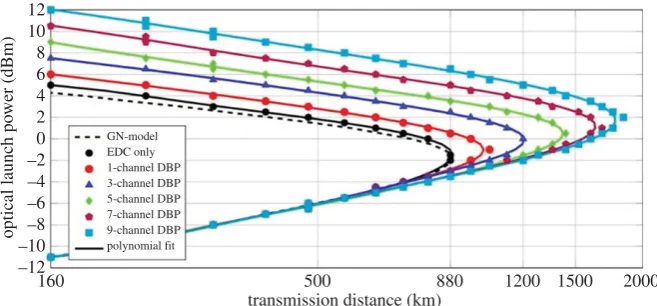
Figure 3.Maximum transmission distance as a function of different optical launch powers at a pre-FEC BER of 1.5×10⁻²in the 9-channel DP-64QAM superchannel transmission system using EDC and MC-DBP. The markers are the simulation data, and the solid line is the 5th order polynomial fit. The approximation obtained used the GN-model is also shown for EDC (dashed line).
can be seen that when EDC only is applied, the maximum transmission distance which can be
achieved is 880 km (11 SSMF spans) at the optimum launch power (−2 dBm). Single-channel
DBP can give an improvement of approximately 18% in the transmission distance (1040 km at
launch power of−1 dBm), whilst when all 9 channels are simultaneously detected and the entire
spectrum is digitally backpropagated to undo the nonlinearities, an improvement of over 109% in the transmission distance (1840 km at a launch power of 2 dBm) is obtained. The improved performance in the achievable superchannel transmission system can be seen with each increment in the MC-DBP bandwidth. In addition, the analytical prediction of the transmission performance
was also carried out using the perturbation theory-based GN model (of §3) [44,49], with good
agreement between the analytical prediction and the simulated reach curve with EDC.
The performance of the MC-DBP in the Nyquist-spaced 9-channel DP-64QAM superchannel
transmission system was also investigated in terms of Q2 factor for different optical launch
powers, as shown infigure 4. The transmission distance considered was the maximum achievable
distance—880 km (11 SSMF spans)—for the system using EDC only. All the Q2 factors are
converted directly from the measured BER values. It can be seen from figure 4 that the
performance of the MC-DBP in the superchannel transmission system improves with the
increment of the backpropagated bandwidth. The best achievable Q2 factor with EDC only
is approximately 6.7 dB at an optimum launch power of −2 dBm. When the single-channel
DBP is employed for SPM compensation, the best achievable Q2 factor was improved to
approximately 7.2 dB at an optimum launch power of −1 dBm. When the 9-channel
(full-bandwidth) DBP is applied over the whole superchannel for compensating the SPM, the XPM
and the FWM simultaneously, the best achievableQ2factor is improved to approximately 9.8 dB
at the optimum launch power of 2 dBm. The Q2 factor gain of the 9-channel (full-bandwidth)
DBP is approximately 3.1 dB compared with the EDC only case, and is approximately 2.6 dB compared with conventional single-channel DBP case. This investigation on the operation and the optimization of the MC-DBP indicates the optimal operation of the full-bandwidth DBP and a benchmark for the evaluation of the 9-channel DP-64QAM Nyquist superchannel transmission system.
(c) Digital backpropagation optimization and complexity
12
rsta.r
oy
alsociet
ypublishing
.or
g
Ph
il.T
ran
s.R
.So
c.A
37
4
:2
0140440
...
10
9
8
7
6
5
4
3
–8 –6 –4 –2 0
optical launch power (dBm) HD-FEC threshold
Q
2 f
actor (dB)
2 4 6 8
EDC only 1-channel DBP 3-channel DBP 5-channel DBP 7-channel DBP 9-channel DBP
Figure 4.Q2factor at 880 km (11 SSMF spans) in the 9-channel DP-64QAM transmission system using the MC-DBP over different
backpropagated bandwidths.
over all backpropagated subchannels, since all the information of the nonlinear interference in the involved subchannels is required for the MC-DBP to cancel both the intra-channel and the inter-channel nonlinearities. For EDC, it is only a requirement to apply the filtering over the bandwidth of the channel itself.
All the above numerical simulations have been implemented for a 9-channel 32 Gbaud Nyquist-spaced DP-64QAM optical transmission system. The findings can also be qualitatively applied to transmission systems using different modulation formats and different numbers of WDM subchannels. In addition to MC-DBP, as noted in the introduction, mid-span OPC is also a promising approach to compensate the fibre nonlinearities over multi-channel WDM transmission systems, where the phase conjugation of the transmitted signal is employed to generate, over the course of the second half of the transmission link, an opposite nonlinear phase shift for compensating the nonlinear effects generated in the first half of the transmission link [50,51].
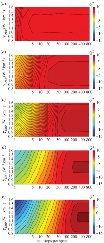
It is interesting to explore the efficacy of the MC-DBP algorithm. For simplicity, the linewidths of both the transmitter and the LO lasers can be set to 0 Hz for this analysis. The operation of the MC-DBP can then be investigated for different backpropagated bandwidths in terms of the
number of steps per fibre span and nonlinear coefficient parameter γDBP. We illustrate this for
the transmission distance of 880 km (11 SSMF spans), as before. The optimum launch power was always selected to achieve the lowest BER in the central subchannel for the particular
MC-DBP bandwidth used, as shown infigure 5. It can be seen that for the nonlinear coefficient of
γDBP=1.2 W−1km−1, in single-channel DBP (32 GHz), the minimum number of steps per span
is approximately 4, increasing to 300 in 9-channel (full-bandwidth) DBP. It is found that a good agreement between the minimum number of steps per span and the quadratic polynomial fit can be achieved.
There has been much discussion about the complexity of MC-DBP, which is indeed very
high in comparison with EDC [30]—possibly too high for it to become practical in the near
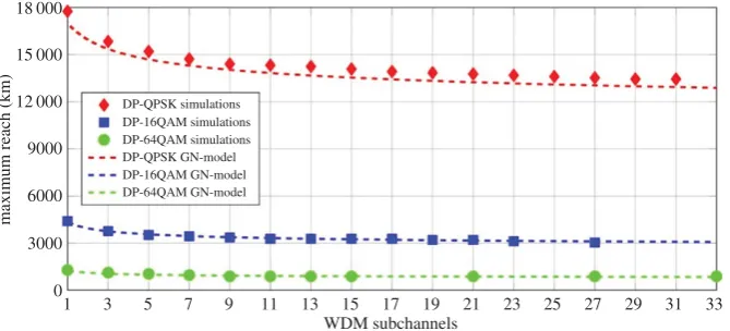
future for large bandwidth systems. However, simulations of achievable transmission distance using both simulations and the GN-model (albeit at the optimum power, and thus not in a very highly nonlinear regime) show that, for a given channel spacing or SE, although achievable reach
reduces with bandwidth, as shown infigure 6(reach versus number of channels for different
13
rsta.r
oy
alsociet
ypublishing
.or
g
Ph
il.T
ran
s.R
.So
c.A
37
4
:2
0140440
...1.6 Q 10
2 5 0 –5 –10 800 400 200 100 50 20 10 5 1 –15 gDBP (W –1 km
–1) 1.5 1.4 1.3 1.2 1.1 1.0 0.9 0.8
1.6 Q 10
2 5 0 –5 –10 800 400 200 100 50 20 10 5 1 –15 gDBP (W –1 km
–1) 1.5 1.4 1.3 1.2 1.1 1.0 0.9 0.8
1.6 Q 10
2 5 0 –5 –10 800 400 200 100 50 20 10 5 1 –15 gDBP (W –1 km
–1) 1.5 1.4 1.3 1.2 1.1 1.0 0.9 0.8
1.6 Q 10
2 5 0 –5 –10 800 400 200 100 50 20 10 5 1 –15 gDBP (W –1 km –1 ) 1.5 1.4 1.3 1.2 1.1 1.0 0.9 0.8
1.6 Q 10
2 5 0 –5 –10 800 400 200 100 50
no. steps per span10 20
5 1 –15 gDBP (W –1 km
–1) 1.5 1.4 1.3 1.2 1.1 1.0 0.9 0.8
(a)
(b)
(c)
(d)
(e)
Figure 5.Optimization of MC-DBP for different numbers of backpropagated subchannels:Q2factor as a function of the nonlinear coefficient and the number of steps per span used in the DBP algorithm. (a) 1-channel DBP, (b) 3-channel DBP, (c) 5-channel DBP, (d) 7-channel DBP and (e) 9-channel DBP.
for the DP-64QAM case, only approximately 5 channels need to be backpropagated, despite a much greater number of channels transmitted. This small number of channels accounts for most of the nonlinear interaction and resultant distortion with channels further away contributing significantly less distortion. Digital back propagation is fast becoming a practical reality with
first DSP chips currently being tested,1and the significant progress made in this area is likely to
continue.
1seehttp://www.ntt-electronics.com/en/news/2015/9/200g-high-performance-dsp.htmlfor a recent press release on the
14
rsta.r
oy
alsociet
ypublishing
.or
g
Ph
il.T
ran
s.R
.So
c.A
37
4
:2
[image:15.493.82.417.43.195.2]0140440
...
1 18 000
15 000
maximum reach (km)
12 000 DP-QPSK simulations
DP-16QAM simulations DP-64QAM simulations DP-QPSK GN-model DP-16QAM GN-model DP-64QAM GN-model
9000
6000
3000
0
3 5 7 9 11 13 15 17 19
WDM subchannels
21 23 25 27 29 31 33
Figure 6.Maximum reach versus number of channels for different modulation formats (at a pre-FEC BER of 1.5×10⁻²).
Comparison of results from numerical simulations and analytical calculations using the GN-model.
5. Experimental transmission of Nyquist-spaced DP-64QAM superchannel and
multi-channel digital backpropagation
Having investigated transmission by numerical simulations in the previous section, we now focus on experimental demonstrations of multi-channel transmission experiments and the effectiveness of practically implemented MC-DBP. MC-DBP was previously demonstrated experimentally
using a spectrally sliced coherent receiver to achieve aQ2 factor gain of approximately 1 dB by
backpropagating a 5-channel 30 GBd DP-16QAM superchannel [52]. A single coherent
super-receiver, which simultaneously receives and demodulates multiple optical subchannels, was
demonstrated by Tanimuraet al.[53] to backpropagate a 4-channel 28 GBd optical superchannel
and an enhanced Q2 factor margin was demonstrated at a fixed distance of 1000 km. A
single digital coherent receiver was also used to simultaneously receive a 7-subchannel 10 GBd subchannel Nyquist-spaced DP-16QAM superchannel and MC-DBP was subsequently employed
to increase the maximum reach of the transmission system by 85%, from 3190 to 5890 km [33].
Seven subchannels were used in the experiment described in this section, as in [54] (rather
than the nine considered in the simulations described in §4) so that the entire superchannel could be detected simultaneously within the super-receiver analogue electrical bandwidth of 63 GHz, as described below. The entire DP-64QAM signal with seven 10 GBd subchannels was simultaneously received using a digital coherent super-receiver and the performance of each subchannel was analysed after transmission over 1280 km of SSMF, both with and without MC-DBP. The role played by coding for adaptive FEC is also described.
(a) Transmission experimental set-up
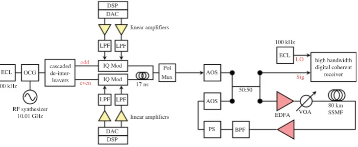
The 7-subchannel 10 GBd DP-64QAM superchannel transmission system is shown infigure 7.
15
rsta.r
oy
alsociet
ypublishing
.or
g
Ph
il.T
ran
s.R
.So
c.A
37
4
:2
[image:16.493.66.432.42.193.2]0140440
...
DSP DAC
LPF
OCG ECL
100 kHz
RF synthesizer 10.01 GHz
odd
cascaded
de-inter-leavers even
LPF
LPF LPF
DAC DSP
IQ Mod Pol
Mux AOS
50:50
LO
ECL 100 kHz
Sig
EDFA VOA 80 km SSMF high bandwidth digital coherent
receiver 17 ns
AOS
PS BPF
IQ Mod
linear amplifiers
linear amplifiers
Figure 7.DP-64QAM superchannel experimental set-up. AOS, acousto-optic switch; PS, polarization scrambler; VOA, variable optical attenuator; BPF, band pass filter.
were independently modulated using two complex IQ modulators, which were subsequently decorrelated before being combined and polarization multiplexed to form a Nyquist-spaced DP-64QAM superchannel. A conventional recirculating loop configuration was used for the emulation of long-haul transmission and included a single 80 km span of SSMF. Finally, the polarization diverse coherent receiver had an electrical bandwidth of 70 GHz and used a second 100 kHz external cavity laser as an LO for the coherent detection process. The emission frequency of the LO was set to coincide with the central subchannel of the DP-64QAM superchannel and the received signals were captured using a 160 GSa/symbol real-time sampling oscilloscope with 63 GHz analogue electrical bandwidth. The key receiver DSP blocks were identical to that illustrated infigure 2a.
Three figures of merit were employed to measure the performance of the superchannel transmission system. These include the BER calculated before FEC, the BER calculated after FEC and the MI. The combination of multi-level modulation, such as the 64QAM format used in this work, and FEC is known as coded modulation (CM). In a CM-based optical communications system, the transmitter passes information bits into a binary encoder, which adds redundancy that is used for error correction at the receiver and operates at a code rateRSD=Nb/Nc, whereNbis the
number of information bits andNcis the number of coded bits. The coded bits are mapped to a set
of discrete constellation points (64 in this case) using a memoryless mapper and are subsequently transmitted over the optical channel. The receiver consists of a memoryless demapper and a FEC decoder. A soft decision FEC (SD-FEC) decoder was used in this experiment to correct bit errors at the receiver (described in detail in [33]), albeit for a reduction in SE due the added redundancy, which is scaled by the required code rate. The pre-FEC BER was calculated before the SD-FEC decoder by passing the received symbols through a hard decision (HD) de-mapper, while the post-FEC BER is calculated by comparing both the encoded and decoded bits, which are obtained
at the output of the SD-FEC implementation [54] The MI between the transmitted and received
symbols is a key quantity in information theory, as it represents the largest achievable information rate for any CM-based system. It is calculated between the transmitted and received symbols
using Monte Carlo integration and is described in detail in the methods section of [34]. The MI
is normalized by dividing bym, and thus provides the largest code rate,R, that can be used to
achieve an arbitrarily low BER for a given CM system. For a practical FEC implementation, the
total code rate of the error correcting scheme must be less than or equal toR. This code rate can
be easily converted to a FEC percentage overhead through OH %=[(1/R)−1]×100.
In this experimental demonstration, a low-density parity-check-based SD-FEC scheme was
implemented offline in Matlab and is again detailed in the methods section of [34]. An outer HD
staircase code (SCC) that had a code rateRHD=16/17 was assumed. This outer HD-FEC code
16
rsta.r
oy
alsociet
ypublishing
.or
g
Ph
il.T
ran
s.R
.So
c.A
37
4
:2
0140440
...
post-FEC BER, measured at the output of the SD-FEC implementation, was below the threshold
for the outer concatenated SCC, then a BER of 10−15 was assumed to have been achieved. The
concatenated code rateRSDRHD must be less than or equal toR, as calculated by normalizing
the MI.
(b) Pre- and post-forward error correction bit-error rate performance
The pre- and post-FEC BER as a function of launch power for the central subchannel is displayed infigure 8. After 640 km transmission over SSMF and with EDC only, the pre-FEC BER reduced
linearly as the launch power increased from −18 dBm to −8 dBm, as seen infigure 8a. The
minimum BER was achieved at an optimum launch power of −6.5 dBm, after which the
pre-FEC BER began to increase with higher launch power due to signal distortions arising from fibre nonlinearity. The corresponding post-FEC BER, measured at the output of the SD-FEC decoder
with RSD=5/6 (corresponding to an overhead (OH) of 20%), is also shown infigure 8a. This
reduced the BER below the threshold for the outer HD SCC and also provided a launch power margin of approximately 6 dB (at the HD-FEC threshold). When the transmission distance was
increased to 1280 km (figure 8b), the pre-FEC BER at the optimum launch power increased from
2.6×10⁻²to 5.6×10⁻². Therefore, a SD-FEC code withR
SD=3/4 (33.33% OH) was required to
maintain a consistent launch power margin at the HD-FEC threshold. However, when MC-DBP
was employed in the receiver DSP, the optimum launch power increased by 3 dB to−3.5 dBm and
there was a corresponding decrease in the pre-FEC BER to 2.9×10⁻², as shown infigure 8c. This
enabled a reduction in the required OH for the SD-FEC decoder to 20%, which was identical to that used for the EDC only case after 640 km transmission. Therefore, this resulted in the same SE of 2 log2(64)RSDRHD=9.5 bit s−1Hz−1for the central subchannel but, significantly, at double the transmission distance. If the aim is to maintain the SE over a given distance or, perhaps even more importantly from the overall capacity point of view, over a much wider bandwidth, then the application of a judiciously chosen combination of code and coding overhead (or equivalent code rate) can help achieve this.
(c) Mutual information as a function of transmission distance
In order to evaluate the maximum performance for this given optical communications system, the MI, as defined in §3a, was calculated as a function of transmission distance and for all
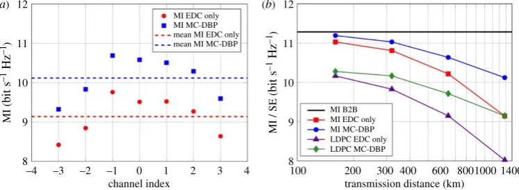
7 subchannels.Figure 9aillustrates the MI for all 7 subchannels of the DP-64QAM signal after
transmission over 1280 km of SSMF. When only EDC was employed in the receiver DSP, a
maximum MI of approximately 9.8 bit s−1Hz−1was achieved per subchannel. The MI varied by
approximately 0.2 bit s−1Hz−1over the central 3 subchannels, but reduced significantly towards
the edge subchannels. This deterioration in performance is attributed to the frequency-dependent effective number of bits in the receiver ADCs and is inherent to wide bandwidth receivers that simultaneously capture and process more than one optical channel. In order to achieve error free transmission, the code rate of the FEC implementation needs to be tailored for each subchannel, depending on the SNR after coherent detection. This will ensure that the number of information bits transmitted over the channel is maximized. MC-DBP increased the MI of each subchannel by 1 bit s−1Hz−1and, thus, yielded a mean MI for the DP-64QAM superchannel of 10.1 bit s−1Hz−1.
The corresponding average MI for all 7 subchannels, as a function of transmission distance, is
displayed infigure 9b. The B2B mean MI of the DP-64QAM superchannel was 11.3 bit s−1Hz−1
and provided the maximum achievable information rate of the system. After transmission over
160 km of SSMF and with EDC only (circles), the MI reduced to 11 bit s−1Hz−1, which decreased
further to 9.15 bit s−1Hz−1at the maximum transmission distance of 1280 km. When MC-DBP
was also used in the receiver DSP (squares), the MI increased for all recorded transmission distances. A marginal improvement in MI was achieved at a transmission distance of 160 km;
however, at the maximum reach, there was a 1 bit s−1Hz−1increase in the MI relative to the EDC
17
rsta.r
oy
alsociet
ypublishing
.or
g
Ph
il.T
ran
s.R
.So
c.A
37
4
:2
[image:18.493.79.414.108.303.2] [image:18.493.60.434.370.507.2]0140440
...
10–2
BER
outer HD-FEC threshold outer HD-FEC threshold
EDC only (pre-FEC) 1280 km EDC only (post-FEC) 1280 km
MC-DBP only (pre-FEC) 1280 km MC-DBP only (post-FEC) 1280 km
10–1
10–2
BER
10–3
–18 –16 –14 –12 –10 –8 optical launch power (dBm) outer HD-FEC threshold
EDC only (pre-FEC) 640 km EDC only (post-FEC) 640 km
–6 –4 –2 0 2
10–1
10–3
–18 –16 –14 –12 –10 –8 optical launch power (dBm)
–6 –4 –2 0 2 –18 –16 –14 –12 –10 –8
optical launch power (dBm)
–6 –4 –2 0 2
(b)
(a)
(c)
Figure 8.Pre- and post-FEC BER as functions of launch power for the central subchannel. (a) EDC only after 640 km of SSMF (RSD=5/6), (b) EDC only after 1280 km of SSMF (RSD=3/4) and (c) MC-DBP after 1280 km of SSMF (RSD=5/6).
12
(a) (b)
8
–4 –3 –2 –1 0
channel index transmission distance (km)
1 2 3 4 100 200 300 400 600 8001000 1400 9
10 11
12
MI EDC only
MI B2B MI EDC only MI MC-DBP LDPC EDC only LDPC MC-DBP MI MC-DBP
mean MI EDC only mean MI MC-DBP
8 9 10 11
MI (
bit s
–1 Hz –1)
MI / SE (
bit s
–1
Hz
–1)
Figure 9.(a) MI for each subchannel with and without MC-DBP after transmission over 1280 km of SSMF. (b) Mean MI and SE of the 7-subchannel DP-64QAM signal.
code rate of the SD-FEC implementation for each subchannel in order to achieve a post-FEC BER
below 4.7×10⁻³, which corresponds to the threshold of the outer SCC. This was performed
for each transmission distance and is also displayed in figure 9b. A constant 1 bit s−1Hz−1
penalty in the SE was incurred using the SD-FEC decoder at all transmission distances. For EDC only (triangles), the achieved SE followed the same trend as the estimated MI, reducing from 10.16 bit s−1Hz−1at a transmission distance of 160 km to 8 bit s−1Hz−1at 1280 km. Again,
MC-DBP (diamonds) provided a gain in SE of 1 bit s−1Hz−1 at the maximum reach. However,
for a fixed mean SE of 9.15 bit s−1Hz−1, EDC only achieved a transmission distance of 640 km,
18
rsta.r
oy
alsociet
ypublishing
.or
g
Ph
il.T
ran
s.R
.So
c.A
37
4
:2
0140440
...
represents a 100% reach enhancement due to MC-DBP and is in excellent agreement with the
central subchannel performance shown infigure 3.
6. Just how much can capacity be increased?
Clearly, a number of techniques can be effective in overcoming what has previously been assumed to be the Kerr nonlinearity limit, although the greatest effectiveness of the aforementioned techniques appears to be in increasing the transmission distance, where the capacity and SE can be maintained over as much as double the distances compared with a linearly compensated system. What about overall increases in the maximum fibre capacity?
Increasing the overall capacity is a major scientific challenge. Although for an unrepeated link, one which does not contain amplifiers, the capacity can be defined by the quantum limit of detection (i.e. shot noise [55]), recent publications [56,57] asserted that for any amplified link,
an upper bound on the capacity,Cmem in (3.2), is given by the log
2(1+SNR) expression for an
equivalent AWGN channel where the SNR is calculated using only the ASE noise. This result
means that the capacity of the optical fibre channel is not above a log2(1+SNR) expression, and
that dispersion and nonlinearity do not increase capacity. The implication of this result is that the best we can hope for is to ideally compensate Kerr nonlinearities and dispersion, resulting in a linear AWGN channel and under this assumption the nature of logarithmic function means that increasing power in the fibre will lead to progressively smaller increases in channel capacity.
As already mentioned, the channel capacity of a communication channel is the maximum rate at which information can be transmitted with an arbitrarily low error probability. Indeed, the recent vociferous scientific debates about the channel capacity of different channels have led to the realization that all the optical channels discussed are indeed different: they depend on fibre and amplifier type, span length and the in-span compensation scheme—such as optical phase conjugation or optical regeneration. In the case of the nonlinear channel, the channel properties are power dependent at the onset of significant nonlinearity or in the high power regime. Each of these different channels will have its own channel capacity and comparisons must be made with utmost care.
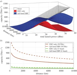
Assuming an AWGN channel one could use the GN-model to estimate the required optical power to ensure approximately a factor of 10 increase in capacity compared to the current record. Using the approximate expressions from §3, it is possible to explore the limits of what is possible through nonlinearity compensation. Using somewhat unrealistic, grossly simplifying, assumptions (e.g. wavelength-independent dispersion and loss coefficients), it is possible to explore what capacity gains might be achievable through (i) complete nonlinearity compensation and (ii) an increase in usable fibre bandwidth beyond the current EDFA bandwidth limit of approximately 35 nm (4.3 THz) to 50 THz (i.e. the full standard single-mode fibre bandwidth), approximately an order of magnitude increase. The parameters which have been assumed for
the calculations include: 2 polarizations, 50 THz bandwidth (50 Gbaud·1000 channels), C-band
(4.3 THz, 50 Gbaud·86 channels), lumped amplification with Fn=3 dB noise figure, group
velocity dispersion β2= −21.7 ps2km−1, zero PMD, nonlinear coefficient γ=1.2 W−1km−1,
attenuationα=0.2 dB km−1and 80 km per span.
The obtained results are illustrated infigure 10, where capacity is plotted against power for
two different bandwidths and distances (2000 km—a long-haul terrestrial link; and 10 000 km—
equivalent to a subsea, transoceanic system). It can be seen from figure 10 that, for an SE
of approximately 10 bit s−1Hz−1 per polarization, it would be possible to transmit 1 Pbit s−1
in the linear regime with quantum noise-limited amplifiers at the launch power of 45 dBm (approximately 30 W total launch power). This would exceed the current record for maximum
system capacity of 100 Tbit s−1by approximately a factor of 10. Taking nonlinearity of the channel
into account leads to a reduction in capacity of approximately 500 Tbit s−1. Much of this capacity
![Figure 1. (world. It should be noted that figures for SE are difficult to compare as experiments are performed over different bandwidthsbut the trend is interesting nonetheless [a) Capacity and (b) SE growth demonstrated in state-of-the art laboratory and research experiments around the3,4,9–20].](https://thumb-us.123doks.com/thumbv2/123dok_us/9465544.453018/4.493.66.431.43.189/difficult-experiments-bandwidthsbut-interesting-nonetheless-demonstrated-laboratory-experiments.webp)