ISSN: 1816-949X
© Medwell Journals, 2020
Study and Simulation of PV System Connected to Egyptian Electric Grid
1, 3
Ahmed Emad-Eldeen,
2Adel A. Elbaset,
4Mustafa Abu-Zaher and
3Ramadan Mahmoud Mostafa
1
Renewable Energy Science and Engineering Department,
Faculty of Postgraduate Studies for Advanced Science, Beni-Suef University, Egypt
2
Department of Electrical Engineering, Minia University, Elminia, Egypt
3
Electronics Department, Faculty of Industrial Education, Beni-Suef University, Beni-Suef, Egypt
4Electrical Department, Faculty of Industrial Education, Sohag University, Egypt
Abstract: This study presents a suitable method to convert the direct current to an alternating current using the
photovoltaic system to establish a connection to the grid by using three-phase designed inverter at the present time, the inverter is admitted to be the foundation stone for the semiconductors and the smart electronics technology industry, therefore, this study exposed the thermotical and simulation results for the selected controlling method for active and reactive power utilizing a high-efficiency designed three phase inverter and connect the whole system to the grid the simulation results and graphs has been carried out using dspace microLabBoxc1202 and the software program (MATLAB/Simulink), the basic motivation in this study is constructing a high performance system capable of controlling the active and reactive power in flexible method and also producing clean and renewable energy without any harmful effects on the nature or the human being also it can independently implement the injection of the active and reactive power into grid without exciting for any distortion in the wave forms. The presented control strategy for the active and reactive power is executed by using indirect power control. Where the function of the Proportional-Integral (PI) controller includes the control of error signals which represent the difference between the measured current and the source current, in order to reduce the error signal up to zero. The basic target of this study is establishing a complete system has the flexibility to control the active and the reactive and proved this effective work with accurate simulation using MATLAB to produce pure energy without distortion signals.
Key words: Three phase inverter, Space Vector Pulse Width Modulation SVPWM, active power, filter,
reactive power, photovoltaic
INTRODUCTION
Renewable energy comes into the foreground in scientific researches for discovering continuous and clean energy sources to meet the increasing demands of human being to serve all the daily need for electricity, (Kanchev et al., 2011; Suyata and Po-Ngam, 2015; Ozbay et al., 2017; Suyata et al., 2014; Sarkar and Dalvi, 2017) solar energy solved lots of energy problems. In the last decades, due to the rapid developing of the semi Industrial technology and the appearance of smart electronic devices like smart grids, three-phase inverter and also software programming all this factors provided the photovoltaic system with high performance and high quality in order to produce clean energy instead of permanent reliance on fossil fuels (Susheela and Kumar, 2017; Blaabjerg et al., 2011; Magdy et al., 2019),
conversion and transferring the energy to the grid can be applied using inverters to convert the energy form the DC form to AC form and transfer it to the grid through the DC-link, the power factor of the produced energy, the grid synchronization and the method of selected modulation are important considerations for the whole system to achieve the perfect performance for implementation of the proposed system, the three-phase designed inverter could be controlled by three synchronized frames (d-q), (α-β) and (a-b-c) (Blaabjerg et al., 2004), the park transformation is the responsible for transform currents and voltages of the three phase designed inverter into the reference frame (d-q) which is synchronized according to the voltage of the grid and that the reason for the conversion of the variables of the three phase to the DC forms, the selected method of modulation is the (SVPWM) Space Vector Pulse Width Modulation which
Corresponding Author: Ahmed Emad-Eldeen, Department of Renewable Energy Science and Engineering,
J. Eng. Applied Sci., 15 (1): 171-179, 2020
considers the most famous used technique for modulation in most of researches for the renewable energy sources (Carrasco et al., 2006; Ramonas and Adomavicius, 2013; Meneses et al., 2012; Singh et al., 2011), the main operation idea for the (SVPWM) is to control the vector of the generated voltage for the inverter and supplies the ideal switching in order to minimize the frequency and losses of switching (Yan et al., 2011; Adzic et al., 2009; Chung, 2000), the most practical features of the (SVPWM) technique are the fixed frequency and low level of harmonics, the inverter has the capability of Improving the quality of the transferred energy into grid. The dspace micro lab-box has an essential role in the simulation obtained results procedure, it’s main function is to compute the required calculation and also improving the transferring of data and observing the performance of the power controllers (Guo and Wu, 2013; Moukhtar et al., 2018; Pastor and Dudrik, 2013) and provide the results with actual simulation using MATLAB, the variable factors and the generated values for current and voltages are being detected and the actual values and instant are simulated using MATLAB/Simulink Programme and a comparison are being made between the measured values and source value to detect the error ratio and to avoid losses and distortion in the final results to achieve the optimum efficiency for the whole research, the simulation results has been performed with high accuracy.
In this study, the modulation technique of SVPWM is presented. When harmonics are founded, the (q, d) axisofgrid currents would impact performance of the grid current, so in order to overcome this problem, the (d, q) axis of currents which comprised decoupled fundamentals factors of the current controller for the grid should be changed with (d, q) axis of currents source of the grid (Yao et al., 2015).
MATERIALS AND METHODS
Connection model of a three-phase inverter to the
grid: Designing of electrical circuit for the model of
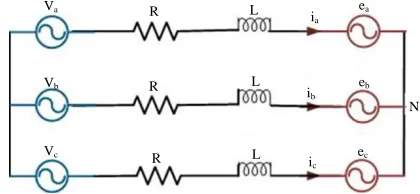
connecting three-phase designed inverter of grid is illustrated in Fig. 1. The three basic voltages of the three-phase inverter are Va, Vb, Vc, in the same time the basic voltages of the grid represented as follow: ea, eb, and ec the output currents of the inverter are: ia-ic they are being transmitted into grid.
[image:2.612.321.531.100.197.2]The using of park implementation of reverse park transformation is necessary to apply the two phases in conversion and synchronization related to the stationary frame as explained in details in following Eq. 1:
Fig. 1: Connection of three-phase inverter to the grid
(1)
a a a a
b b b b
c c c c
e i i
d
e = -R i -L i
dt
e i i
As proposed in Eq. 1, the transformation of the d-q rotating reference is performed using parks method the next functions can be obtained:
(2)
a
b
c
1 1 e
1 -
-e 2 2 2
= e
e 3 3 3
0 - e
2 2
(3)
a
a a
b
b b
c
c c
di
-L -Ri
1 1 dt
1 -
-e 2 2 2 di
= = -L -Ri
e 3 3 3 dt
0
-di
2 2 -L -Ri
dt
(4)
di
-L -Ri
e dt
=
e di
-L -Ri
dt
(5)
d -1 d
q q
X X X X
= T , = T
X X X X
Where:
X : Refers to variable
(T) : Refers to the matrix transformation
(6)
-1
cos t sin t cos t-sin t
T = ,T =
-sin t cos t sin t cos t
(7)
d
q
di
-L -Ri
e dt
= T
e di
-L -Ri
dt
Va R L i
a
ea
Vb
Vc
R
R
L
L ib
ic
eb
ec
(8)
d
q
di L
e dt Ri
= T -T -T
e di Ri
L dt
(9)
d d -1 d d
q q q q
e d i i
= -LT T -R
e dt i i
By execution differentiation we can obtain:
(10)
d d d
-1 -1 -1
q q q
i i i
d d d
T T = TT +T T
i i i
dt dt dt
(11)
-1 1 0 d -1 - sin t - cos t
TT = , T =
0 1 dt cos t - sin t
(12)
-1 0
-d
T T =
0 dt
(13)
d d d q d
q q q d q
e d i i i
= -L + L -R
e dt i -i i
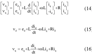
Equation 13 could be calculated in the form of state space as shown in Eq. 16. As a result, it could be easy to evaluate the inverter output voltage in the d-q frame as follow:
(14)
d d d q d
q q q d q
e d i i i
= +L - L +R
e dt i -i i
(15)
d
d d q d
di
= e +L - Li +Ri
dt
(16)
q
q q d q
di
= e +L + Li +Ri
dt
Functions 15 and 16 stand for the output voltage of the inverter in the synchronous d-q reference frame as seen in Fig. 2 and 3.
The PI controller technique for both active and reactive power depending on high quality performance in reacting with the Vd and Vq.
Proposed current controller prevalent: The most
[image:3.612.318.531.96.262.2]prevalent controller is PWM because its a multi-featured controller as it has dynamic reaction, optimum controlling strategy, accurate implementation and capable of providing sequence quantities of (ac) power, the presidential task of the current controller (PWM) voltage
[image:3.612.118.295.456.562.2]Fig. 2: Inverter output voltage in d-axis
Fig. 3: Inverter output voltage in q-axis
source inverters is to proposing a fundamental trajectory for current vector which used for the three phase load, the chosen technique for current controller has a great impact on the system efficiency and the conversion accuracy, implementation is one of the important stages for current controller to compare the measured values of the output currents of inverter with the source values to produce the output voltage of inverter with the source values to produce the output voltage of inverter, the current controller handle with the errors as input (Salem and Atia, 2014). The PI controller control the fixed quantities of dc which result from the (d-q) transformation. The PI has the ability to detect the error ratio by making comparison between both of measured and source values and then the PI works on minimizing the failure value until it reach to zero there is two constant gains related to the algorithmic estimations; (kp) the proportional gained and the (Ki) the integral gain:
(17)
d
d d q d
di
-e + Li = L +Ri = ud
dt
So, the function of d-axis current circuit could be gained using s-domain as shown in the following functions:
(18)
(s)
( s )
d
d
I 1
=
U R+LS
By mention Eq. 16:
(19)
q
q q q q
di
v -e - Li = L +Ri = uq
dt
Iq R
L LId
+ -
+ eq - +
-Vq
+
Id R
L LIq
-
ed +
- Vd
-
J. Eng. Applied Sci., 15 (1): 171-179, 2020
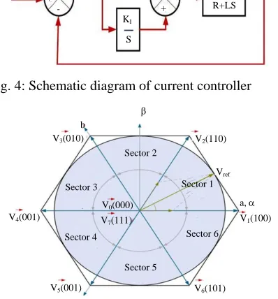
Fig. 4: Schematic diagram of current controller
Fig. 5: Swapped sectors for SVPWM
There for the function of q-axis current loop in s-domain can be realized as following:
(20)
(s)
( s )
q
q
I 1
=
U R+LS
From the functions 18 and 20 it could be predicted that the classification of the system is first order model. As illustrated in Fig. 4 the scheme diagram of current control has the ability to determine the value of source current and therefore, it could control both of active and reactive power (Lal and Singh, 2015). The fault signal react as an input for the PI, it could be calculated by making a comparing between the measured and the source values of the inverter current in the (d-q) reference frame, so, the transformation equation will be resulted from both Eq. 18 and 20 to give the following format (1/(R+LS)).
SVPWM vectors locating: The (α-β) frame voltages and
the voltages of (d-c) are used in SVPWM, the generated voltage of inverter vector as seen in Fig. 5, the source voltage is the end product of α and β items and that provide designating the sector of voltage vector and also locating its related angle as shown in Fig. 5 the vectors retard for each 60°, so, the followed technique to assign a specific sectors for the vector of reference is by
measuring vector’s angle, the inverter voltages rely on twain of active Vectors, the (V1-V6) and twain of zero Vectors (V0, V7).
System simulation prototype: The controlling strategy
which has been founded using interface programme (MATLAB\Simulink) to operate the proposed chosen technique for connecting three-phase inverter to the grid and setup the whole system including the photovoltaic array preparations as illustrated.
RESULTS AND DISCUSSION
The grid voltage and vector angel simulation are presented clearly Fig. 7, (PLL) has the reliability of creating an angle in synchronism with the grid voltage but it requires almost half cycle in order to obtain the value of required state for reaching the accurate angle. Figure 8-13: the emulation results of the six sectors of the grid vector for (SVPWM) switching pattern (Fig. 6).
Current controller simulation results: The three-phase
inverter is known to be classified as first order and that could be easily concluded from Eq. 18 and 20 and that provide the PI controller has a complete ability to control the generated inverter current in high efficiency method, the (kp) and (Ki) are the PI controller related gains where (kp) define as the proportional gain and (Ki) define as the integral gain the most appropriate method to choose the PI factors is the trial and error procedure (Ki = 300 and kp = 50) as seen in Fig. 14, 15 the resulted response of current controller for the changing step, the step change scale starts from 3A and end at 6A and occur in the case of current source for the d-axis, in the same time the current of the reference in the q-axis is set to equal zero as shown in Fig. 14, on the other hand, the q-axis step change in the case of reference current, the scale ranges from (-5A to -2A) and the d-axis is prepared to reach zero value as shown in Fig. 15, the PI is distinguishing controller as it has special qualities like: rapid, stabilized response as shown in Fig. 16 it can be clear to realize that the simulation currents for three-phase inverter have been carried out in concur with the (a-b-c) frame for the current reference for d-axis.
Active and reactive power simulation results: The
photovoltaic system produces two type of power active power and reactive power, both types are being simulated through two durations the first period is the steady state and the second is the transient period, the power factor unit operating is explained in Fig. 17, it could be realized that the active power is transferred into grid and the reactive power is set to equal zero also the voltage and the current related to phase (A) are on consensus in phase on the contrary Fig. 9-18 describes the power factor
i*dq Error
KP
Udq
+
+ +
-1 R+LS KI
S
idq
V3(010) V2(110)
b
V5(001)
V1(100)
a,
V6(101)
V4(001)
c
Sector 5 Sector 4
Sector 3
Sector 2
Sector 1
Sector 6 V0(000)
V7(111)
Fig. 6: Proposed prototype system simulation
Fig. 7: Emulation results for the voltage and angle of the grid
Fig. 8: Emulation results of the switching pattern of PWM for space vector at first sector (a) Sector, (b) Sa (c) Sb and (d) Sc
[image:5.612.86.275.276.385.2]operation when the active power prepared to equal zero and the reactive power is transferred into grid the phase A current lag behind the phase A voltage about 90° as seen in Fig. 19 in the procedure of 0.7 lag for the power factor it is clear that the phase A current lag behind the phase (A) voltage about 45° and the reactive and active power are set to be equal, it could be clearly observed that
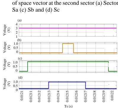
Fig. 9: Emulation results of switching pattern for PWM of space vector at the second sector (a) Sector, (b) Sa (c) Sb and (d) Sc
Fig. 10: Space vector emulation results during the third sector for PWM switching (a) Sector, (b) Sa (c) Sb and (d) Sc
the PI controller has the ability to achieve an accurate injection process for both active and reactive power to the grid (Fig. 11-18).
0.00 0.02 0.04 0.06 0.08 0.10 Time (sec)
200
100
0.00
-100
V
olt
a
va vb 2 vc
2 1 0
Volta
ge
(V)
1.0 0.5 0
1.0 0.5 0
Volta
ge
(V)
1.0 0.5 0
Volta
ge
(V)
5.80 5.81 5.82 5.83 5.84 5.85 5.86 5.87 5.88 5.89 5.90 Ts (s) ×10-3
(a)
(b)
(d)
Volta
ge
(V)
(c)
6 4 2
Volta
ge
(V)
Volta
ge
(V)
1.0 0.5 0
Volta
ge
(V)
(b)
(c)
(d)
8.80 8.81 8.82 8.83 8.84 8.85 8.86 8.87 8.88 8.89 8.90 Ts (s)
1.0 0.5 0 (a)
Volta
ge
(V)
1.0
0.5 0
Volta
ge
(V)
Volta
ge
(V)
1.0 0.5 0 (a)
(b)
(c)
Volta
ge
(V)
(d)
Volta
ge
(V)
0.0121 0.01211 0.01212 0.01213 0.01214 0.01215 0.01216 0.01217 0.01218 0.01219 0.0122
Ts (s) 1.0
0.5 0
1.0 0.5 0 4 3 2 1
Discrete 1e-06 s. Powerful Radiance
(w/m )2 2
25
Temperature (°C)
[vabc] [vabc]
Theta
[labc]
from 22 Transformation
[Vd]
[Vq]
[id] [theta]
lq
ld
l/q
Vd iq
id
Q P
[Id]
Vd
[image:5.612.90.283.437.589.2] [image:5.612.324.523.452.634.2][id]
[l-ref]
Vq
Iqref
[Vd]
[Vq] [Vd]
[Vq]
[V-means]
From15 Current control
Mean
Mean
Mean 1
CM 1
Golo 3 [v-mean]
oc
Go
OE LA
LA 1
LC
V
V
V
CA
CC CS
[vabc] [labc]
A
B
C
Garid
a2
b2
a2
[id]
J. Eng. Applied Sci., 15 (1): 171-179, 2020
[image:6.612.333.523.250.369.2]Fig. 11: Emulation results for switching patterns of PWM for space vector at the fourth sector (a) Sector, (b) Sa, (c) Sb and (d) Sc
Fig. 12: Emulation results for the switching pattern of PWM for space vector at the fifth sector (a) Sector, (b) Sa, (c) Sb and (d) Sc
Fig. 13: Emulation results of switching pattern for PWM of space vector rat the sixth sector (a) Sector, (b) Sa, (c) Sb and (d) Sc
[image:6.612.93.289.311.485.2]Fig. 14: Step change simulation results at (Id) reference and Iq estimate (d-q)
[image:6.612.337.518.408.501.2]Fig. 15: Step change simulation results at (Id) reference and Iq estimate (d-q)
Fig. 16: Step change simulation results for three phase inverters (Prodanovic and Green, 2003)
Fig. 17: (a-c) Simulation results for the process of power factor unit [Scale I:5A/div]
6 4 2 1.0 0.5 0 Volta ge ( V ) Volta ge ( V ) Volta ge ( V ) Volta ge ( V )
0.01570 0.01571 0.01572 0.01573 0.01574 0.01575 0.01576 0.01577 0.01578 0.01579 0.0158
Ts (sec) (a) (b) (c) (d) 1.0 0.5 0 1.0 0.5 0 6 5 4 3 1.0 0.5 0 Volta ge ( V ) Volta ge ( V ) Volta ge ( V ) Volta ge ( V )
0.01850 0.01851 0.01852 0.01853 0.01854 0.01855 0.01856 0.01857 0.01858 0.01859 0.01860
Ts (sec) (a) (b) (c) (d) 1.0 0.5 0 1.0 0.5 0 6 4 2 1.0 0.5 0 Volta ge ( V ) Volta ge ( V ) Volta ge ( V ) Volta ge ( V )
0.02270 0.02271 0.02272 0.02273 0.02274 0.02275 0.02276 0.02277 0.02278 0.02279 0.02280
Ts (sec) (a) (b) (c) (d) 1.0 0.5 0 1.0 0.5 0 Cu rr en t (A ) 8 6 4 2 \ 0
0.0 0.01 0
Time (sec 0.02 0.03 0.04 0.05 0
Id I
c)
.06 0.07 0.08 0.09 0 Id-ref Iq-ref I
0.1 Iq Time (sec) Cu rr en t (A ) 1 0 -1 -2 -3 -4 -5
0.0 0.01 0.02 0.03 0.04 0.05 0.06 0.07 0.08 0.09 0.1 Id Id-ref Iq Iq-ref
Time (sec) Cu rr en t (A ) 5 0 -5
0.0 0.02 0.04 0.06 0.08 0.1 Ia Ib Ic I-ref
1000 500 0 Reactive p o w er (v ar) Ac ti ve po wer (W )
0.0 0.02 0.04 0.06 0.08 0.1 0.12 0.14 0.16 0.18 0.2 Time (sec)
Voltage (V)- curre
nt (A ) (a) (b) (c) 100 0 -100 100 0 -100
[image:6.612.90.285.507.688.2] [image:6.612.331.524.538.702.2]Fig. 18: (a-c) Simulation results for the process of power factor unit at zero value [Scale I:5A/div]
Fig. 19: (a-c) Procedure of (0.7 lag) for the power factor [Scale I:5A/div]
Active and reactive power stages during (step change):
As illustrated in Fig. 20 and 21 during the operation of step change for the active power, the reactive power keeps constant at zero value, in contrast the active power keeps constant at zero value while the reactive power is undergo
change step operation as seen in Fig. 22 the active power still constant and the difference before and after the step change is that for the step change power factor value but after the step change operation occurred it can be found that the active and the reactive power have the same
100
0
-100
Reactive power
(var
)
Ac
ti
ve po
wer
(W
)
1000
500
0
0.0 0.02 0.04 0.06 0.08 0.1 0.12 0.14 0.16 0.18 0.2
Time (sec)
Voltage (V
1
)-curre
nt
(A
) 100
0
-100 (a)
(b)
(c)
la va
1000
500
0
Reactive power
(var
)
Ac
ti
ve po
wer
(W
)
1000
500
0
0.0 0.02 0.04 0.06 0.08 0.1 0.12 0.14 0.16 0.18 0.2
Time (sec)
Voltage (V
1
)-curre
nt
(A
) 100
0 -100
(a)
(b)
(c)
[image:7.612.115.502.96.357.2] [image:7.612.112.500.399.630.2]J. Eng. Applied Sci., 15 (1): 171-179, 2020
Fig. 20: (a-c) Active power simulation results during step change, [Scale I:5A/div]
Fig. 21: (a-c) The simulation results for step change in the reactive power whereas the active power is adjusted to be zero [Scale I:5A/div]
[image:8.612.319.524.93.228.2]Fig. 22: (a-c) The simulation results of the changing step for the reactive power while the active power remains fixed [Scale I:5A/div]
Fig. 23: Simulation results of changing step for the active and reactive power from the power factor unity to the 0.7 lag PF process, [Scale I:3A/div] value, so, the in injected current is lags behind about 45° from the 0.7 lag voltage Fig. 23 explains that it could be easily to achieve the steady state without the utilization of over shooting and the required time to perform that is about one millisecond, all this results leads to that the proposed technique has the complete reliability to control both of active and reactive power in steady and high accurate performance.
CONCLUSION
This research proposed a complete system for a photovoltaic structure connected to a three-phase inverter, this system has a lots of advantages like high quality, accuracy and also the generated power is clean and renewable the selected model for the three phase inverter has been designed and provided with the appropriate software programming the basic electrical circuit has been built to operate the optimal controlling system the selected control is PI it has many advantages such as quick dynamic response, the ability of controlling the active and reactive power in order to reach the desired results.
REFERENCES
Adzic, E., Z. Ivanovic, M. Adzic and V. Katic, 2009. Maximum power search in wind turbine based on fuzzy logic control. Acta Polytech. Hungarica, 6: 131-149.
Blaabjerg, F., M. Liserre and K. Ma, 2011. Power electronics converters for wind turbine systems. IEEE. Trans. Ind. Appl., 48: 708-719.
Blaabjerg, F., Z. Chen and S.B. Kjaer, 2004. Power electronics as efficient interface in dispersed power generation systems. IEEE Trans. Power Electron., 19: 1184-1194.
Carrasco, J.M., L.G. Franquelo, J.T. Bialasiewicz, E. Galvan and R.P. Guisado et al., 2006. Power-electronic systems for the grid integration of renewable energy sources: A survey. IEEE Trans. Ind. Electron., 53: 1002-1016.
Reactive
p
o
w
er
(v
ar)
Ac
ti
ve
po
wer (W
)
0.0 0.02 0.04 0.06 0.08 0.1 0.12 0.14 0.16 0.18 0.2 Time (sec)
Voltage (V)- curre
nt
(A
)
la va 1000
500
0
200 100 0 -100
100 0 -100
(a)
(b)
(c)
100
0
-100
1000
500
0
100 0 -100
(a)
(b)
(c)
Reactive
p
o
w
er
(v
ar)
Ac
ti
ve
po
wer (W
)
0.0 0.02 0.04 0.06 0.08 0.1 0.12 0.14 0.16 0.18 0.2 Time (sec)
Voltage (V)- curre
nt
(A
)
la va
1000
500 0
1000 500 0
100 0 -100
Reactive
p
o
w
er
(v
ar)
Ac
ti
ve
po
wer (W
)
Voltage (V) curre
nt
(a
)
(a)
(b)
(c)
0.0 0.02 0.04 0.06 0.08 0.1 0.12 0.14 0.16 0.18 0.2 Time (sec)
la va
150
100 50
0
-50 -100
-150
0 0.02 0.04 0.06 0.08 0.1 0.12 0.14 0.16 0.18 0.2 Time (sec)
Curre
nt (A),
Vo
lt
ag
e (V
)
[image:8.612.85.268.97.269.2] [image:8.612.96.270.313.485.2] [image:8.612.88.279.537.688.2]Chung, S.K., 2000. A phase tracking system for three phase utility interface inverters. IEEE Trans. Power Electron., 15: 431-438.
Guo, X.Q. and W.Y. Wu, 2013. Simple synchronisation technique for three-phase grid-connected distributed generation systems. IET. Renewable Power Gener., 7: 55-62.
Kanchev, H., D. Lu, F. Colas, V. Lazarov and B. Francois, 2011. Energy management and operational planning of a microgrid with a PV-based active generator for smart grid applications. IEEE. Trans. Ind. Electron., 58: 4583-4592.
Lal, V.N. and S.N. Singh, 2015. Control and performance analysis of a single-stage utility-scale grid-connected PV system. IEEE. Syst. J., 11: 1601-1611.
Magdy, G., G. Shabib, A.A. Elbaset and Y. Mitani, 2019. Renewable power systems dynamic security using a new coordination of frequency control strategy based on virtual synchronous generator and digital frequency protection. Intl. J. Electr. Power Energy Syst., 109: 351-368.
Meneses, D., F. Blaabjerg, O. Garcia and J.A. Cobos, 2012. Review and comparison of step-up transformerless topologies for photovoltaic AC-module application. IEEE. Trans. Power Electron., 28: 2649-2663.
Moukhtar, I., A.A. Elbaset, A.Z. El Dein, Y. Qudaih and Y. Mitani, 2018. Concentrated solar power plants impact on PV penetration level and grid flexibility under Egyptian climate. AIP. Conf. Proc., Vol. 1968, 10.1063/1.5039224
Ozbay, H., S. Oncu and M. Kesler, 2017. SMC-DPC based active and reactive power control of grid-tied three phase inverter for PV systems. Intl. J. Hydrogen Energy, 42: 17713-17722.
Pastor, M. and J. Dudrik, 2013. Predictive current control of grid-tied cascade H-bridge inverter. Automatika, 54: 308-315.
Prodanovic, M. and T.C. Green, 2003. Control and filter design of three-phase inverters for high power quality grid connection. IEEE. Trans. Power Electron., 18: 373-380.
Ramonas, C. and V. Adomavicius, 2013. Research of the converter control possibilities in the grid-tied renewable energy power plant. Elektronika ir Elektrotechnika, 19: 37-40.
Salem, M. and Y. Atia, 2014. Design and implementation of predictive current controller for photovoltaic grid-tie inverter. WSEAS. Trans. Syst. Contr., 9: 597-605.
Sarkar, D.U. and H.S. Dalvi, 2017. Modeling and designing of solar photovoltaic system with 3 phase grid connected inverter. Proceedings of the 2017 2nd International Conference for Convergence in Technology (I2CT’17), April 7-9, 2017, IEEE, Mumbai, India, pp: 1018-1023.
Singh, M., V. Khadkikar and A. Chandra, 2011. Grid synchronisation with harmonics and reactive power compensation capability of a permanent magnet synchronous generator-based variable speed wind energy conversion system. IET. Power Electron., 4: 122-130.
Susheela, N. and P.S. Kumar, 2017. Performance evaluation of carrier based PWM techniques for hybrid multilevel inverters with reduced number of components. Energy Procedia, 117: 635-642. Suyata, T.I. and S. Po-Ngam, 2014. Simplified active
power and reactive power control with MPPT for three-phase grid-connected photovoltaic inverters. Proceedings of the 2014 11th International Conference on Electrical Engineering/Electronics, Computer, Telecommunications and Information Technology (ECTI-CON’14), May 14-17, 2014, IEEE, Nakhon Ratchasima, Thailand, pp: 1-4. Suyata, T.I., S. Po-Ngam and C. Tarasantisuk, 2015. The
active power and reactive power control for three-phase grid-connected photovoltaic inverters. Proceedings of the 2015 12th International Conference on Electrical Engineering/Electronics, Computer, Telecommunications and Information Technology (ECTI-CON’15), June 24-27, 2015, IEEE, Hua Hin, Thailand, pp: 1-6.
Yan, L., X. Li, H. Hu and B. Zhang, 2011. Research on SVPWM inverter technology in wind power generation system. Proceedings of the 2011 International Conference on Electrical and Control Engineering, September 16-18, 2011, IEEE, Yichang, China, pp: 1220-1223.

![Fig. 19: (a-c) Procedure of (0.7 lag) for the power factor [Scale I:5A/div]](https://thumb-us.123doks.com/thumbv2/123dok_us/9518652.457328/7.612.115.502.96.357/fig-procedure-lag-power-factor-scale-i-div.webp)
![Fig. 23: Simulation results of changing step for the activeand reactive power from the power factor unityto the 0.7 lag PF process, [Scale I:3A/div]](https://thumb-us.123doks.com/thumbv2/123dok_us/9518652.457328/8.612.88.279.537.688/simulation-results-changing-activeand-reactive-factor-unityto-process.webp)
