Nonequilibrium BKT transition in microcavity polaritons

(1)

warwick.ac.uk/lib-publications

A Thesis Submitted for the Degree of PhD at the University of Warwick

Permanent WRAP URL:

http://wrap.warwick.ac.uk/88602

Copyright and reuse:

This thesis is made available online and is protected by original copyright.

Please scroll down to view the document itself.

Please refer to the repository record for this item for information to help you to cite it.

Our policy information is available from the repository home page.

(2)

Nonequilibrium BKT Transition in Microcavity

Polaritons.

by

Galbadrakh Dagvadorj

Thesis

Submitted to the University of Warwick for the degree of

Doctor of Philosophy

Department of Physics

(3)

Acknowledgments

(6)

Declarations

I declare that the content of this thesis is original work except where referenced within the text and has not been submitted as part of any other degree or qual-ification. Chapters 1, 2 and 3 provide a background to the field, the information for which was gathered from the texts cited throughout. Chapter 4 is based on the following paper:

• G. D. Dagvadorj, J. M. Fellows, S. Matyja´skiewicz, F. M. Marchetti, I. Caru-sotto, and M. H. Szyma´nska , Non-equilibrium phase transition in a two-dimensional driven open quantum system, Physics Review X 5, 041028, De-cember 2015

The entirety of the work was conducted under the supervision of Dr. M. H. Szyma´nska and the content of the chapters highlighted above was performed in collaboration with the indicated authors. The thesis was typeset with LA_{TEX 2}_ε_{and the}

(7)

Abstract

(8)

List of Tables

1.1 Comparison of characters of atoms, excitons and polaritons, adopted from [1]. . . 2 3.1 Comparison between GaAs exciton parameters in the reduced mass

approximation and those of the Hydrogen atom. . . 37 4.1 Characteristics for each of the GaAs quantum wells and for the

(9)

List of Figures

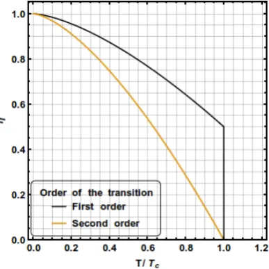
2.1 The Bose-Einstein distribution function as a function of energy for different values of the fugacity ζ. . . 6 2.2 Variation of the order parameter as a function of a control parameter

in first and second order phase transitions. Here, η is the order pa-rameter with the temperature playing the role of the control papa-rameter. 12 2.3 Cartoon for rotating liquid helium experiment. The liquid has a

or-ange colour, and is confined between two concentric cylinders, so that it does not penetrate the central cylinder, which is shown in black. The cylinders can rotate around their axis. . . 23 3.1 Schematics of an idealised bandstructure for a direct gap

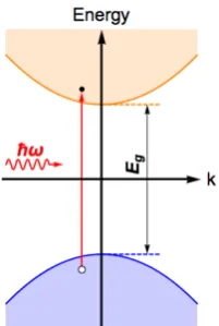
semicon-ductor which consist of a completely filled valence band (blue) and an empty conduction band (orange). The electron excitations in the direct gap semiconductors illustrated by the arrow, in the absence of electron-electron in teractions, where an electron is exciting from the valence band to the conduction band, leaving a positively charged hole in the valence band. . . 38 3.2 Cartoon of a hydrogen like discretized energy bands of excitons in a

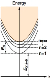
direct gap semiconductor given by equation (3.2). The most upper dashed line is the energy level ofE(∞), is the minimum energy of the continuum state -upper bound of discrete energy level and which is equal to band gapEg. . . 39

(10)

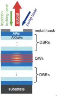
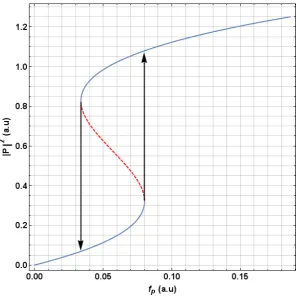
3.4 Semiconductor microcavities are nanostructures that consist of a pla-nar Fabry-Perot cavity with one or more embedded quantum struc-tures (wells, wires, dots etc), sandwiched between two Bragg mirrors. 41 3.5 The S curve: Pump-polariton population as a function of the

pump-power. The red dashed line represents the unstable region. . . 52

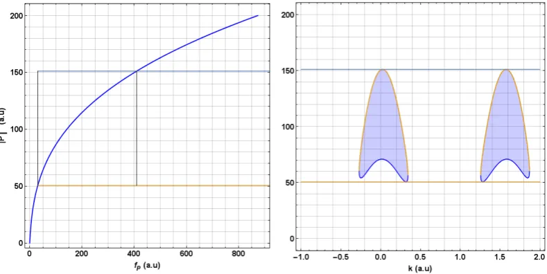
3.6 Right panel. The blue line: Population of pump mode as a function of pump-power in the optical limiter regime. The orange (light blue) line: Pump mode population at the lower (upper) OPO threshold. Black vertical lines: Upper and lower threshold pump-powers. Left panel. Population of pump mode as a function of signal momenta. In the shaded regions, pump-only states are unstable. . . 54

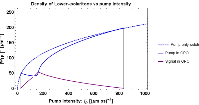
3.7 Mean field OPO phase diagram. Blue dashed-stable pump-only states. Blue solid-unstable pump-only states. Purple-Population of signale mode. Black vertical-Upper and lower threshold, same lines as in Figure 3.6. . . 55

4.1 Noise consistence. Taken 96 realizations and the step-size of the inte-gration is dt0 = 0.01. . . 64

4.2 The numerical convergence on different grids. . . 65

4.3 Mean-field steady state: convergence in time. . . 67

4.4 OPO in MF regime . . . 68

4.5 Schematic illustration of the parametric pumping scheme. . . 70

4.6 Correlation function averaged over different numbers of realisations. 72 4.7 Convergence in time of the average signal density. . . 73

4.8 Convergence in time of the average number of vortices. . . 73

4.9 Time versus stochastic realisations averaging. . . 74

4.10 Correlation function averaged over different numbers of realisations. 76 4.11 The numerical convergence on different grids. . . 77

4.12 Phase and vortices of the signal for increasing pump power . . . 78

4.13 The phase diagram. . . 80

4.14 Algebraic and exponential fits to the correlation function. . . 82

4.15 Algebraic and exponential decay of the first order correlation function across the BKT transition. . . 83

(11)

5.2 Average number of vortice across the phase transition. Left: accross lower OPO threshold. Right: accross upper OPO threshold. . . 87 5.3 First order spatial correlation function of the four components. . . . 87 5.4 Left: Full vortex - vortex in each circular polarizations. Right half

(12)

Chapter 1

Introduction

At low temperatures many physical systems undergo a phase transition from a dis-ordered to an dis-ordered state in which phase coherence is spontaneously established. This spontaneously formed coherence allows pure quantum mechanical effects to be visible at mesoscopic and even macroscopic scales. The most representative ex-amples of these effects are superconductivity and superfluidity and, more recently, Bose-Einstein condensation (BEC) [2]. Each of these phenomena have been deep-ened our fundamental understanding of many body physics, and have been led to novel research areas and experimental tools as well as applications.

BEC was originally a theoretical concept, and only gained application when its connection to the superfluidity of liquid Helium was realised [3]. Recent exper-iments in atomic gases have enabled the realisation of equilibrium BEC [4, 5], via cooling atoms then trapping only atoms with low energies, and have lead to much interest in the subject. However, atoms are heavy particles so one has to reach very low temperature to condensate. Moreover, increasing atomic gas density is quite challenging task because once density increases atoms bind together and form molecules which are more difficult to control. Nowdays, experiments on atomic gases which are probing many-body physics effects are facing a high level of sophistication [6], so the limitations of the system start showing up. This is specially true for low-dimensional systems where the fluctuations and interactions are play an impor-tant roles. In particularly, the true lower dimensional systems are not yet possible in atomic gases, only engineered lattice potentials with very periodic structures are possible in current experiments.

(13)

Systems Atoms Excitons Polaritons Effective mass: m∗ ∼103me ∼10−1me ∼10−5me

Bohr radius: aB 10−1

◦

A 102A◦ 102A◦ Particle spacing: n−1/d 103A◦ 102A◦ 1.0µm

Critical temperature: Tc 1.0nK−1.0µK 1.0mK−1.0K (1−300)K

Termalization/Lifetime: τC,T 1.0ms 10.0ps (1.0-10.0)ps

Table 1.1: Comparison of characters of atoms, excitons and polaritons, adopted from [1].

with excitons in a quantum well placed inside. As a result, both particles lose their independent characters and are better described in terms of new two-dimensional quasiparticles called exciton-polaritons. This solid state implementation promises a solution to many of the obstacles presented by its atomic counterpart, and is there-fore a very interesting system for studying many-body collective phenomena as well as possible applications in the field of quantum photonics. Due to the strong con-finement along growth direction of the semiconductor exciton-polaritons are ideally two-dimensional system, however with more advanced growth techniques it could be even one- or zero-dimensional system.

Exciton-polaritons have light mass due to the photonic component and there-fore Bose-Einstein condensation is expected at higher temperatures [1, 7]. The main relative properties of atomic, exciton and exciton-polariton gases for Bose-Einstein condensation are summarised in Table 1.1. Because of no perfect confinement of cavity, cavity photons have short lifetime, continuously leaks out of cavity, so ther-mal equilibrium cannot be reached in this system. Because of this continuous lose system one has to be also continuously fed by fresh particles at same rate so that a steady state with constant particle density is maintained. Indeed, this particularity of the system allows us to studies that would be otherwise impossible, and raises new questions, such as what superfluidity means in a non-equilibrium context.

(14)

(15)

Chapter 2

Background

The aim of this chapter is to describe superfluidity in two-dimensional bosonic equi-librium systems [2]. Although the theory developed in this chapter is not directly applicable to the system of exciton-polaritons, due to its intrinsically non-equilibrium nature, it provides a good account on what superfluidity is and reveals its important features, such as quantized vortices.

We will start with tree-dimensional non-interacting Bose gas to introduce the basic concepts of Bose-Einstein Condensation (BEC) and superfluidity, then discuss their properties under rotations and weak interactions. After showing the absence of a true long range order and a true condensate at finite temperatures, the Hohenberg-Mermin-Wagner theorem, we present the Berezinskii-Kosterlitz-Thouless theory of superfluidity in two dimensional systems.

2.1 Three dimensional Bose gas and Bose-Einstein

con-densation

(16)

liquid phases. The first application of BEC to a physical system was by F. London in 1938 when he proposed [3, 12] that theory of BEC could explain the recent discovery of superfluid phenomena that had just been observed in liquid helium [13, 14]. The first unambiguous realization of BEC itself was achieved more than half a century after first theoretical propose in weakly interacting dilute atomic gases [4, 15].

2.1.1 Non-interacting Bose gas

The properties of ideal, non-interacting Bose gases are essentially determined by the particle quantum statistics. Quantum statistics determines how particles distribute over all possible quantum states, depending on the symmetry of the wave function upon a permutation of the particles. In the grand canonical ensemble - a system that is in contact with a large reservoir, such that it can exchange energy and particles with the reservoir - one can start with the Bose-Einstein distribution function which lead us to a criterion for BEC then we define the critical temperature and the condensate fraction for the homogeneous gas. The distribution function f(ν) for

the average occupation of a single particle stateν with energyν is

f(ν) =

1

exp [(ν−µ)/(kBT)]−1

, (2.1) where kB is the Boltzmann constant. The chemical potential µ is determined as a

function ofN-total number of particles and the temperatureT by the condition that the total number of particles be equal to sum of the occupancy of individual levels. Sometimes it is more convenient to work in terms of thefugacity which is given by

ζ = exp(µ/kBT). For free bosons, this quantity is equal to unity bellow transition

temperature and less than unity above. In Figure 2.1 the distribution function (2.1) is shown as a function of energy for different fugacities.

At high temperatures the chemical potential lies well bellow the energy of the lowest single particle state0. Hence, in this limit, the average occupation number

of any state is much less than unity. When temperature decreases, the chemical potential increases together with the average occupation numbers. However, because the average occupation numberN0 of the lowest single particle state with energy0

N0 =

1

exp [(0−µ)/(kBT)]−1

(17)

Figure 2.1: The Bose-Einstein distribution function as a function of energy for dif-ferent values of the fugacityζ.

1

exp [(ν−0)/(kBT)]−1. The total number of particles Nex in the excited states is just

the sum

Nex =

X

ν6=0

Nν. (2.3)

IfNexis less than total number of particlesN, the remaining particles must be

accu-mulated in the lowest single-particle state, ground state, whose occupation number can be arbitrarily large since N0 diverges as µ→ −0, so the system exhibits

Bose-Einstein condensation. Knowledge about the quantum statistics, i.e. the distribution function of the particles, allows one to derive some average quantities like the total number of particles and average energy in the system

N =X

ν

f(ν) and E=

X

ν

νf(ν). (2.4)

In general, in order to calculate thermodynamic properties of gases, the above sums over the discrete energy levels are usually replaced by integrals, and one needs to use a density of states in which the details of the level structure are smoothed out:

N =X

ν

f(ν)≈

Z ∞

0

(18)

describes the probability of occupying a certain state, the concept of the density of states is employed for the states which are actually available in the system under consideration. Integrating the product of the two yields then the total number of particles. In order to replace the sum by an integral the density of states is required to be high. However, for a vanishing density of states this replacement might be problematic.

Density of states

Heisenbergs uncertainty relation dictates the quantisation of the phase space in quan-tum mechanics. In that respect, there is one quanquan-tum state per phase space cell oc-cupying a volume equal to (2π~)3. Ascribing to a phase space region the real volume

∆V = ∆x∆y∆z and the volume 4₂πp3 in momentum space which contains states with momenta smaller than p, one can express the total number of states having energy less than = ₂p_m2 as

G() = V

4 3πp

3

(2π~)3 =V

√

2 3π2_~3(m)

3/2_. _(2.6)

Hence, the density of statesg() for a homogeneous system in three dimensions can be written as

g() = dG()

d =V

√

2 3π2_~3m

3/21/2_. _(2.7)

The density of states in the majority of cases can be expressed as a function of the energy in the form

g() =Cαα−1, (2.8)

whereCαis a constant. For the homogeneous case in ddimensions we findα=d/2,

while for the harmonic oscillator inddimensions one has α=d. It is worth noting here that the density of states for the homogeneous two dimensional system proves to be independent of the energy. This implies that Bose condensation in a two dimensional box can only take place at zero temperature.

We will now study the behaviour of the expression (2.5) keeping the temper-ature T fixed but adding progressively more particles to the system. The density

n=N/V will consequently rise and we can write

n= N

V =A

Z ∞

0

d

1/2

exp

−µ kBT

(19)

where we have defined the prefactor A = √2m3/2/(3π2~3). An increase in the

density follows from an increase in the chemical potential. Since the latter can only be negative (otherwise f() would yield unphysical negative occupation numbers), the maximum allowed value is zero if the minimum energy0 is set to zero. A further

implication is that the density of the system appears to be bound by a maximum value:

nc=n(µ= 0) =A

Z ∞

0

d

1/2

exp_k

BT

=A(kBT)

3/2

Z ∞

0

dx x

1/2

ex₋₁, (2.10)

with the substitutionx=/(kBT). We can evaluate this integral with recourse to the

Gamma function Γ(α) and the Riemann zeta functionζ(α): R∞

0 dx xα−1

ex₋₁ = Γ(α)ζ(α).

In our case we haveα= 3/2 and we then find

nc=AΓ(3/2)ζ(3/2) = 2.3A. (2.11)

This result is manifestly unphysical, as the density of the system is bound in spite of the increase in the particle number. We might then ask what happens to the particles we add? The mistake we committed occurred when we replaced the sum by an integral, which is invalid when the density of states is small. In fact, this is the case for a three-dimensional homogeneous system. In order to correct this mistake, we ought to separate the lowest energy state from all the excited states, so that

n=n0+nex=

1

V

1

e−µ/(kBT)−1+A

Z ∞

0

d

1/2

exp

−µ kBT

. (2.12)

If we now consider the limit µ→ 0, corresponding to an increase in the number of particles available in our system, the second term will be bound to nc, which is the

critical density, while the first term,n0, can grow without bounds as _V1 _e→10₋₁ → ∞.

The ground state of the system will accommodate any additional particle in excess of the critical density. The ground state then becomes macroscopically occupied, giving rise to the phenomenon ofBose-Einstein condensation (BEC).

(20)

point in phase space which becomes macroscopically occupied.

Phase space density at the phase transition

It proves useful to write the critical densityncas a function of the thermal de Broglie

wavelengthλT =

q

2π~2

mkBT, which can be construed as the spatial extent of a particle

wave function. We can then write

nc= 2.3A(kBT)3/2 = 2.3

2

√

π

1

λT

. (2.13) The critical density at which BEC sets in is thus reached if the interparticle distance is of the order of the thermal de Broglie wavelength. At that density the correspond-ing wave packets of the individual particles begin to overlap, and the system Bose condenses under the influence of quantum statistics.

Transition temperature and condensate fraction

We will now give expressions for the critical temperatureTc, below which the ground

state of the system becomes macroscopically occupied, and for the corresponding condensed atomic fractionn0 =N0/N below the critical temperature. We simplify

our treatment by setting 0 = 0.

In order to find the critical temperature we fix the system at the critical point, where all the particles are occupying the excited energy states with density

n= N

V =

Nex

V =AΓ(3/2)ζ(3/2)(kBTc)

3/2_, _(2.14)

such that

kBTc≈3.31~ 2_n2/3

m . (2.15)

The expression for condensate fraction n0 can now be derived from

n=n0(T) +nex(T) =n0(T) +AΓ(3/2)ζ(3/2)(kBT)3/2. (2.16)

If a BEC is formed in the system, the second term will remain fixed at the critical density nc. We can replace the coefficients of the second term making use of the

expression (2.14), to find

n=n0(T) +n

T Tc

3/2

(21)

The condensate fraction, finally, reads

n0=

N0

N = 1−

T Tc

3/2

. (2.18) In the next part we will give the general description of continuous phase transitions and underline their key concepts related to BEC, in particular symmetry breaking and the concept of the order parameter.

2.1.2 Spontaneous symmetry breaking, order parameter and long range order

Phase transitions are the cooperative phenomena associated with a global change of structure and the related physical properties of a system which is subject to a continuous change of a certain external conditions, such as temperature, pressure, or others. A phenomenological theory of second order phase transitions was proposed by Landau in 1937 [16] and since then has attracted a lot of interest because of its simplicity and universality in terms of its application. The Landau theory can be used to describe a wide range of phase transitions. Notable examples include the fer-roelectric, structural and magnetic, but equally the superconducting and superfluid phase transitions. The arguments are based on thermodynamic principles through the unification of various mean field theories. In that context we give emphasis on two closely related important, general concepts: broken symmetry and the order parameter.

Broken symmetry

Symmetry breaking very often accompanies a phase transition. Here, symmetry is to be understood as the invariance of certain physical quantities under some operations, which may form a closed set (called a symmetry group). The physical properties of the liquid state, for example, are invariant to arbitrary translations and rotations, i.e. invariant under the action of the elements in the Euclidean group E(3).

A physical system is described by a Hamiltonian. The symmetry possessed by that system is reflected in the invariance of the Hamiltonian under a particular class of transformations.

(22)

symme-try. Broken symmetry refers to a situation in which a particular state does not have the full symmetry possessed by the system Hamiltonian. A well-known example is that of a magnetic system: at temperatures above the Curie temperature the system has zero magnetization for zero external field; it is therefore symmetric, i.e. there is no preferred direction of the magnetization. As the temperature is lowered below the Curie temperature, however, a spontaneous magnetization develops in a specific direction, breaking down the full anterior symmetry.

We will now discuss a structural phase transition. Here, the symmetry may be transformed from the liquid to a crystalline state the temperature decreases. This process breaks continuous translation and rotation symmetries. The symmetry group of the broken symmetric state is a subgroup of the initial group in numerous cases of second order phase transitions,

We can distinguish between two types of broken symmetries: the spontaneous breaking where the HamiltonianH remains invariant, and the externally disturbed,

H→H+H0, where H0 is a perturbation addition to the original HamiltonianH.

Order parameter

We shall now proceed to give a quantitative description of phase transitions that occur in a given system. Invoking the concept of broken symmetry we discussed above, we can classify phase transitions through the loss or gain of some symmetry elements subject to the change of macroscopic system variables. When a system is transformed from a high symmetry to a low symmetry phase, there is a physical quantity η, called the order parameter, varying in such a fashion that it assumes a zero value in the high symmetry phase and non-zero values in the low symmetry phase. In the famous example of a magnetic transition, for instance, the parameterη

may be taken as the macroscopic magnetic moment per unit volume of a ferromagnet undergoing the transition.

Since the order parameter is intimately related to the symmetry of a system, the high symmetry phase can be called thedisordered phase, and the low symmetry phase the ordered phase. In the spirit of the Landau theory of phase transitions, a macroscopic order parameter η may be defined to measure the ordered phase below the transition temperatureTc. We consider this variableηa thermodynamic variable,

namely the ensemble average of a microscopic variableσi, which is a function of the

(23)

disordered phase, those variables σi are usually performing a fast random motion

with their time average hσiit vanishing at each point independently of the site i.

Below Tc, on the other hand, the variables are correlated while performing slow

[image:23.595.212.406.257.451.2]

motion. Their spatial distribution dominates the behaviour of the ordered phase. We will emphasize once more that the symmetry of a system is altered only when η becomes different to zero. Any nonzero value of the order parameter, even arbitrarily small, brings about a lowering of the symmetry. Although the change of symmetry is always abrupt, the order parameter can vary in two distinct fashions. The order of the transition is decided upon the manner by which the symmetry is

Figure 2.2: Variation of the order parameter as a function of a control parameter in first and second order phase transitions. Here, η is the order parameter with the temperature playing the role of the control parameter.

broken. Generally speaking, there are phase transitions of two kinds. One is the

first order phase transition, in which the order parameter varies discontinuously in the region of the transition temperature Tc. The two symmetry groups for the

high symmetry phase and low symmetry phase are not necessarily subject to any group-subgroup relationship.

(24)

We have seen in the previous sections that the condensate fraction N0/N

in a BEC is different to zero below the critical temperature Tc, and tends to zero

above that temperature value. It appears then that the condensate fraction N0/N

would be an anticipated choice for the order parameter. It will prove more useful, however, to define a single quantity providing information simultaneously on the number of particles in the condensate as well as on and the single particle state in which condensation takes place. With that in mind, if ψ0(r) is the wavefunction

of the lowest energy state with populationN0, we define the order parameter for a

BEC transition occurring in a non-interacting Bose gas as below

Ψ(r)≡pN0ψ0(r). (2.19)

The BEC is a second order phase transition since the order parameter gradually increases when crossing the transition temperature, while the spontaneous breaking of symmetry reflects the gauge symmetry.

Long range order

In the most general case, the system we are considering can be described by a statistical mixture of mutually orthogonal states m with weightspm. We can then

define the one-body density matrix as

n(1)(r,r0) ≡ NX

m

pm

Z

dr2dr3...drNψ∗m(r,r2, ..,rN)ψm r0,r2, ..,rN

≡ Dψˆ†(r) ˆψ(r0)

E

. (2.20)

Since the operator n(1)(r,r0) is Hermitian, it can be diagonalized, with

n(1)(r,r0) =X

i

niχ∗i(r)χi(r0). (2.21)

The phenomenon of BEC occurs when only one of the above eigenvalues ni is of

order N, while all the rest are of the order of unity. We label the macroscopically occupied state that corresponds to the eigenvalue ni as i ≡ 0 and its occupation

number asni=0 ≡N0. We are able then to define the order parameter similarly to

(2.19)

Ψ(r)≡pN0χ0(r). (2.22)

(25)

the order of unity. On the other hand, if two or more eigenvaluesni are of orderN,

the system exhibits a so-calledfragmented BEC.

The diagonal part of the one-body density matrix (r=r0) yields the particle density, while the off-diagonal part (r 6= r0) measures the established coherence between distant points in space. In order to understand its behaviour we consider the momentum distribution

n(p) =Dψˆ†(p) ˆψ(p)E, (2.23) where ˆψ(p) = (2π~)−3/2Rdrexp[irp/~] ˆψ(r) is the expression of the field operator

in momentum (Fourier) space. In a homogeneous system, the elements n(1)(r,r0) depend only on the relative distance s≡r−r0 between the particles. The Fourier transform of the momentum distribution reads

n(1)(s) = 1

V

Z

dpn(p)e−isp/~_, _(2.24)

withV the total volume of the homogeneous system. In a non-interacting BEC, the lowest energy state with zero momentum is macroscopically occupied, so the density distribution exhibits the singular behaviour

n(p) =N0δ(p) + ˜n(p), (2.25)

where ˜n(p) is a smooth function. The long-distance behaviour of n(1)(s) is then determined predominantly by the delta function in the first term. In particular, the momentum distribution approaches a non-zero value as s→ ∞

n(1)(s)s→∞ →

N0

V . (2.26)

This behaviour is termed asoff-diagonal long-range order.

The distribution functionn(1)(s) provides information on the thermodynam-ics of the system and the mechanism by which order is established. We refer the reader to section 2.2 for more details on the case of a two-dimensional Bose gas, and the calculation of n(1)(s) in several limiting cases.

(26)

We also define for convenience the first order correlation function g(1)(s), takingn(1)(s) and normalizing by the local particle density

g(1)(r) =

D

ˆ

ψ†(r+s) ˆψ(r)

E

r D

ˆ

ψ†₍_r₊_s_{) ˆ}_ψ₍_r₊_s₎E D_ψˆ†₍_r_{) ˆ}_ψ₍_r₎E

. (2.27)

Because of their close connection the two quantities are often used interchangeably.

2.1.3 Interacting Bose gas

In order to describe the behaviour of an interacting system we cannot resort to a collection of particles each one occupying a single-particle state. One instead employs a many-body state wavefunction ψn(r1,r2, ..,rN), where N is the total number of

particles,riis the radius vector of thei-th particle, and the functionψnis symmetric

under the exchange of any index pair (here we are considering Bose statistics). We describe quantitatively such an interacting BEC state by making the simplest possible ansatz for the many-body wavefunctionψN in a system ofN bosons

all occupying the same state

ψN(r1,r2, ...,rN;t) = N

Y

i=1

χ0(ri, t). (2.28)

In the absence of interactions, the wavefunctions χ0(ri, t) would satisfy the time

dependent Schr¨odinger equation

i~∂χ0(r, t)

∂t =

− ~

2

2m∗∇

2₊_V

ext(r, t)

χ0(r, t), (2.29)

where m is the single particle mass and Vext(r, t) is a potential which is externally

applied to the system. The contact interaction generates an effective potential of the form N0g|χ0(r, t)|2. Adding this nonlinear term in (2.29) yields

i~∂χ0(r, t)

∂t =

− ~

2

2m∗∇

2₊_V

ext(r, t) +N0g|χ0(r, t)|2

χ0(r, t). (2.30)

(27)

finally at the (time-dependent) Gross-Pitaevskii equation (GPE)

i~∂Ψ(r, t)

∂t =

− ~

2

2m∗∇

2₊_V

ext(r, t) +g|Ψ(r, t)|2

Ψ(r, t). (2.31) If the external potentialVext(r, t) is time-independent, then (2.31) admits solutions

of the form Ψ(r) exp(−iµt/~), where Ψ(r) satisfies the time-independent GPE

µΨ(r) =

− ~

2

2m∗∇

2₊_V

ext(r, t) +g|Ψ(r)|2

Ψ(r). (2.32) The equation (2.32) can also be derived [17] from the requirement that Ψ(r) mini-mizes the total energy functional

E = ~

2

2m∗

Z

|∇Ψ(r)|2_dr₊

Z

Vext(r)|Ψ(r)|2dr+

1 2g

Z

|Ψ(r)|4_dr, _(2.33)

under the constraint (normalization condition)

Z

|Ψ(r)|2dr=N, (2.34) where N is the total particle number. The time dependence is fixed by the chem-ical potential, µ, which is just the Lagrange multiplier associated with the particle number conservation (2.35), namely

µ= ∂E

∂N. (2.35)

In a spatial region with a density n0(r) =|Ψ(r)|2 remaining nearly constant,

a characteristic length can be defined as

ξ = √ ~

2m∗gn0

(28)

core.

2.1.4 Superfluidity

Superfluidity is the ensemble of phenomena first attributed to liquid helium below the critical transition temperature of 2.17 K. The specific heat data, when plotted against temperature, resemble the Greek letter lambda (λ) in the region of the phase transition, hence this temperature is termed the (λ)-point. The state of liquid helium above the (λ)-point is traditionally called Helium I (or He I), and below the (λ)-point Helium II (or He II). The termsuperfluidity was coined by Kapitza, who employed it to describe experiments of zero friction in the liquid flow in his laboratory in Moscow [13]. Superfluidity was simultaneously and independently discovered by Allen and Misener [14] in Cambridge, who investigated experimentally the flow of liquid helium through small glass capillaries. F. London suggested soon afterwards that BEC might be akin to this new phase, since the calculated BEC transition temperature and the associated entropy change abide very well to the values measured experimentally [3, 12].

The explanation of transport phenomena, such as zero friction and the foun-tain effect, necessitated the proposal of the two-fluid model by Tisza [18]. For the history of this discovery the reader is referred to [19]. In this section, we will review the properties of superfluidity related to exciton polariton condensation.

The two-fluid model

The empirical two-fluid model can explain many of the properties of He II [2, 20]. In that framework, one assumes that the liquid is composed of a normal and a superfluid component, each one having their own local velocities: (vnfor the normal

component, and vs for the superfluid component) together with an effective mass

density (ρn and ρs respectively). The total (mass) current density is equal to the

sum of the current densities of each component

j=ρnvn+ρsvs. (2.37)

(29)

the superfluid fraction increases and reaches unity at zero temperature. Therefore, the statement “He II shows zero viscosity” is not generally valid. If the normal component participates in the motion for some experiment, the measured viscosity will be different from zero.

The superfluid fraction should not be confused with the condensate fraction appearing in 2.1.1. In particular, the superfluid fraction in He II is unity at T = 0, whereas the condensate fraction is believed to be around 10% at that temperature. In addition, the superfluid and normal components cannot be physically separated, nor can one assign certain atoms to one component and the rest to the other.

Landau was the first who attempted to justify theoretically the two-fluid model [21]. He portrayed helium as a background liquid in which elementary exci-tations can be created move about. At zero temperature, there are no exciexci-tations, and the liquid exhibits no viscosity. As the temperature increases, excitations are created, which can collide amongst themselves as well as with the walls of the thin capillaries causing friction and hence dissipation. In this picture, the background perfect liquid is the superfluid component, while the normal component comprises the gas of excitations.

Employing hydrodynamic arguments, Landau deduced that the important low-energy excitations are of two kinds: phonons with a linear dispersion relation

Eph =pc where p is the momentum and c is the speed of sound, and another kind

calledrotons following the dispersion lawErot = ∆ +p2/2m. Following comparison

with experimental data that became available at a later time, the above dispersion relation was modified to

Erot= ∆ +

(p−p0)2

2m . (2.38)

In the above expression, c, ∆, p0 and m are the free parameters of the model

(30)

Landau critical velocity

The Landau criterion is the most widely used in order to assess the presence of superfluidity. This provides however a necessary, but not sufficient condition. In addition, it is usually difficult to analyse experiments which are designed based on this criterion. We will now discuss two additional experimental situations addressing superfluid phenomena.

Let us consider the motion of a large body having massM and moving with velocity vi inside a liquid. If this movement can give rise to excitations inside the

liquid then dissipation can occur. According to Landau the special form of excitation spectrum in He II prevents any particles of being excited if the massM has a velocity smaller than a critical value, the so-calledLandau critical velocity.

In order to ascertain this fact, let us assume that the mass M scatters a particle of the liquid, changing its velocity to vf. If the emerging particle has

momentum p and energy(p), then employing energy and momentum conservation we obtain

1 2Mv

2 i =

1 2Mv

2

f +(p) (2.39)

Mvi = Mvf +p. (2.40)

We can eliminatevf from the above system of equations to obtain

(p) =p·vi+

p2

2M. (2.41)

In most experiments the last term in (2.41) can be neglected since the mass M is large. We easily deduce that (2.41) can be satisfied, with an excitation being created, only if

vi ≥

(p)

p . (2.42)

Hence, the Landau critical velocity reads

vL=

(p)

p

min

. (2.43) If the excitations in the liquid follow the free-particle dispersion relation (p) =

(31)

quasi-particle dispersion at small momenta is linear according to the prediction of Bogoljubov [2, 28, 29]. Later, Feynman and Cohen [23, 26] calculated the excitation spectrum of He II, and derived a linear relation for small momenta. Cowley and Woods verified experimentally that prediction in 1971 [27].

A complementary experiment would have the liquid moving inside a tube. One could then follow the above analysis in the reference frame where the liquid is at rest. Of course, at non-zero temperature, the finite normal component is going to move as a normal liquid and cause friction with the moving object or the walls. But if the diameter of the tube is too small, motion of the normal component is completely blocked, and only the superfluid component participates in the motion. This was the case in the experiments by Kapitza [13] and by Allen and Misener [14]. As mentioned before, the Landau criterion is not a sufficient condition for superfluidity, which is a collective phenomenon. When a superfluid moves, all par-ticles participate coherently in this motion. Therefore, phase coherence needs to be established across the whole volume. The idea of phase coherence and long range order is the basis of the modern understanding of superfluidity [30].

Furthermore, experiments designed with the aim of testing directly the Lan-dau criterion are difficult to analyse. In particular, when a large object moves inside a superfluid, or when a superfluid enters a small tube, turbulent flow occurs and vortices can be excited. Creation and movement of vortices causes dissipation, as will be discussed in section 2.1.5, so the critical velocity measured in this type of experiments is almost always smaller than what equation (2.43) implies. In He II,

vL has only been measured in complicated experiments in which charged ions are

moving inside the liquid under an applied electric field [31].

Superfluids under rotation

(32)

description of the superfluid component by a complex order parameter |Ψ(r)|. The wavefunction Ψ(r) is characterized by its amplitude |Ψ(r)|and phaseφ(r):

Ψ(r) =|Ψ(r)|exp[iφ(r)]. (2.44) Similar to the usual definition of probability density and current density in quantum mechanics, we can define the superfluid densityρs(r) and currentjs(r) as below

ρs(r) = |Ψ(r)|2, (2.45)

js(r) = −

i~

2m∗Ψ

∗₍_r₎_∇_Ψ(_r_{) + c}_._{c =}_|_Ψ(_r₎_|2 ~

m∗∇φ(r). (2.46)

The ratiojs(r)/ρs(r) has units of velocity. We call it the superfluid velocity, and it

depends only on the superfluid phase

vs≡ ~

m∗∇φ(r). (2.47)

A quantity similar to (2.47) can be defined for a single-particle wavefunction, but in that case it represents something quite different. The velocity of a single particle cannot be measured locally. When one measures the velocity of a particle, the measurement result depends on the values of the wavefunction everywhere in space. A superfluid, however, is a collective state of many particles, so it does not follow the uncertainty relations of quantum mechanics. The term vs in (2.43) represents

the local collective velocity of the superfluid component, which can be measured classically with arbitrary accuracy. In conclusion, vs represents a classical quantity

that describes a collective quantum mechanical phenomenon.

An immediate consequence of the definition (2.43) is that wherever Ψ(r) is non-zero (so thatφ(r) is well defined)

∇ ×vs= 0 (2.48)

This results means that the velocity field is irrotational. The integral of vs over

a closed contour will be zero unless the contour encloses one or more singularities, namely points where Ψ(r) vanishes. Since φ(r) is defined modulo 2π, the change of phase ∆φaround a contour can only be an integer multiple of 2π

∆φ=

I

(33)

Consequently, the circulation Γ around a close contour is quantized Γ =

I

vs·dl=l ~

m∗. (2.50)

This is the expression of the Onsager-Feynman quantization condition.

The quantization condition (2.50) predicts the appearance of quantized vor-tices. Here, we will employ it to describe the behaviour of liquid helium in the geometry of Figure 2.3, namely the annular region between two concentric cylinders [30]. Assume that the radius of the inner cylinder is only slightly smaller that the radius of the outer cylinder, so that the liquid is confined in a narrow circular region of mean radiusR. At temperatures higher than the λ-point, liquid helium behaves as a normal liquid. Below the λ-point, the mass flow is described by the two-fluid equation (2.37). The normal component behaves as a (normal) liquid, hence in equilibrium vn should be zero in the frame of reference in which the walls of the

container are at rest. The superfluid component, on the other hand, follows (2.50). When the temperature is lowered below the λ-point, the quantization factor l in (2.50) is ”locked” to an integer value so that the superfluid velocityvs is closest to

the initial liquid velocity before the cool down. With the above considerations in mind, let us consider the following experiment: we start with liquid He at a finite temperature above theλ-point, and rotate the cylinders with some small angular fre-quencyω. While continuously rotating the cylinders, we subsequently cool down the sample below theλ-point. The state of the normal component will not change, so it will continue to rotate together with the cylinders having a speedωR. However, the superfluid velocity is constrained by (2.50). Ifω _~/(mR2) ,l in equation (2.50) is going to ”lock” to the valuel= 0, in accordance to the previous argument, and the superfluid component will seize to rotate. In this experiment the angular momentum of the liquid is reduced by a factorρn(T)/ρ when the temperature is lowered below

the λ-point, where ρn(T) is the mass density of the normal component at

temper-ature T, and ρ is the total density. If the total angular momentum is conserved in the experimental configuration, the container will start rotating faster as the tem-perature drops. This is a reversible change in the angular momentum of the liquid. If we now increase the temperature above the λ-point, the whole liquid will start rotating again. This effect is often referred to as non-classical rotational inertia, or Hess-Fairbank effect [32]. It is analogous to the Meissner effect in superconductors and serves as a manifestation of the equilibrium behaviour of the system.

(34)

[image:34.595.209.420.123.388.2]

Figure 2.3: Cartoon for rotating liquid helium experiment. The liquid has a orange colour, and is confined between two concentric cylinders, so that it does not penetrate the central cylinder, which is shown in black. The cylinders can rotate around their axis.

start again with a liquid above theλ-point, but this time we spin the cylinders faster, so that the angular frequency is ω ~/(mR2). When we cool down the liquid

(35)

of the large number of atoms involved in the superfluid motion, a change of the quantization constant l is statistically highly improbable, hence the superfluid will continue rotating for effectively infinite time. As opposed to the Hess-Fairbank effect, this is not an equilibrium configuration.

2.1.5 Quantized vortices

The appearance of quantized vortices is one of the most unusual features of super-fluids [33]. In this section and hereinafter, we will often omit the word ”quantized”. Since quantized vortices are the only vortices discussed in this dissertation, this con-vention cannot cause any confusion. As remarked in the discussion before (2.50), the superfluid circulation can be non-zero if a singularity (a point in which the order parameter Ψ(r) vanishes) exists in the liquid. In a 3D geometry, such singularities form lines that either terminate at the boundaries of the liquid, or close upon them-selves. In the former case they are called vortex lines, while in the latter they are called vortex rings.

The order parameter around a vortex can be calculated using the time-independent GPE (2.32) [17]. Let us consider an infinite superfluid with a vortex line along the z-axis. In a loop around the z-axis, the phase changes by an integer multiple of 2π. We can then write the order parameter in cylindrical coordinates as Ψ(r) =f(r)eilφ. (2.51) If we assume translational symmetry along the z-axis, the function Ψ(r) does not depend on the co-ordinatez. Inserting this form into (2.32), and setting the external potential to zero, we find

− ~

2

2m∗

1

r ∂ ∂r

r∂f ∂r

+ ~

2

2m∗_r2l

2_f₊_gf3₌_µf. _(2.52)

The radial derivative ∂f_∂r and the term proportional to 1/r2 _{can be neglected far from}

the vortex, hence the function f(r) approaches the value

f(r)r→∞ =

p

µ/g≡f0 (2.53)

(36)

numeri-cally. The solution of a single-quantized vortex (l= 1) is, to a good approximation,

f(r) =f0

r

p

2ξ2₊_r2 ⇒Ψ(r, φ) =f0

r

p

2ξ2₊_r2e

iφ_. _(2.54)

Let us now take a close look at the qualitative features of the solution (2.54). The order parameter vanishes on the z-axis (r = 0), namely along the vortex line. The phaseφis undefined along thez-axis, which constitutes therefore a line of singulari-ties. The amplitude of the order parameter Ψ is perturbed in a cylindrical region or radiusξ around the vortex line defining a region calledvortex core. The phase of Ψ, however, is perturbed everywhere in space. In a contour around the vortex line, the phase will always change by 2π even if the contour is infinitely far from the vortex core. These qualitative features are always present, even in a strongly-interacting superfluid like He II, where the GPE is not a valid approximation.

A vortex line is a metastable entity. The ground state of a superfluid clearly does not contain any vortices. However, as the phase is perturbed everywhere around a vortex line, the disappearance of a vortex from inside the bulk of the liquid is statistically highly improbable. A vortex can only vanish by reaching the boundary, or by annihilating with an anti-vortex of the opposite circulation.

The energy per unit length of a vortex line can be calculated by an appropriate integration of the solution (2.54). A simpler and more instructive approach [33] is to write the velocity field around the vortex line:

v(r) = Γ

2πr. (2.55)

If we neglect the core of the vortex and assume that the liquid extends up to radius

R, the kinetic energy associated with a single vortex is (per unit length)

K =

Z R

ξ

1 2ρs

Γ 2πr

2

2πrdr= ρsΓ

2

4π ln

R ξ

. (2.56) In the above expression, Γ is the total circulation lh/m , l = 0,±1,±2, .... In a 3D geometry, the total energy of the vortex line is proportional to its length, so it increases linearly with the system size. On the contrary, in a 2D geometry, the vortex energy increases logarithmically with the system size, therefore the excita-tion is energetically more favourable. The profound implicaexcita-tions of this logarithmic functional dependence will be discussed in section 2.2.4.

(37)

that such a singularity will be unstable, and will eventually dissociate into multiple singly-quantized vortices. For example, the kinetic energy of a doubly-quantized vortex (l = 2) is four times the energy of a singly-quantized vortex. Thus, it is energetically preferable for the vortex to split into two singly-quantized vortices.

Vortices are important in superfluidity since they modify the flow properties of the liquid. We have seen that supercurrents can be supported in the geometry of Figure 2.3. Suppose now that it is possible for a vortex line to nucleate along the edge of the inner cylinder and move towards the outer cylinder where it annihilates or vice-versa. This process changes the circulation by one quantum, and is called

phase slip. Therefore, movement of vortices inside the bulk of a superfluid can cause dissipation. For a review of the theory of quantized vortices in atomic gases, see [34, 35], and for a guide to all pertinent experiments see [36].

Vortex-Anti-Vortex pairs

Consider a system of one vortex and one anti-vortex line, and assume that the lines are straight and parallel to each other at distance x. Following 2.56, a good approximation for the energy of this system is

K= 2

Z x

ξ

1 2ρs

Γ 2πr

2

2πrdr= ρsΓ

2

2π ln

x ξ

. (2.57) Therefore, the vortex and anti-vortex attract each other with a mutual force

F(x) =−dK

dx =−

ρsΓ2

2πx. (2.58)

As this is a Coulomb law attraction, the problem of an ensemble of vortices and anti-vortices in a plane can be reduced to the problem of an ensemble of charges. This idea was employed by Kosterlitz and Thouless.

(38)

2.2 Two dimensional Bose gas

In this section we present the theory of the two-dimensional Bose gas. We are predominantly interested in the behaviour of the correlation function, which we calculate for the homogeneous non-interacting and interacting gas. We also discuss the trapped non-interacting gas case, in which there is a crossover to a BEC-like state. We follow the pedagogical approach of [37] and [38]. The reader is referred to [39] for a review of more sophisticated theories and [6] for a review of some relevant experiments.

2.2.1 Uniform non-interacting two-dimensional Bose gas

Consider a uniform non-interacting two-dimensional Bose gas. The density of states for periodic boundary conditions is the constantmL2/(2π2), wherem is the particle mass andL is the linear dimension of the system. The total particle number is

N =N0+

m∗L2

2π~2

Z ∞

0

d

e(−µ)/(kBT)−1. (2.59)

When µapproaches the lowest energy 0, the integral in (2.59) diverges. Therefore,

the critical particle number Nc is infinite, so that alwaysN0/N 1, and no BEC

occurs.

We define the phase-space density D≡nλ2_T, wheren is the particle density, andλT is the thermal de Broglie wavelengthλT =h/

√

2πmkBT. In a semi-classical

approach, λT is the extent of the wave-packet required to describe each particle at

a temperature T. D is a dimensionless number, which is a measure of the inter-particle separation relative to λT. When D 1, the inter-particle separation is

much larger than λT, so the single-particle wave-packets do not overlap, and the

gas can be considered classical. Such a gas is also called non-degenerate. On the contrary, when D > 1 (degenerate gas), the single-particle wave-packets overlap, and quantum effects arise. In the rest of this section, we useDas a free parameter, instead of the temperature T or densityn. From (2.59), assuming N0 = 0,0= 0

D=

Z ∞

0

dx ζ−1_ex₋₁ =

Z ∞

0

ζe−x

1−ζe−xdx=−ln(1−ζ) (2.60)

µ=kBTln

1−enλT

(39)

n(1)(s). The momentum distribution function n(~k) is related to the occupation

numbersnk by

n(~k) =

L

2π~

2

nk, (2.62)

therefore

n(1)(s) = 1 (2π)2

Z

nkeiksdk (2.63)

For a non-degenerate gas (D 1), (2.60) gives ζ ≈ D, and the momentum distri-bution approaches the Maxwell-Boltzmann distridistri-bution

nk=nλ2Te

−k2_λ2

T/4π_. _(2.64)

From (2.63), we only find short-range correlations and n(1)(s) assumes a Gaussian form

n(1)(s) =ne−πs2/λ2T_. _(2.65)

For a degenerate gas (D > 1), β 1. The high-energy states βk 1 continue

to follow the Maxwell-Boltzmann distribution, and are responsible for the Gaussian decay of n(1)(s) (2.65) up to distances λT. For the low-energy states (βk 1 ⇔

k2 4π/λ2_T) instead, we have

nk=

1

ζek/kBT −₁ ' kBT

µ+k

= 4π

λ2 T

1

k2₊_k2 c

, (2.66) wherekc=

p

2m|µ|/~. Therefore, forsλT ,n(1)(s) decays exponentially

n(1) ' √

2π λ2_T

e−kcs

√

kcs

, k_c−1 =λTenλ 2

T/2/

√

4π. (2.67)

2.2.2 Uniform interacting two-dimensional Bose gas

Our derivation of the Gross-Pitaevskii equation in (2.32) depends on the interaction parameterg. We argued that this relation is valid only when the interaction is weak. The exact meaning of ”weak interaction” depends on the system dimensionality. In a 2D geometry, for instance, we can define a dimensionless coupling constant ˜g as below

g= ~

2

(40)

We can gain some insight on the physical meaning of ˜g from the definition of the healing length in (2.36)

ξ = √ ~

2m∗ng =

1

√

2˜gn. (2.69)

In the ensuing discussion we argued that ξ is a length-scale over which obstacles are screened from the bulk of the condensate. If interactions are strong, screening is effective, andξis small. From (2.69), we see that the coupling constant ˜gdetermines the ratio ofξ over the inter-particle distance 1/√n.

The values of ˜gfor which the interaction energy ofN particles is much smaller than the kinetic energy of N non-interacting particles equally distributed over the

N lowest available states define the weak interaction limit. From that viewpoint, the weak interaction limit is

˜

g2π. (2.70) At zero temperature, a weakly interacting gas is condensed and can be described by an order parameter Ψ(r) =n(r)eiφ(r). At non-zero temperature, both the amplitude

n(r) and phase φ(r) of Ψ(r) exhibit thermal fluctuations. When the mean-field interaction energy gn is much larger than the thermal energykBT, or equivalently

when the phase-space density D 2π/˜g, amplitude fluctuations are suppressed. The interaction energy is then a constant, and the only important contribution to the system energy is the kinetic energy of the superfluid component

H =

Z

1 2m

∗_n

s|vs|2dr= ~ 2

2m∗ns

Z

[∇φ(r)]2dr, (2.71) where we have used (2.47) for the superfluid velocity vs. Density fluctuations with

a characteristic length-scale of ξ are totally neglected in the Hamiltonian (2.71). The expression also neglects higher energy modes, involving both density and phase fluctuations. These modes contribute to the off-diagonal part in the one-particle density matrix n₍₁₎(r) at distances r ≤ λT. Hence, (2.71) describes long-range

interactions for distancesrξ, λ.

We can then expand φ(r) in a Fourier series, assuming that each mode is thermally occupied. Hence, we obtain:

n(1)(r) =hΨ∗(r)Ψ(0)i=ns

D

ei[φ(r)−φ(0)]

E

. (2.72) This calculation makes use of the identity

(41)

distribu-tion. The final result is a power law decay [37]

n(1)(r) =ns

ξ r

1/(nsλ2T)

. (2.73) This expression suggests that n(1)(r) decays to zero even in infinitesimally small temperatures, as the distancergrows to infinity. Consequently, no long range order of the type we defined in (2.26) can be established.

We have proven (2.73) in the limit D → ∞. From the above discussion, it is not clear for which values exactly of the phase-space density Hamiltonian(2.71) is valid, and therefore when we expect the power law decay (2.73). Also, result (2.73) only proves that there can be no conventional long range order in the interacting Bose gas, but it leaves the question of whether there is another phase transition open. To find out the answers to these questions, we also need to take into account vortex excitations, which, as it turns out, dominate the thermodynamics at low temperature.

2.2.3 The Hohenberg-Mermin-Wagner theorem

The density of single particle states (2.8) in a ddimensional system is proportional to d/2−1. Therefore, decreasing d leads to an increase in the density of states at low energies relative to that at higher energies. Consequently, if d < 2, the chemical potential remains sufficiently negative such that there is never macroscopic occupancy of the lowest state in the limit of a large particle numbers [40]. In a 2D system, the number of particles is given by the expression:

N =X

i

1

e(i−µ)/kBT −₁. (2.74)

The sum can be replaced by an integral yielding the chemical potential:

µ=kBTln(1−e−Tc/T) =kBTln(1−e−η). (2.75)

The introduction ofηat this point is illegitimate. The critical temperature at which quantum degeneracy manifests itself is:

Tc=

2π~2n2D

mkB

(42)

Unlike the three-dimensional case, the lowest state warrants special treatment if

|µ| _~2_/mA _{since under these conditions the occupancy of the lowest level for}

T .Tc isN0 'kBT /|µ| 'eTc/T. This becomes of the order of the total number of

particles,N, only ifT .Tc/ln(N) which is vanishingly small in the thermodynamic

limit N → ∞, A → ∞, for N/A → constant. Therefore, the Hohenberg-Mermin-Wagner theorem tells that at any temperature different than zero, BEC for a uniform 2D system (2.26) cannot occur in the large system limit [40].

2.2.4 The Kosterlitz-Thouless transition

In the previous section, we saw that no conventional long range order can be estab-lished in an interacting Bose gas, since the correlation functionn(1)(r) decays to zero asr→ ∞ at non-zero temperatures. Yet this result does not preclude the existence of a state with superfluid properties. In 1972, Kosterlitz and Thouless developed an elegant theory exploring the role of quantized vortices [41, 42]. The phase transition they discovered is now termed Kosterlitz-Thouless phase transition (KT transition), or Berezinskii-Kosterlitz-Thouless (BKT) phase transition after Berezinskii who pro-posed similar arguments close to that time [8, 43].

At low enough temperatures, the correlation function n(1)(r) decays slowly allowing for the superfluid properties to be locally observed. In particular, let us consider a contour which is small enough, so that the superfluid phase can be defined quasi-uniformly. The phaseφcan only change by a multiple of 2πalong the contour. A superfluid current will flow if ∆φ= 0, which decays when ∆φchanges by 2π. This change can happen only when a quantized vortex moves across the contour, which is possible when free vortices are present in the system. We conclude that a state with free vortices is non-superfluid. On the other hand, vortices and anti-vortices assemble in clusters of zero total vorticity at very low temperatures. The total phase change ∆φ remains constant and the super-currents do not dissipate when one cluster moves across the contour. This is the crux of the BKT transition. The following expression provides a first estimate of the BKT transition temperature

kBTBKT=

π~2ns

2m∗ . (2.77)

When T < TBKT free vortices are not energetically permitted, whereas higher

tem-peratures T > TBKT favour the proliferation of free vortices. The BKT critical

temperature (2.77) depends on the superfluid densityns, which is not given a priori.

(43)

with the system parameters given beforehand. However, an interesting result can be obtained from the alternative form

nsλ2TBKT = 4, (2.78)

where λTBKT is the de Broglie wavelength at the critical temperature. Since ns

can only increase with increasing temperature, we infer that ns cannot have any

value smaller than 4/λ2_T in the superfluid phase. Of course, ns = 0 in the normal

(non-superfluid) phase. Indeed, Nelson and Kosterlitz predicted [44] that the BKT transition is of first order, since the superfluid density ns exhibits a discontinuous

jump when the transition temperature is crossed. Another consequence of (2.78) is that the exponent in the power law decay (2.73) is always smaller than 1/4.

In (2.58), we showed that vortices of opposite sign exert attractive Coulomb-like forces to each other. A similar energy argumentation can be employed to demon-strate that vortices of the same sign repel each other following the same law. There-fore, the problem of a 2D superfluid with an ensemble of vortices can be directly mapped to the problem of charged rods moving in the plane perpendicular to their axis [41]. The unbinding of vortices in the superfluid corresponds formally to the divergence of polarizability in the charged rod problem. More specifically, a small electric field is able to separate a positively-charged from a negatively-charged rod at infinite distance. Using the pair energy, the mean square separation between pairs due to thermal fluctuations can be written as

r2=

R∞

ξ r

2_e−K/kBT₂_{πr dr}

R∞

ξ e−K/kBT2πrdr

= ξ

2

kBT−2π~ 2_n

s

2m∗

kBT−π~ 2_n

s

2m∗

, for T < π~

2_n s

2m∗ . (2.79)

As we observe, the polarizability diverges indeed at the transition temperature (2.77). For a more comprehensive treatment, we need to consider how the interaction between vortices is influenced by the presence of other pairs. Namely, the interaction between vortices at long distances is screened due to pairs of small size. This effect can be quantified via a distance-dependent dielectric constant in the Coulomb law, when considering the problem of charged rods. The energy of a rod dipole is

U =

Z ∞

ξ

q2

(44)

polarizability of the pair can be subsequently calculated as

p(r)≡q ∂

∂E hrcosθi. (2.81)

The energy of large pairs (the charges at long distance) is affected by the polarization of small pairs (the charges at short distance). Here, in order to calculate the long-distance response, we must account self-consistently for the short-long-distance behaviour. The calculation [41] improves the estimate of the transition temperatureTBKT. As

we approach TBKT from below, the dielectric function at large distances diverges:

(r→ ∞)|_T_→_T−

BKT → ∞ (2.82)

As we increaseT further aboveTTBKT, the function diverges for progressively shorter

distances r. The physical implication of this behaviour is that pairs of infinite size dissociate first, and as the temperature is further increased, pairs of smaller size unbind as well.

As we have discussed, relation (2.78) is not suitable for calculating the tran-sition temperature for some given system parameters. In particular, it does not predict any dependence ofTBKT on the inter-particle interaction. Microscopic

the-ories provide the following result for the critical phase-space density [39, 45–47]

DBKT=nλ2TBKT =ln

C

˜

g

, C= 380±3 (2.83) The Kosterlitz-Thouless theory does not depend on the microscopic details of the system under consideration. As far as the geometry is two-dimensional and the order parameter can be described by an in-plane vector, the same arguments hold [48] and the theory can be regarded as universal. The local order parameter in a superfluid is the corresponding wavefunction Ψ(r) = ns(r) exp[iφ(r)], but since

at low temperatures the amplitude fluctuations are frozen, the superfluid can be described exclusively by its phase φ(r) and the constant amplitude ns. The phase

(45)

The KT theory has been studied experimentally in 4He thin films [49, 50],

(46)

Chapter 3

Microcavity exciton-polaritons

In the previous chapter we have introduced different concepts concerning Bose-gases as well as some relevant phenomena related to them, as BEC, BKT-phase transi-tion and superfluidity. This chapter is devoted to the physics of a particular Bose-quasiparticle, the microcavity polaritons. The chapters is starting with an introduc-tion to the concept of exciton in the bulk and in semiconductor devices. Then, it follows a description of the phenomenology of the interaction between cavity photons and quantum well excitons, which leads to the appearance of a new type of bosonic quasi-particle, the polariton. There are different ways in which polaritons can be created and, in the final part of this chapter, we study the creation of polaritons by coherently pumping. This scheme for creating polaritons, which is one the best for studying the spontaneous onset of macroscopic coherence in planar microcavity systems, is the so-called optical parametric oscillation (OPO) regime.

3.1 Excitons and polaritons, an historic overview

Quasiparticles are elementary particle-type excitations present in a vast number of different condensed matter system. Particularly, quasiparticle may present integer spin and, consequently, they may obey Bose-statistic. Therefore, bose-quasiparticle can condense and show all the rich phenomena described in the previous chapter.

(47)

a big barrier to observe their condensation [62, 63]. Later on, other schemes for ob-serving excitons and their condensation were described, such as excitons appearing in quantum wells [64–66]. Due to the spatial separation between the electron and the hole, the exciton present a lifetime much longer than the earlier optically generated excitons.

From the earliest studies of excitons, physicists realized that the strong in-teraction between excitons and light has important and drastic consequences on the different physical properties both of the excitons and light, as for example, their ex-citon spectrum [67]. The strong coupling regime of the exex-citons with the photons is characterized by strong non-linear interactions that can lead to important collective behaviour. In this strong coupling-regime, the photon dressed with a cloud of exci-tons can be described as a new quasiparticle, thepolariton [68, 69]. We mention that polaritons can appear in other scenarios, where light interact strongly with matter. The study of polaritons in bulk semiconductors present different limitations to deal with. We particularly stress that the spectrum of the polaritons in three-dimensions is not bounded by below since there is no bulk photon with zero momen-tum and the polaritons were not present inside the luminescence cone. However, these limitations have been overcome from the 1990s by considering the strong in-teraction of excitons with cavity photons in heterostructures in reduced dimensions. In such scenarios, the cavity photons exhibit a non-zero effective mass since the spatial confinement by planar mirrors. Thus, polaritons were created in zero-spatial dimensions (quantum dots), one-spatial dimensions (quantum-wires) and two-spatial dimensions (quantum-wells).

Specially, we mention the work done by Weisbuch et al., [70], were is was shown the emergence of two-dimensional polaritons in a quantum wells, or microcavity-polaritons. The dispositive, which was a vertical-cavity surface-emitting laser (VC-SEL) consisted on different quantum wells placed between two parallel planar dis-tributed Bragg reflector (DBR).