Robust normalization protocols for multiplexed fluorescence bioimage analysis

warwick.ac.uk/lib-publications

Original citation:

Raza, Shan-e-Ahmed, Langenkämper, Daniel, Sirinukunwattana, Korsuk, Epstein, D.

B. A., Nattkemper, Tim W. and Rajpoot, Nasir M. (Nasir Mahmood). (2016) Robust

normalization protocols for multiplexed fluorescence bioimage analysis. BioData

Mining, 9 (11).

Permanent WRAP URL:

http://wrap.warwick.ac.uk/78213

Copyright and reuse:

The Warwick Research Archive Portal (WRAP) makes this work of researchers of the

University of Warwick available open access under the following conditions.

This article is made available under the Creative Commons Attribution 4.0

International license (CC BY 4.0) and may be reused according to the conditions of

the license. For more details see:

http://creativecommons.org/licenses/by/4.0/

A note on versions:

The version presented in WRAP is the published version, or, version of record, and

may be cited as it appears here.

R E S E A R C H

Open Access

Robust normalization protocols for

multiplexed fluorescence bioimage analysis

Shan E Ahmed Raza

, Daniel Langenkämper

, Korsuk Sirinukunwattana

, David Epstein

,

Tim W. Nattkemper

and Nasir M. Rajpoot

*Correspondence: [email protected]

1Department of Computer Science, University of Warwick, CV4 7AL Coventry, UK

4Department of Computer Science and Engineering, Qatar University, Doha, Qatar

Full list of author information is available at the end of the article

Abstract

The study of mapping and interaction of co-localized proteins at a sub-cellular level is important for understanding complex biological phenomena. One of the recent techniques to map co-localized proteins is to use the standard immuno-fluorescence microscopy in a cyclic manner (Nat Biotechnol 24:1270–8, 2006; Proc Natl Acad Sci 110:11982–7, 2013). Unfortunately, these techniques suffer from variability in intensity and positioning of signals from protein markers within a run and across different runs. Therefore, it is necessary to standardize protocols for preprocessing of the multiplexed bioimaging (MBI) data from multiple runs to a comparable scale before any further analysis can be performed on the data. In this paper, we compare various normalization protocols and propose on the basis of the obtained results, a robust normalization technique that produces consistent results on the MBI data collected from different runs using the Toponome Imaging System (TIS). Normalization results produced by the proposed method on a sample TIS data set for colorectal cancer patients were ranked favorably by two pathologists and two biologists. We show that the proposed method produces higher between class Kullback-Leibler (KL) divergence and lower within class KL divergence on a distribution of cell phenotypes from colorectal cancer and

histologically normal samples.

Keywords: Multiplexed fluorescence imaging, Protein signatures, Toponome imaging system, Normalization protocols, Bioimage informatics

Introduction

The study of co-localized proteins at the subcellular level is key to our understanding of the functional relationships between proteins in abnormal cells in complex diseases such as cancer, as proteins interact together at sub-cellular level to perform cell functions. Different technologies have been developed in the recent years allowing simultaneous imaging of the same tissue specimen with several stains or markers. This makes it possi-ble to study co-localized protein patterns at the cellular and sub-cellular levels, potentially leading to the discovery of functional protein complexes, protein hubs, stem cell niche, interactions between neighboring cells in cancerous tissue, novel cancer subtypes, and multiplex biomarkers for a particular subtype of cancer [1]. Some of the popular mul-tiplexed bioimaging (MBI) techniques are based on immuno-fluorescence microscopy [2–4], mass cytometry [5–7], Raman spectroscopy [8] and Ion-beam imaging [9]. All of these techniques require a standard laboratory procedure to prepare a sample before data

acquisition. To avoid the garbage-in garbage-out (GIGO) phenomenon in analysis, pre-processing of the MBI data is as important as standardization of laboratory procedures [10]. The aim of the overall pre-processing of the MBI data (i.e. a set of n MBIs obtained for n visual fields per sample) is to align and normalize the data so the signals of one MBI for protein marker A can be compared to the signals in another MBI for protein B. Since the co-location of the signals and signal intensities are of primary concern, the MBIs must be aligned in two domains, the spatial domain (a problem that is usually referred to as the signal registration) and the intensity domain (the problem of signal normalization), so that the signal intensities of any given sub-cellular location or ROIs (regions of interest) can be compared between different data sets.

In this paper, we focus on the standardization of normalization protocols for the MBI data collected from fluorescence microscopy based systems with particular emphasis on data generated from the Toponome Imaging System (TIS). This technology has also been referred to as MELC (multi-epitope-ligand cartography [2] or ICM (imaging cycler microscope) [2, 11]. Like other multiplexing technologies, TIS has the capability to simul-taneously image multiple protein markers at subcellular level by staining the tissue with fluorescent tags and bleaching in a cyclic manner [2, 11, 12]. The strength of TIS lies in its ability to map co-localized tags on the tissue specimenin situwithout harming / destroy-ing the tissue. This multiplexdestroy-ing technology has been used to study functional protein networks in different cancers [11] and to co-map dozens of different receptor protein clusters on the surface of peripheral human blood lymphocytes [13]. Recently, sophis-ticated analytical tools and advanced algorithms have been developed to spatially align TIS images [14], perform cell segmentation [15–18], phenotype cells based on their pro-tein expression profiles [19], visually explore the spatial features of propro-tein co-location [20, 21] and analyze protein networks localized to individual cells without relying on raw pixel intensities [22] as opposed to mapping of protein clusters on pixels as in [2]. The quality of images produced by TIS (and also by multiplexing technologies), varies depend-ing on the quality, quantity and concentration of the tag applied to the tissue and also on exposure time, LED intensity and inherent limitations of the camera capturing the signal. In order to overcome the variation in captured images from various tags across differ-ent runs, it is necessary to standardize the methods used for qualitative and quantitative assessment of protein expression profiles of individual cells in the tissue specimen. The goal of this work is to investigate normalization methods that can produce consistent visualization for heterogeneous protein signatures across a range of tissue specimens used in biological experiments. The consistency in visualization is one way of observing the data to produce consistent data for analysis algorithms to produce robust and repeatable results across various runs. We show in our experiments that with the proposed normal-ization protocols we can increase the separation between the data from different types of tissue and reduce the separation within the same type.

employing pairwise dependence between protein markers localized to cells have recently been proposed [22]. Analysis based on intensity values is prone to error and may produce non-reproducible results if there is no standard method to normalize the data to a com-parable scale. This has been shown for MBIs obtained using other technologies, such as the matrix-assisted laser desorption (MALDI) technique [24] and mass cytometry [25] and is what one must expect in the case of TIS as well.

In this paper, we compare eight different normalization protocols, along with the raw pixel intensity data (protocol R) and suggest a robust normalization method that is rela-tively insensitive to intensity variation of fluorescence microscopy images corresponding to various tags among different runs and is responsive to the underlying protein signa-tures of various tissue constituents. The proposed normalization method provides the best contrast and inter-class stability across different runs when compared to eight differ-ent normalization protocols. Here by best, we mean as judged by experts, two pathologists and two biologists, each blinded to the others’ rankings based on the following criteria:

A) Inter-class contrast: Different tissue classes should be represented by different colors.

B) Intra-class homogeneity: Pseudo-color for two regions showing the same tissue class should be identical across the different runs.

C) Inter-sample homogeneity: The pseudo-color contrast features for different tissues should be the same for different samples. If an interesting spatial distribution pattern “pops out” in one visualization, it should do as well in the others too if it is present there as well.

We also test the quality of the data produced using different normalization protocols by quantitatively calculating KL divergence between the data from different type of tis-sues. The normalization methods presented in this paper are not limited to colorectal TIS MBI data and could be applicable to image data produced by other multiplexed imaging technologies such as the MxIF [3] and tissue samples.

Materials and methods

before and then again after incubation as described in [2]. Each image was captured at 63×with a spatial resolution of 1, 056×1, 027 pixels and approximately 206 nm/pixel. The images in each stack were aligned using the registration algorithm specifically designed for the alignment of MBIs generated by the TIS microscope [14].

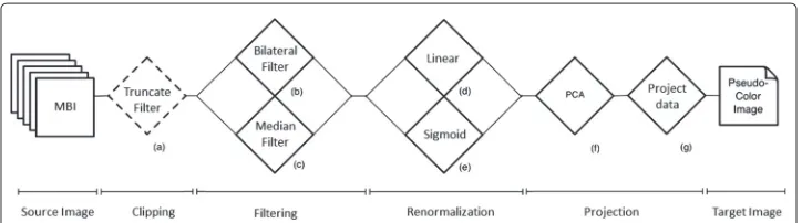
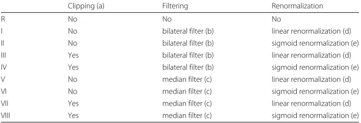
In this paper, we investigate eight different normalization protocols (I-VIII) and the raw intensity MBI (protocol R), as described in the remainder of this section. Figure 1 shows a unified workflow of the normalization pipeline for MBI, for all the eight protocols. The dashed boxes show optional processing modules and the solid boxes show mandatory process in the pipeline. Using different combination of these methods, we established and compared all the protocols as denoted in Table 1.

For the remainder of this paper, the following notation is used. LetDdenote the domain, for example the set of possible 12-bit intensities that can be measured in a single pixel pfor a single tagt. The width and height in pixels of an image are denoted bywandh respectively. So the set of all conceivable images for a single tag isDw×h_{. LetI}

t ∈ Dw×h

denote the intensity image corresponding to the tagtin a given MBI stack, and the entire stack consisting of images acquired usingNtags be denoted byIt∈Dw×h

t=1,...,N. We

denote byft(p)the intensity of pixel locationpin imageIt.

The truncate filter (a)

We first describe the non-mandatory step of clipping or truncation in the normalization pipeline, as shown in Fig. 1. Most of the denoising algorithms assume the underlying noise to be a Gaussian distribution. However, during image acquisition various non-Gaussian signals with impulsive characteristics are added to the image at extreme ends of the image histogram, and these may affect any follow-up analysis. To eliminate the outlier values, we truncate the highest and lowest values per intensity image as recently proposed in [25]

ˆ

ft(p)= ⎧ ⎪ ⎨ ⎪ ⎩

f0.01

t , ifft(p) <ft0.01 f99.99

t , ifft(p) >ft99.99 ft(p), otherwise

(1)

withfx

t being thex-th percentile ofIt.

Bilateral filter (b)

For denoising purposes, we explored two popular options: relatively recent bilateral fil-tering and the more conventional median filfil-tering. Bilateral filter [27] uses a combination

Table 1Normalization protocols as combinations of clipping, filtering, and renormalization methods

Clipping (a) Filtering Renormalization

R No No No

I No bilateral filter (b) linear renormalization (d) II No bilateral filter (b) sigmoid renormalization (e) III Yes bilateral filter (b) linear renormalization (d) IV Yes bilateral filter (b) sigmoid renormalization (e) V No median filter (c) linear renormalization (d) VI No median filter (c) sigmoid renormalization (e) VII Yes median filter (c) linear renormalization (d) VIII Yes median filter (c) sigmoid renormalization (e)

of domain and range filters that give relatively large weight to the pixels of a window in close proximity to the center pixel (whose value is to be smoothed) and having a similar intensity, and relatively small weight for pixels that are at a distance and have different intensities. LetMb denote theMb×Mbwindow with the pixelpto be smoothed at the center of the window. Mathematically, the bilateral filter can be written as follows,

ˆ

ft(p)=

1 o(p)

p∈_Mb

ft(p)g(p,p)s(p,p)

g(p,p)=e− ||p−p||2

2σ2

d

s(p,p)=e−

||ft(p)−ft(p)||2 2σ2

r

o(p)= p∈_Mb

g(p,p)s(p,p)

(2)

We applied bilateral filter with parametersMb=3,σd=0.5 andσr =10 for this work.

Median filter (c)

The median filter [28] is a popular non-linear filter conventionally used in fluorescence microscopy images. It replaces the intensity value of the center pixel with the median of intensity values of a neighborhood window of the sizeMm×Mm. The median filter

has excellent noise-reduction capabilities with good edge preservation particularly in the presence of bipolar and unipolar impulse noise [28]. Mathematically, the median filter can be expressed as follows,

ˆ

ft(p)=median p∈Mm

f(p) (3)

where Mm is an Mm × Mm filter. In this work, we employed median filtering using Mm=3.

Linear renormalization (d)

Variable dynamic range in an image corresponding a particular tagt, due for example to different exposure times, may result in biased results. Linear renormalization can be applied to ensure that the dynamic range of each image in the MBI stack is the same.

ˆ

ft(p)=

ft(p)−ftmin

f_tmax−f_tmin (4)

Sigmoid renormalization (e)

The strong binding of a protein marker in a particular region may produce high intensity values in that region, rendering the weaker regions almost completely unidentified for analysis purposes due to their relatively weaker intensity. To ensure that weaker signals are enhanced without further enhancing the stronger signals, the hyperbolic tangent function (a scaled form of the sigmoid function commonly used as a neuronal activation function) can be applied to each intensity image [21].

ˆ

ft(p)=tanh

1 2f_tmeanft(p)

(5)

withf_tmeanbeing the mean value ofIt.

Principal component analysis (PCA) (f)

After the application of a normalization strategy - made up of clipping (optional), fil-tering, and renormalization steps - we obtain for each set of MBIs N transformed intensity images It∈Dw×h

t=1,...,N. We flatten each image to get column vectors

I_t∈D(w·h)×1_t=1,...,N. We then defineM∈D(w·h)×Nas a matrix consisting of N such col-umn vectors. We compute the principal componentei∈RN, regarding each row ofMas

a data point [29].

Project data (g)

Due to the numeric computation of eigenvectors (i.e., the principal components), the ori-entation (not to be confused with the direction, accounting for the variance, of course) of principal componentseimay be arbitrary and needs to be aligned to avoid inverted color

projections (see below). To ensure that they have a similar direction, we set

ei=

ei, ifei· 1>0

−ei, otherwise

(6)

After this,Mis multiplied by an(w.h)×3 matrix consisting of the first three principal components

η=M [e1,e2,e3] , whereη∈R(w.h)×3 (7)

whereηcan be transformed back toO∈ Dw×h×3, resulting in 3 images each having the same size as each of theNnormalized tag images. Thereafter,Ois used as an RGB color image after linearly scaling the intensity values in the R, G, and B channels to the domain

Kullback-Leibler (KL) divergence

For quantitative comparison of the normalization protocols we performed Agglomera-tive Hierarchical Clustering (AGHC) andk-means, on average protein expression profile corresponding to each cell in an MBI, to generate cell phenotypes corresponding to histologically normal and cancer samples as described in [19]. To measure the differ-ence between discrete probability distributions of cell phenotyping profile, we employ a symmetric Kullback-Leibler (KL) divergence [31] defined by

KL(P,Q)= 1 2

i∈X

(P(i)−Q(i))logP(i)

Q(i) (8)

wherePandQare discrete probability distributions on a finite setXof cell phenotypes in MBI data. According to definition, the KL divergence should be higher when comparing different classes (‘Normal vs Cancer’) whereas it should be low when comparing within the same class (‘Normal vs Normal’ and ‘Cancer vs Cancer’).

Results

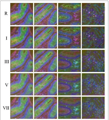
To minimize the effect of unknown variations in the data we start our analysis with four MBIs from the same patient, two each of cancerous and adjacent healthy tissue samples. We obtained pseudo-color (section ‘g’) visualizations using all the normalization proto-cols listed in Table 1 and requested two pathologists and two biologists to rank the results. The results for the top five protocols as ranked by the experts (Table 2) are shown in Fig. 2, whereas the results for the rest of normalization protocols have been added in Additional file 1: Figure A-1. The first two columns represent samples from histologically healthy colon tissue and the last two columns represent samples from cancerous tissue. Before the application of the normalization protocols defined above, the background fluores-cence signal was removed by subtracting the auto fluoresfluores-cence signal image just before applying the respective antibody tag. Two pathologists and two biologists were requested to rank the images based on the criteria A-C (see Materials and methods section above). The experts made following general observations on Fig. 2. Normalization protocols R & I show consistent blue color across the epithelial region in all the three cases where the epithelial cells are well organized around the crypt. Similarly, they shows greenish color inside the crypt and the stromal cells show the purple color in all the four cases. Normal-ization protocols III, V & VII show consistency in the normal cases but show different colors in the lumen and stromal regions for the cancer cases. Table 2 shows the rank of the normalization protocols as given by the two pathologists (A & B) and the two biolo-gists (C, & D). Three experts ranked normalization protocol I as consistently producing the best results, however one of the experts ranked it as the second best. The reason being that they seemed to be producing very similar results. When results from protocol I and

Table 2Rank given to normalization protocols R, I to VIII by two pathologists (A & B) and two biologists (C & D). The rows represent ranks given by each of the four experts whereas the columns represent rank of an MBI

Expert 1 2 3 4 5 6 7 8 9

A I R VII V III IV II VIII VI

B I R V II IV VII VIII VI III

C I R VII V III II IV VIII VI

Fig. 2Pseudocolor representation of normalization results. Column 1 to 4 represent four different cases: first two columns are from histologically normal tissue and the last two are from cancerous tissue of the same patient. Row 1 represents pseudo-color image obtained using raw pixel intensity values whereas row 2 to 5 represent psudo-color images obtained after applying different normalization protocols. See the text for details about results shown in I, III, V, VII. The pseudo-color images for the remaining normalization protocols are added in the Additional file 1: Appendix in Figure A-1

protocols show a variation in color in the epithelial cells around the crypt. Even in the healthy cases, the colors are not stable and show a lot of variation. The same is the true for the lumen areas, goblet cells and the stromal cells.

Another interesting feature of protocol R & I is the particular foreground / background contrast of one specific cell, which can be seen in the upper-left quadrant of images in the first column (Fig. 2). It appears as a small blue / cyan dot. An in-depth analysis has shown that this cell expresses an unusual combination of almost all proteins tagged in this exper-iment. Such rare occurrences could yield potential cues to rare events in the specimen, such as cancer stem cells. The contrast of this particular cell is high for protocols R, I, III, and V and ideal for protocol I and R.

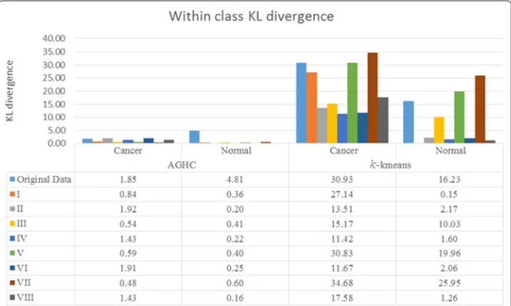
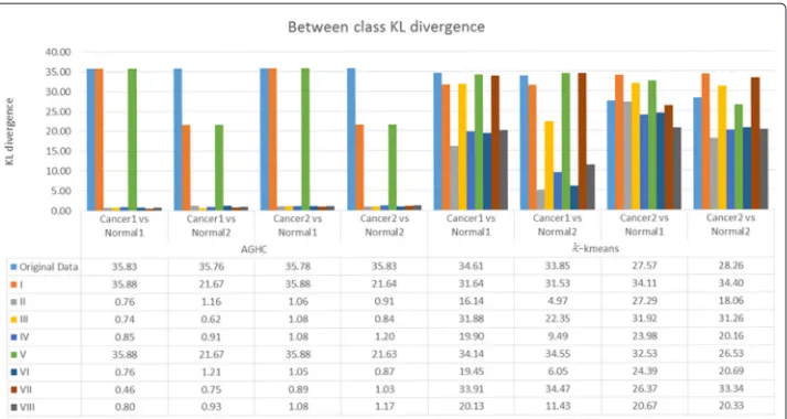
To compute KL divergence, distribution of cell phenotypes obtained using the method proposed in [19] was compared in normal and cancer samples. Figure 3 shows results for within class KL divergence, whereas Fig. 4 shows between class KL divergence results for normal and cancer samples, where Normal1 and Normal2 correspond to columns 1 and 2, whereas Cancer1 and Cancer2 refer to columns 3 and 4 respectively in Fig. 2. We expect lower within class KL-divergence as the same class should exhibit similar phenotypes whereas higher between class KL-divergence as different classes should exhibit different phenotypes. Figure 4 shows that only R, I and V produced higher KL divergence whereas the rest of the normalization protocols failed to show separation between the phenotypes while performing AGHC. Protocol R shows higher KL divergence in both Normal2 vs Cancer1 and Normal2 vs Cancer2 cases compared to protocol I and V which is desired, but it also shows higher within class KL divergence for Normal when performing AGHC. When Normal2 is carefully observed in Fig. 2, the stromal cells show a variation in colour within the same image for protocol R as can be seen in the stromal cell at the bottom of the image (Row 1, Column 2). Protocol I and V do not suffer from this discrepancy. Similarly, within class KL-divergence fork-means show higher values for protocol R & V.

Fig. 4Between class KL divergence after applying different normalization protocols. Only R, I & VII show higher KL divergence while performing AGHC &k-means

Compared to protocol R normalization protocol I shows lower within class KL divergence in allk-means cases. However, normalization protocol I shows higher KL divergence com-pared to II,III, IV, VI, VIII normalization protocols while performing phenotyping using k-means clustering on cancer data. This is likely due to the difference in histologic grade of the cancer tissues. The normal tissues on the other hand show very low KL divergence for protocol I. Protocol I shows higher KL divergence for all the cases except fork-means Cancer1 vs Normal1 and Cancer1 vs Normal2, but these values are very close to the ones obtained using protocol R. Protocol R on the other hand shows lower values for KL diver-gence for thek-means Cancer2 vs Normal1 and Cancer2 vs Normal2. Results obtained using protocol VII and IV can be studied in a meaningful way when the results from these protocols are combined in Figs. 3 and 4. Protocol VII shows higher between class KL divergence but it also shows higher KL divergence for within class KL divergence in Fig. 3. Similarly, protocol IV shows lower values in Fig. 3 but it also lowers the between class KL divergence.

We performed the same experiment with three MBIs collected from another patient, which contains one MBI from cancer sample and two MBIs from adjacent histologically normal samples. We have added the results in the Additional file 1: Appendix for within class KL-divergence in Additional file 1: Figure A-2 and for between class KL divergence in Additional file 1: Figure A-3. The KL-divergence result show similar kind of pattern for protocols R, I & V as in Figs. 3 and 4 respectively. The protocol R shows higher within class KL-divergence for normal samples withk-means clustering. However, for this patient, protocol VII behaved differently and shows higher between class KL-divergence when performing clustering using AGHC, but between class KL-divergence is lower for protocol VII when performing clustering usingk-means, showing inconsistency in the results.

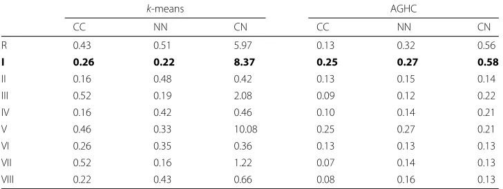
MBIs and a ‘cancer’ MBI mosaic using four cancer MBIs and perform clustering to obtain cell phenotypes. For between class KL-divergence, i.e., normal vs normal (NN) and cancer vs cancer (CC), we generate the mosaic by dividing each MBI into two halves and use one half to contribute to artificially generated one mosaic and the other half artificially generated second mosaic. In this way we can make sure that we are not missing any cell phenotypes which might be present in one patient and not in another. At the same time, by using half of the image we create separation between the data in a way that the data is not taken from the same region. The results for KL-divergence are shown in Table 3, which shows that protocol I shows lower within class KL-divergence and higher between class KL-divergence. In the case ofk-means protocol V shows higher between class KL-divergence but at the same time it has higher within class KL-KL-divergence. Also, for in the AGHC case, protocol V produces lower between class KL-divergence. Therefore, there is inconsistency in the results as evident from results in Fig. 3 and Additional file 1: Figure A-2 which shows higher within class KL-divergence for protocol V. Similarly, protocol R shows higher within class KL-divergence fork-means Normal case both in Fig. 3 and Additional file 1: Figure A-2. Normalization protocol I as ranked by majority of the experts increases the separation between clusters when comparing different classes but decreases this separation within the same class. The consistency of protocol I makes it the best choice for normalization among the comparable schemes.

Conclusions

Standardization of normalization procedures for data acquired from multiplexed bioimaging (MBI) technologies is as important as the standardization of protocols for the preparation of the tissue. This is mainly because of the presence of inherent limitations of the imaging apparatus, which can be due to variations in quality, quantity, or concen-tration of the antibody tag, exposure times, and quality of the camera and the microscope being used. Although efforts are being made to optimize the procedure for data acquisi-tion and preparaacquisi-tion of slides under the microscope [23], normalizaacquisi-tion of the data, i.e. the alignment of signals will always be necessary to overcome the variation across vari-ous runs for different types of tissue. Normalization protocols have been attempted in the past for other multiplexed technologies such as MALDI, mainly based on heuristics [24]. We presented a normalization pipeline for the normalization of MBI data and compared

Table 3KL-divergence result for the mosaic image created using multiple MBIs

k-means AGHC

CC NN CN CC NN CN

R 0.43 0.51 5.97 0.13 0.32 0.56

I 0.26 0.22 8.37 0.25 0.27 0.58

II 0.16 0.48 0.42 0.13 0.15 0.14

III 0.52 0.19 2.08 0.09 0.12 0.22

IV 0.16 0.42 0.46 0.10 0.14 0.21

V 0.46 0.33 10.08 0.25 0.27 0.21

VI 0.26 0.35 0.36 0.13 0.13 0.13

VII 0.52 0.16 1.22 0.07 0.14 0.13

VIII 0.22 0.43 0.66 0.08 0.16 0.13

the performance of its eight variants for data sets collected from ten different tissue sam-ples, six histologically healthy and four cancerous samples. Three of the four experts, two pathologists and two biologists, agreed on the normalization protocol I (made up of bilat-eral filtering followed by linear scaling) to be performing the best, whereas one expert ranked protocol I to be second best.

Protocol I also ranks best in terms of consistency in KL-divergence results, and is a combination of no clipping, bilateral filtering and linear normalization. Using protocol I, different constituents in the tissue, for example epithelial tissue, lumen and stromal cells produced consistent visualization across all the images from different types of tissue. In addition, normal and cancer tissues produced desired results after calculating KL diver-gence on cell phenotypes. The results suggest that if images do not contain over saturated intensities, clipping may destroy the quality of the data in those images. Bilateral filtering denoises the images but does not merge different compartments of the tissue as does the conventional median filtering. Linear scaling linearly stretches the intensities from 0 to 1 (maximum intensity), for all the protein expressions, therefore dynamic range of expres-sion of protein intensities is preserved across different runs, while the results suggest that non-linear sigmoid scaling degrades the quality of data. It seems that linear scaling has major impact on the normalization protocol as R, I, III, V & VII rank best by expert markings but if the results are studied in detail it is the combination of bilateral + lin-ear normalization which makes it the best normalization protocol. If bilateral filtering is replaced with median as in protocol V (No clipping + median + linear), protocol V shows different visualization for stromal cells in Fig. 2, in addition the results show higher within class KL-divergence in Fig. 3 and Additional file 1: Figure A-2. This suggests that it is the combination of No clipping + bilateral filtering + linear scaling which produces the best results.

Additional file

Additional file 1: Appendix.FigureA-1: Column 1 to 4 represent four different cases: first two columns are from histologically normal tissue and the last two are from cancerous tissue of the same patient. Rows 1 to 4 represent pseudo-color images obtained after applying low rank normalization protocols as marked by the experts. FigureA-2: Within class KL-divergence for Patient 2. Within class KL-divergence for second patient after performing phenotyping using different normalization protocols. FigureA-3: Between class KL-divergence for Patient 2. Between class KL-divergence for second patient after performing phenotyping using different normalization protocols. (PDF 341 kb)

Abbreviations

TIS: toponome imaging system; MBI: multiplexed bioimaging data; KL: Kullback-Leibler, CMP: combinatorial molecular patterns.

Competing interests

The authors declare that they have no competing interests.

Authors’ contributions

The manuscript was written through contributions of all authors. All authors have given approval to the final version of the manuscript. SEAR, DL, TN and NMR designed the study. SEAR, DL and KS performed the experiments.

Acknowledgements

The authors would like to thank David Snead, Hesham Eldaly, Yee-Wah Tsang, Stella Pelengaris and Linda Cheung for ranking the images for comparison of normalization strategies. The authors would also like to thank Sylvie Abouna and Michael Khan for help in collecting the data. We are grateful to the UK BBSRC and the Qatar National Research Fund (QNRF) for partially supporting this study through project grants BB/K018868/1 and NPRP 5-1345-1-228, respectively.

Author details

1_{Department of Computer Science, University of Warwick, CV4 7AL Coventry, UK.}2_{Biodata Mining Group, Bielefeld}

Received: 17 August 2015 Accepted: 2 February 2016

References

1. Evans RG, Naidu B, Rajpoot NM, Epstein D, Khan M. Toponome imaging system: multiplex biomarkers in oncology. Trends Mol Med. 2012;18(12):723–31.

2. Schubert W, Bonnekoh B, Pommer AJ, Philipsen L, Böckelmann R, Malykh Y, et al. Analyzing proteome topology and function by automated multidimensional fluorescence microscopy. Nat Biotechnol. 2006;24(10):1270–8. 3. Gerdes MJ, Sevinsky CJ, Sood A, Adak S, Bello MO, Bordwell A, et al. Highly multiplexed single-cell analysis of

formalin-fixed, paraffin-embedded cancer tissue. Proc Natl Acad Sci. 2013;110(29):11982–7.

4. Clarke GM, Zubovits JT, Shaikh Ka, Wang D, Dinn SR, Corwin AD, et al. A novel, automated technology for multiplex biomarker imaging and application to breast cancer. Histopathology. 2013;64(2):242–55.

5. Stoeckli M, Chaurand P, Hallahan DE, Caprioli RM. Imaging mass spectrometry: a new technology for the analysis of protein expression in mammalian tissues. Nat Med. 2001;7(4):493–6.

6. Giesen C, Wang HaO, Schapiro D, Zivanovic N, Jacobs A, Hattendorf B, et al. Highly multiplexed imaging of tumor tissues with subcellular resolution by mass cytometry. Nat Methods. 2014;11:417–22.

7. Bandura DR, Baranov VI, Ornatsky OI, Antonov A, Kinach R, Lou X, et al. Mass cytometry: technique for real time single cell multitarget immunoassay based on inductively coupled plasma time-of-flight mass spectrometry. Anal Chem. 2009;81(16):6813–22.

8. Van Manen HJ, Kraan YM, Roos D, Otto C. Single-cell Raman and fluorescence microscopy reveal the association of lipid bodies with phagosomes in leukocytes. Proc Natl Acad Sci of the U S A. 2005;102(29):10159–64.

9. Angelo M, Bendall SC, Finck R, Hale MB, Hitzman C, Borowsky AD, et al. Multiplexed ion beam imaging of human breast tumors. Nat Med. 2014;20:.

10. Goodwin RJa. Sample preparation for mass spectrometry imaging: small mistakes can lead to big consequences. J Proteome. 2012;75(16):4893–911.

11. Schubert W, Gieseler A, Krusche A, Serocka P, Hillert R. Next-generation biomarkers based on 100-parameter functional super-resolution microscopy TIS. New Biotechnol. 2012;29(5):599–610.

12. Bode M, Krusche A. Toponome Imaging System (TIS): imaging the proteome with functional resolution. Nat Methods Appl Notes. 2007;4:1–2.

13. Friedenberger M, Bode M, Krusche A, Schubert W. Fluorescence detection of protein clusters in individual cells and tissue sections by using toponome imaging system: sample preparation and measuring procedures. Nat Protoc. 2007;2(9):2285–94.

14. Raza SEA, Humayun A, Abouna S, Nattkemper TW, Epstein DBA, Khan M, et al. RAMTaB: robust alignment of multi-tag bioimages. PLoS ONE. 2012;7(2):e30894.

15. Nattkemper TW, Ritter HJ, Schubert W. A neural classifier enabling high-throughput topological analysis of lymphocytes in tissue sections. Inf Technol Biomed IEEE Trans. 2001;5(2):138–149.

16. Nattkemper TW, Wersing H, Schubert W, Ritter H. A neural network architecture for automatic segmentation of fluorescence micrographs. Neurocomputing. 2002;48(1–4):357–67.

17. Schubert W, Friedenberger M, Haars R, Bode M, Philipsen L, Nattkemper T, et al. Automatic recognition of muscle-invasive t-lymphocytes expressing Dipeptidyl-Peptidase IV (CD26) and analysis of the associated cell surface phenotypes. J Theoretical Med. 2002;4(1):67–74.

18. Herold J, Schubert W, Nattkemper TW. Automated detection and quantification of fluorescently labeled synapses in murine brain tissue sections for high throughput applications. J Biotechnol. 2010;149(4):299–309.

19. Khan AM, Raza SEA, Khanm M, Rajpoot NM. Cell phenotyping in multi-tag fluorescent bioimages. Neurocomputing. 2014;134:254–61.

20. Loyek C, Rajpoot NM, Khan M, Nattkemper TW. BioIMAX: A Web 2.0 approach for easy exploratory and collaborative access to multivariate bioimage data. BMC Bioinformatics. 2011;12(1):297.

21. Kölling J, Langenkämper D, Abouna S, Khan M, Nattkemper TW. WHIDE–a web tool for visual data mining colocation patterns in multivariate bioimages. Bioinformatics (Oxford, England). 2012;28(8):1143–50.

22. Kovacheva VN, Khan AM, Khan M, Epstein D, Rajpoot NM. DiSWOP: a novel measure for cell-level protein network analysis in localised proteomics image data. Bioinformatics. 2014;30(3):420–7.

23. Linke B, Pierre S, Coste O, Angioni C, Becker W, Maier TJ, et al. Toponomics analysis of drug-induced changes in arachidonic acid-dependent signaling pathways during spinal nociceptive processing. J Proteome Res. 2009;8(10): 4851–9.

24. Fonville JM, Carter C, Cloarec O, Nicholson JK, Lindon JC, Bunch J, et al. Robust data processing and normalization strategy for MALDI mass spectrometric imaging. Anal Chem. 2012;84(3):1310–9.

25. Schüffler PJ, Schapiro D, Giesen C, Wang HaO, Bodenmiller B, Buhmann JM. Automatic single cell segmentation on highly multiplexed tissue images. Cytometry Part A. 2015;87(10):936–42.

26. Bhattacharya S, Mathew G, Ruban E, Epstein DBA, Krusche A, Hillert R, et al. Toponome Imaging System : in situ protein network mapping in normal and cancerous Colon from the same patient reveals more than five-thousand cancer specific protein clusters and their subcellular annotation by using a three symbol code research articles. J Proteome Res. 2010;9(12):6112–25.

27. Tomasi C, Manduchi R. Bilateral filtering for gray and color images. In: Sixth International Conference on Computer Vision (IEEE Cat. No.98CH36271). Bombay: IEEE; 1998. p. 839–46.

28. González RC, Woods RE. Digital image processing. USA: Pearson/Prentice Hall; 2008.

29. Bishop CM. Pattern. Pattern Recognition and Machine Learning In: Jordan M, Kleinberg J, Schölkopf B, editors. Information Science and Statistics. 1st ed. Berlin Heidelberg: Springer; 2006. p. 738.

30. Herold J, Loyek C, Nattkemper TW. Multivariate image mining. Wiley Interdiscip Rev Data Mining Knowl Discov. 2011;1(1):2–13.