A stability analysis of thermostatically controlled loads for power system frequency control

warwick.ac.uk/lib-publications

Original citation:

Webborn, Ellen and MacKay, R. S. (Robert Sinclair) (2017) A stability analysis of

thermostatically-controlled loads for power system frequency control. Complexity, 2017.

5031505. doi:10.1155/2017/5031505

Permanent WRAP URL:

http://wrap.warwick.ac.uk/93213

Copyright and reuse:

The Warwick Research Archive Portal (WRAP) makes this work of researchers of the

University of Warwick available open access under the following conditions.

This article is made available under the Creative Commons Attribution 4.0 International

license (CC BY 4.0) and may be reused according to the conditions of the license. For more

details see:

http://creativecommons.org/licenses/by/4.0/

A note on versions:

The version presented in WRAP is the published version, or, version of record, and may be

cited as it appears here.

Research Article

A Stability Analysis of Thermostatically Controlled Loads for

Power System Frequency Control

Ellen Webborn

and Robert S. MacKay

1_{Centre for Complexity Science, University of Warwick, Coventry, UK}

2_{Mathematics Institute, University of Warwick, Coventry, UK}

Correspondence should be addressed to Ellen Webborn; [email protected]

Received 30 June 2017; Accepted 10 October 2017; Published 6 December 2017

Academic Editor: Paul Hines

Copyright © 2017 Ellen Webborn and Robert S. MacKay. This is an open access article distributed under the Creative Commons Attribution License, which permits unrestricted use, distribution, and reproduction in any medium, provided the original work is properly cited.

Thermostatically controlled loads (TCLs) are a flexible demand resource with the potential to play a significant role in supporting electricity grid operation. We model a large number of identical TCLs acting autonomously according to a deterministic control scheme to provide frequency response as a population of coupled oscillators. We perform stability analysis to explore the danger of the TCL temperature cycles synchronising: an emergent phenomenon often found in populations of coupled oscillators and predicted in this type of demand response scheme. We take identical TCLs as it can be assumed to be the worst case. We find that the uniform equilibrium is stable and the fully synchronised periodic cycle is unstable, suggesting that synchronisation might not be as serious a danger as feared. Then detailed simulations are performed to study the effects of a population of frequency-sensitive TCLs acting under real system conditions using historic system data. The potential reduction in frequency response services required from other providers is determined, for both homogeneous and heterogeneous populations. For homogeneous populations, we find significant synchronisation, but very minimal diversity removes the synchronisation effects. In summary, we combine dynamical systems stability analysis with large-scale simulations to offer new insights into TCL switching behaviour.

1. Introduction

To operate the electricity grid reliably and securely requires controlling a number of factors, one of which is the electricity grid frequency. The AC frequency continually varies close to its nominal value (50 Hz in Europe) and is kept there by the System Operator (SO) in order to respect regulations and prevent network instabilities and blackouts. This is mainly done by employing flexible power generators, such as gas turbines, to vary their output in response to imbalance between supply and demand. This type of service is often known as frequency response, or frequency regulation. With the arrival of large numbers of wind and solar farms, smart meters, and thousands of domestic solar panels, uncontrolled and largely invisible to the System Operator, new challenges and opportunities have arisen. Rather than relying on a few large (typically fossil-fuelled) power plants to provide system balancing, there is the potential, and perhaps a need, for consumers to play a role. However, for a large number of

very small players to participate would require a modelling approach capable of incorporating the complexities of such a system and foreseeing emergent phenomena that may arise as a result of the interactions involved. In this article we explore the potential for certain types of domestic appliances to provide frequency response through simple deterministic rules and consider the possibility of (potentially harmful) demand synchronisation.

Thermostatically controlled loads (TCLs) are well-suited for the provision of demand-side response (DSR), due to their simple temperature set point operating rules and ubiquity in society. Examples include fridges, freezers, air-conditioners, hot-water tanks, heat pumps, and swimming pool pumps. Research into the possibility of using TCLs for grid balancing services began in the 1980s with key papers such as [1–4]. Despite the existence of technology for creating frequency-sensitive TCLs for nearly 40 years, implementation remains limited to a relatively small number of trials [5–9]. There are a number of reasons for the absence of large roll-outs of

Table 1: Comparison of centralised and decentralised TCL control strategies. Informed by, for example, [19, 38].

Centralised control Decentralised control

Key features

(i) TCLs instructed by a central controller (i) Autonomous local control

(ii) 2-way communication in all TCLs (ii) Control scheme established once, may be updated periodically

Advantages

(i) Highly controllable (i) No communications infrastructure

required

(ii) Reasonably predictable (ii) No security risks

(iii) Very fast response possible

Disadvantages

(i) Establishing and maintaining a secure communications network are very expensive

(ii) Response time limited by communication speed

(iii) Vast amounts of data to manage (iv) Data and appliance control security risks

(v) Negative public perceptions of external control of home appliances

(i) Response is less predictable than with centralised control

(ii) Synchronisation and instability effects possible and not yet fully understood (iii) Errors and noise in local frequency measurements more likely

highly distributed DSR schemes [10, 11]. Historically, control paradigms from both technical and economic perspectives have been established for service provision from a (relatively) small number of large power plants. Understandably, the critical nature of electricity grid operation and security deters potentially risky changes and experimentation, and so a great deal of motivation is required for shifts away from traditional approaches. Service availability and reliability can be improved by splitting a service between a multitude of providers, compared to a single unit which will become completely unavailable in the event of a fault or scheduled repair [9, 12]. Yet there is also inherent complexity and potentially reduced predictability in procuring services from thousands of very small demand-side resources if they act autonomously, which is undoubtedly an obstacle to be overcome. Effects on consumers and their appliances will also be of concern to potential participants. Finally, it will be crucial for the success of any scheme, to adequately address the requirements for minimum participation numbers and develop the right business models that ensure fair rewards and effective incentives.

The changing energy landscape in the 21st century has brought a new focus to the use of TCLs for electricity grid support and a wealth of literature on the topic [5, 9–11, 13–37]. Work has varied in nature from mathematical frameworks to numerical simulations and real-world trials. Most of the theory can be applied to any type of TCL, and simulations have covered many different possible TCL technologies. A variety of control schemes have been proposed, many of which are discussed and compared in [10, 19, 35]. There are two main classes into which these types of TCL control schemes can be divided:centralised and decentralised con-trol (with a spectrum in between). Their key features and comparative advantages and disadvantages are summarised in Table 1. It is widely accepted that if millions of TCLs could be used for frequency response they could potentially provide a valuable resource for the system. However, if each device

needed constant communication with a central controller, sending data about its temperature and switching history and receiving operation instructions, then the economics and security risks would severely outweigh the benefits of the service. Public perception of the service is also vital for the implementation of any control scheme that involves appliances in people’s homes. For these reasons we choose to focus on decentralised control for our research. A better understanding, however, of the potential undesirable side-effects of decentralised control, is required before any control strategy could be put in place.

randomly switch on and off could cause negative public perceptions of a DSR scheme. We believe further study of potential deterministic schemes would be beneficial before putting attention on stochastic schemes, particularly given the natural diversity in TCL populations that could prevent synchronisation phenomena.

An alternative to direct instructions and frequency sig-nals is the use of a price signal that TCLs could respond to. The advantages of price signals are that it is possible to measure the financial benefits to consumers of DSR participation, and individual consumers could potentially make their own choices about the value they place on service disruption at, say, given times of day. However, current price signals typically change on half-hourly or at least several-minute time scales, which makes them ill-suited for dynamic frequency response. Reviews on the use of price signals for demand response can be found in [41–43]. A related approach proposed in [44] involves each device calculating the price directly from the grid frequency, and the authors argue that a well-chosen design for the controller and frequency-price coupling may prevent possible oscillations and instabilities. However, the drawbacks of price-based demand response, as remarked upon in [27], are the potential for synchronisation and the exposure of customers to price volatility, which could prevent sufficient participation for success.

In [13] Angeli and Kountouriotis offer theoretical argu-ments for the long-term tendency of the system towards TCL synchronisation. It is reasoned that any “small periodic ripples in power system frequency will gradually entrain oscillations of refrigerators that have similar frequencies of oscillation, thus reinforcing the frequency ripple and eventually leading to an even larger number of entrained refrigerators.” We concur with the mathematical reasoning presented. However, we believe that further reasoning and inquiry are required for a more complete understanding of this phenomenon.

A population of TCLs responding to frequency through preset deterministic rules with no other communications or control can be thought of as a system of coupled oscil-lators. Synchronisation phenomena emerging from systems of coupled oscillators have been studied in many contexts, from neural signals in the brain to flashing fireflies [45]. The Kuramoto framework was developed [46, 47] which elegantly describes basic features of such systems and allows for stability analysis. Inspired by results for the Kuramoto model, in this article we explore the stability of a system of TCLs and grid frequency using techniques from dynamical systems and agent-based modelling.

We study the potential for a population of TCLs to support grid frequency and explore the possibilities for frequency-sensitive TCLs to cause instabilities due to cycle synchronisation. We use techniques from dynamical systems stability analysis along with simulations that incorporate data from the British power grid. In Section 2 we introduce our model for a population of TCLs and the electricity grid frequency and explain our choices of parameter values. In Section 3.1 we present a stability analysis of the nominal frequency in the presence of a uniformly distributed pop-ulation of TCLs. Section 3.2 solves the behaviour of a fully

synchronised TCL population and analyses the stability of the population under a split into two groups. Section 4.1 describes our simulations of a large population of TCLs using the model in Section 3.1. Section 4.2 describes our simulations of a population of TCLs acting on the system in the presence of other frequency response providers and naturally occurring frequency fluctuations, including simulations of a heteroge-neous population. Section 5 contains our final discussion and conclusions.

2. Modelling TCLs and Electricity

Grid Frequency

The modelling is kept appliance-neutral where possible, but it is set up for cooling devices such as fridges, (fridge-)freezers, and air-conditioners and would need to be altered in minor ways for other appliances such as heat pumps and hot-water tanks. We make the following assumptions:

(i) Electricity grid frequency is the same everywhere on the network and there are no inter-area oscillations [48] (therefore all machines on the power grid are assumed to rotate in synchrony).

(ii) All TCLs sense frequency deviations with negligible measurement delay or measurement error.

(iii) All system parameters remain constant over time. (iv) Fridges and freezers are not affected by the fridge/

freezer door being opened, or by the addition or removal of food (in effect we assume this never occurs).

(v) TCLs have continuous thermostat control (in temper-ature and time) and can therefore sense and imple-ment temperature/set point changes with infinite precision.

(vi) TCLs consume constant power when on and zero power when off and are controlled only by the rules outlined in the model.

These assumptions allow us to create a tractable model for analytic study. Assumptions (iii) and (iv) are probably the easiest and most natural to relax first and could be relaxed by adding time-dependent forcing effects. For most of the paper we consider a population of identical TCLs, but our formulation can be extended easily to an inhomogeneous population and we believe the effects of sufficient diversity will be stabilising, as supported by our final simulation.

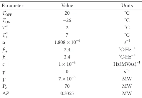
2.1. Individual TCLs. For the temperature cycling of a TCL we adopt the linear model and notation presented in [13]. Let the temperature of a TCL at time𝑡be denoted by𝑇(𝑡), the cooling/heating coefficient by 𝛼, and the asymptotic temperatures that the TCL would reach if left on and off indefinitely by𝑇_ONand𝑇_OFF, respectively. Then

̇𝑇 (𝑡) ={_{ {

𝛼 (𝑇ON− 𝑇 (𝑡)) when the TCL is on 𝛼 (𝑇OFF− 𝑇 (𝑡)) when the TCL is off.

A (cooling) TCL will switch off when the temperature reaches its lower temperature set point 𝑇₋ and switch on when it reaches its upper temperature set point𝑇₊. We choose to make these set points sensitive to system frequency deviations away from 50 Hz, denoted𝑓(𝑡)(i.e.,𝑓(𝑡) =Frequency(𝑡) −

50Hz). Insufficient generation to meet demand causes𝑓 < 0 and so we need the TCLs to reduce their power consumption to bring𝑓back to zero. We implement this by increasing the temperature set points so that the TCLs switch off sooner/stay off for longer. Oversupply of electricity to the grid causes

𝑓 > 0, and so in this case we decrease the temperature set points to increase overall power consumption. Thus we define our frequency-sensitive temperature set points,

𝑇₋(𝑓 (𝑡))fl𝑇₋0− 𝛽₋𝑓 (𝑡)

lower(switch off)set point (2a)

𝑇₊(𝑓 (𝑡))fl𝑇₊0− 𝛽₊𝑓 (𝑡)

upper(switch on)set point, (2b)

where 𝛽₋, 𝛽₊ are positive constants that determine the sensitivity of the lower and upper temperature set points to frequency deviations.𝑇₋0and𝑇₊0are the uncoupled (a fridge is “uncoupled” from the grid frequency if 𝛽₋ = 𝛽₊ = 0) temperature set points, which we typically take to be 2∘C and7∘C, respectively. This framework is very similar to that suggested in [30], although we allow the upper and lower temperature set points to have different sensitivities to the frequency (𝛽₋and𝛽₊).

We can solve (1) for the temperature of a TCL at time𝑡. If a TCL has temperature𝑇₀at time𝑡₀and does not switch on or off before time𝑡then the temperature𝑇(𝑡)is given by

𝑇 (𝑡) = (𝑇0− 𝑇ON) 𝑒−𝛼(𝑡−𝑡0)+ 𝑇ON when on (3a)

𝑇 (𝑡) = (𝑇0− 𝑇OFF) 𝑒−𝛼(𝑡−𝑡0)+ 𝑇OFF when off. (3b)

We can rearrange (3a) and (3b) and solve for the on and off durations𝜏_ONand𝜏_OFF, respectively, assuming constant grid frequency:

𝜏_ON(𝑓) = 1 𝛼log(

𝑇+(𝑓) − 𝑇ON

𝑇₋(𝑓) − 𝑇_ON) (4a)

𝜏OFF(𝑓) = 1 𝛼log(

𝑇_OFF− 𝑇₋(𝑓)

𝑇OFF− 𝑇+(𝑓)) . (4b)

These variables will be useful when we consider the equi-librium of the system, in which the temperature set points become fixed. In the traditional case when TCLs are uncou-pled from the grid (or the special case𝑓 ≡ 0) their “natural” on and off cycle durations,𝜏_ON0 and𝜏_OFF0 , are given by

𝜏_ON0 = 1 𝛼log(

𝑇0

+− 𝑇ON

𝑇0

−− 𝑇ON

) (5a)

𝜏_OFF0 = 1 𝛼log(

𝑇OFF− 𝑇−0

𝑇OFF− 𝑇+0) .

(5b)

In order for the TCLs to operate properly they need to cycle on and off, and so we require that

𝑇ON< 𝑇−(𝑓 (𝑡)) < 𝑇+(𝑓 (𝑡)) < 𝑇OFF ∀𝑡. (6)

We also need a TCL to respond “appropriately” to a change in frequency, that is to say, for the average power consumption over one cycle to increase when the frequency increases and decrease when the frequency decreases. It is shown in Appendix A that a sufficient condition to ensure this is

𝛽₊ 𝛽₋ ∈ (

𝑇_OFF− 𝑇₊ 𝑇OFF− 𝑇−,

𝑇₊− 𝑇_ON 𝑇₋− 𝑇ON

) (7)

which is a nonempty interval (notably containing{1}).

2.2. Electricity Grid Frequency. A simplified equation for the frequency 𝐹 of a power system can be determined by Newton’s 2nd Law of Motion or the derived equation for energy. If we let𝑓 fl 𝐹 − 𝐹₀, where𝐹₀is the nominal grid frequency (50 Hz in Europe) and linearise about𝐹₀, then we obtain [26]

𝑀d𝑓

d𝑡 + 𝐷𝑓 (𝑡) = Δ𝑃𝑔− Δ𝑃𝑙 (8)

and for brevity we introduce new variables along with explicit consideration of TCL power consumption

d𝑓

d𝑡 (𝑡) = 𝑐 (Δ𝑃 − 𝜌 (𝑡) 𝑃𝑐) − 𝛾𝑓 (𝑡) , (9)

where

𝑀 fl 4𝜋2_𝐼𝐹

0 stands for 2𝜋times nominal angular

momentum of the rotating masses in the system,

𝐼stands for total inertia of the rotating masses of the system,

𝐷stands for damping factor representing the natural frequency dependence of the load alongside the damping provided by synchronous generator damper windings,

Δ𝑃𝑔 stands for change in total active power

genera-tion, compared to a reference level,

Δ𝑃_𝑙 stands for change in total active power load, compared to a reference level,

𝑐fl1/𝑀stands for inverse nominal angular momen-tum, introduced for brevity,

Δ𝑃 stands for “surplus power generation for the TCLs;” total system active power generation minus total system active power load, excluding TCL power consumption,

𝜌stands for proportion of TCLs switched on,

𝑃_𝑐 stands for power consumed by TCL population when all switched on,

We make the simplifying assumption in Sections 2 and 3 that the “surplus” power generation on the system for TCL consumptionΔ𝑃is a constant. We use the “∗” notation to denote equilibrium values. In equilibrium

𝑐 (Δ𝑃 − 𝜌∗𝑃_𝑐) − 𝛾𝑓∗ = 0, (10)

hence

𝑓∗ ₌ 𝑐

𝛾(Δ𝑃 − 𝜌∗𝑃𝑐) , (11)

and therefore we can rewrite our equation for𝑓̇in terms of deviations from equilibrium values:

̇̃𝑓(𝑡) = 𝑐𝑃𝑐(𝜌∗− 𝜌 (𝑡)) − 𝛾 ̃𝑓, (12)

where

̃

𝑓fl𝑓 − 𝑓∗. (13)

2.3. Parameter Choices. We take as reference the Great Britain (GB) electricity system. This covers England, Scotland, and Wales. In 2015 approximately 10.4 m households in the UK, which also includes Northern Ireland, owned a fridge and 19.1 m households owned a fridge-freezer [49]. In the same year approximately 2.8% of the population lived in Northern Ireland [50]. If we assume that the average number of people per household is the same in Northern Ireland and in GB and an even distribution of fridge and fridge-freezer ownership, then approximately 10.1 m and 18.6 m households in GB owned a fridge and fridge-freezer, respectively. If using TCLs for frequency response became standard practice, that would mean that a very large number of appliances could participate in frequency response. We model the case of 1 million fridges participating in frequency response, which corresponds to roughly10% of fridges in GB. We take the power consumed by an individual fridge when switched on,𝑝, to be 70 W, as assumed in [32, 33]. This means that we let𝑝 = 7 × 10−5MW and the total power consumption if all fridges were switched on,𝑃_𝑐= 7×10−5×106= 70MW. Using our approximation for

̇

𝑓(𝑡)[51],𝑐 = 50/(2𝐸_𝑘). Our GB system data (discussed later) gives an approximate average value for total stored kinetic energy𝐸_𝑘;𝐸_𝑘 = 2.5 × 105MVAs (note that MVAs = MJ), and so𝑐 = 1 × 10−4. We let 𝜌∗ vary between 0 and 1 by changingΔ𝑃. Our parameters are summarised in Table 2, and throughout this paper take these values unless stated otherwise.

3. Stability Analysis

Concerns that frequency-responsive TCLs controlled by deterministic rules will exhibit herding behaviour and create frequency oscillations have been raised in various previous works, either by predictions or examples from simulations [13, 21, 22, 25, 30–32]. The simplicity of our model allows for a rigorous mathematical treatment of the stability of a population of TCLs responding according to the scheme introduced above. In the first part of this section we model a TCL population as a continuum on the temperature cycle

Table 2: Parameter values assumed, unless stated otherwise.

Parameter Value Units

𝑇OFF 20 ∘C

𝑇_ON −26 ∘C

𝑇0

− 2 ∘C

𝑇0

+ 7 ∘C

𝛼 1.808 × 10−4 _s−1

𝛽₊ 2.4 ∘C⋅Hz−1

𝛽− 2.4 ∘C⋅Hz−1

𝑐 1 × 10−4 _Hz(MVAs)−1

𝛾 0 s−1

𝑝 7 × 10−5 _MW

𝑃_𝑐 70 MW

Δ𝑃 0.3355 MW

and linearise about the equilibrium discussed in Section 2.2. In the second part of this section we consider the opposite extreme for a TCL distribution (one or two Dirac delta distributions), solving for the behaviour of a fully synchro-nised population of TCLs and studying the dynamics of two synchronised groups.

3.1. Uniform Distribution of TCLs. We begin by studying the stability of a population of TCLs uniformly distributed in phase (meaning the time since last switch on). This means that under constant temperature set point conditions the TCLs would switch on at a constant rate and switch off at a (possibly different) constant rate (note that since TCLs heat (or cool) at different rates depending on their current temperature, uniformly distributing the TCLs within each part of the cycle does not correspond to uniformly distributing the population over the temperature scale). In the context of the Kuramoto model this is usually referred to as the “incoherent solution,” for example [47, 52]. Just as in Strogatz and Mirollo’s treatment of the Kuramoto model [52], we model the infinite-N limit of a population of TCLs as a continuum of TCLs distributed over an interval with periodic boundary conditions.

In order to obtain a tractable model, comparable to the Kuramoto model, three key challenges must be addressed. Firstly, the TCL temperature cycling is described by the piecewise-smooth nonlinear function (see (3a) and (3b)), with nondifferentiability at each temperature set point. Sec-ondly, these set points are continuously changing with grid frequency, and so any map to a periodic regime must be sufficiently flexible to accommodate this. Finally, in order to know a TCL’s rate of change of temperature at any time, one needs to know both its current temperature and its current (on/off) state. We therefore propose a new modelling framework to overcome these challenges and permit stability analysis for the model.

𝜃(𝑡)of a TCL at time𝑡with temperature𝑇(𝑡)and state on or off by

𝜃 (𝑡) = { { { { { { { { {

𝜃ON(𝑡) = 1

𝛼𝜏_ON(𝑓 (𝑡))log(

𝑇+(𝑓 (𝑡)) − 𝑇ON

𝑇 (𝑡) − 𝑇ON ) ∈ [0, 1)

if on

𝜃OFF(𝑡) = 1

𝛼𝜏_OFF(𝑓 (𝑡))log(

𝑇OFF− 𝑇+(𝑓 (𝑡))

𝑇OFF− 𝑇 (𝑡) ) ∈ [−1, 0) if off.

(14)

Note that the model implicitly assumes that the temperature set points never change fast enough to leave a TCL outside of the interval[𝑇₋(𝑓(𝑡)), 𝑇₊(𝑓(𝑡))]. Since in this paper we use this model for only linear stability analysis about the equilib-rium, we consider this to be a reasonable assumption. Our choice of𝜃means that uniformly distributing a population of TCLs over each part of the temperature cycle (as discussed above) corresponds to a uniform distribution of on and off TCLs in their respective halves of𝜃-space.

As in [52], we consider the population density in𝜃-space; let𝑢(𝜃, 𝑡)d𝜃denote the fraction of TCLs that lie between𝜃 and𝜃+d𝜃at time𝑡. Then𝑢is nonnegative, with period length 2 in𝜃, and satisfies the normalisation

∫+1

−1 𝑢 (𝜃, 𝑡)d𝜃 = 1 (15)

for all 𝑡. The evolution of𝑢 is governed by the continuity equation [53]

𝜕𝑢 𝜕𝑡 +

𝜕

𝜕𝜃(𝑢V) = 0, (16)

whereVis the velocity of a TCL in𝜃-space,V(𝜃, 𝑡) fl ̇𝜃(𝑡). Differentiating (14) gives

VON(𝜃, 𝑡) = 1 𝜏ON(𝑓 (𝑡))

(1

+1_𝛼[𝜙ON(𝑓 (𝑡)) 𝜃 −

𝛽+

𝑇₊(𝑓 (𝑡)) − 𝑇ON

] ̇𝑓 (𝑡))

(17a)

VOFF(𝜃, 𝑡) = 1

𝜏_OFF(𝑓 (𝑡))(1

+1

𝛼[𝜙OFF(𝑓 (𝑡)) 𝜃 +

𝛽₊

𝑇OFF− 𝑇+(𝑓 (𝑡))] ̇𝑓 (𝑡)) ,

(17b)

where

𝜙ON(𝑓)fl

𝛽+

𝑇₊(𝑓) − 𝑇ON

− 𝛽−

𝑇₋(𝑓) − 𝑇ON

(18a)

𝜙OFF(𝑓)fl

𝛽₊ 𝑇_OFF− 𝑇₊(𝑓)−

𝛽₋

𝑇_OFF− 𝑇₋(𝑓). (18b)

Note that, for 𝛽₊/𝛽₋ satisfying (7), 𝜙_ON(𝑓) < 0 and

𝜙OFF(𝑓) > 0. Under a constant grid frequency, OṄ𝜃 and

̇𝜃

OFFare constants. In equilibrium𝑢∗ we have ̇𝑢∗ = 0, and therefore (16) implies

𝑢∗_ON(𝜃) = 𝑘0

V∗

ON(𝜃) ;

𝑢_OFF∗ (𝜃) =_V∗𝑘0 OFF(𝜃)

,

(19)

for some constant𝑘₀. Since𝑓∗̇ = 0, from (17a) and (17b) we have

V∗_ON= 1

𝜏∗

ON ;

V∗

OFF= 1 𝜏∗

OFF .

(20)

Then for all𝜃 ∈ [−1, 0), [0, 1), respectively,

𝑢∗_ON(𝜃) = 𝑘0𝜏ON∗ 𝑢∗_OFF(𝜃) = 𝑘0𝜏OFF∗

(21)

and𝑘₀is determined by the normalisation criterion (15),

𝑘₀= 1

𝜏∗

ON+ 𝜏OFF∗

. (22)

The proportion of TCLs switched on,𝜌(𝑡), is given by

𝜌 (𝑡) = ∫1

0 𝑢 (𝜃, 𝑡)d𝜃. (23)

In equilibrium𝜌(𝑡) = 𝜌∗(12),

𝜌∗= ∫1

0 𝑢

∗_{(𝜃, 𝑡)d𝜃 =} 𝜏ON∗ 𝜏∗

ON+ 𝜏OFF∗

. (24)

We introduce the notation “∙” to imply that an equation holds for the variable with either of two values, “on” or “off.” Our approach is to perturb the system about the equilibrium

(𝑢∗_{, 𝑓}∗_{)by a small amount𝜏}∗

∙𝜂(𝜃, 𝑡)and to consider the

evo-lution of the perturbation. By (15) the perturbation satisfies

∫+1

We write

𝑢∙= (𝑘0+ 𝜂 (𝜃, 𝑡)) 𝜏∙∗ (26)

V_∙= _𝜏1_∗

∙ (1 + 𝑤 (𝜃, 𝑡)) (27)

so that (16) becomes

𝜏_∙∗ 𝜕 𝜕𝑡[𝜂] +

𝜕

𝜕𝜃[𝑘0+ 𝑘0𝑤 + 𝜂 + 𝜂𝑤] = 0. (28)

Taking the first-order approximation yields

𝜏_∙∗ 𝜕

𝜕𝑡[𝜂] + 𝑘0 𝜕 𝜕𝜃[𝑤] +

𝜕

𝜕𝜃[𝜂] = 0. (29)

Rearranging (27) for𝑤and substituting (17a) and (17b) forV_∙ give

𝑤ON= 1

𝛼(𝜙∗ON𝜃 − 𝛽₊ 𝑇∗

+ − 𝑇ON

) ̇𝑓 (𝑡) −𝛿𝜏ON(𝑡) 𝜏∗

ON

𝑤OFF= 1

𝛼(𝜙∗OFF𝜃 + 𝛽₊

𝑇OFF− 𝑇+∗) ̇𝑓 (𝑡) −

𝛿𝜏OFF(𝑡) 𝜏∗

OFF ,

𝛿𝜏ON(𝑡) = − 𝜙∗

ON𝑓 (𝑡)̃

𝛼 ; 𝛿𝜏OFF(𝑡) = − 𝜙∗

OFF𝑓 (𝑡)̃

𝛼 .

(30a)

Hence

𝜕

𝜕𝜃[𝑤∙(𝑡)] = 1

𝛼[𝜙∗∙𝑓 + (𝑤 (𝑡)|̇ 𝜃=0+− 𝑤 (𝑡)|_𝜃=0−) 𝛿 (𝜃)

+ (𝑤 (𝑡)|𝜃=−1− 𝑤 (𝑡)|𝜃=1) 𝛿 (𝜃 − 1)]

𝜕

𝜕𝜃[𝑤∙(𝑡)] = 1

𝛼[𝜙∗∙𝑓 −̇ ]0𝛿 (𝜃) +]1𝛿 (𝜃 − 1)] ̇𝑓 (𝑡)

+𝜇

𝛼[𝛿 (𝜃 − 1) − 𝛿 (𝜃)] ̃𝑓,

(31)

where we have defined

]₀fl _𝑇∗𝛽+

+ − 𝑇ON

+_𝑇 𝛽+

OFF− 𝑇+∗ > 0 (32a)

]₁fl 𝛽−

𝑇∗

− − 𝑇ON

+ 𝛽−

𝑇OFF− 𝑇−∗ > 0 (32b)

𝜇fl 𝜙∗OFF 𝜏∗

OFF −𝜙∗ON

𝜏∗

ON

> 0 if 𝛽+

𝛽₋ satisfies (7) with𝑇±∗.

(32c)

We have a time-invariant linear system (29), and so it is natural to look for solutions for which the time dependence of our variables𝑓̃and𝜂is𝑒𝜆𝑡;𝜆 ∈Cis called an eigenvalue of the system. Defining𝑘fl𝑘₀/𝛼and renaming𝑓̃to𝑓, (29) becomes

𝜏_∙∗𝜆𝜂 +𝜕𝜂

𝜕𝜃+ 𝑘 [𝜙∙−]0𝛿 (𝜃) +]1𝛿 (𝜃 − 1)] 𝜆𝑓 + 𝑘𝜇 [𝛿 (𝜃 − 1) − 𝛿 (𝜃)] 𝑓 = 0.

(33)

We introduce an integrating factor so that on the open intervals(−1, 0) ∪ (0, 1)we can find an expression for𝜂(𝜃):

𝜕 𝜕𝜃(𝑒𝜆𝜏

∗

∙𝜃𝜂) + 𝑘𝜙

∙𝜆𝑓𝑒𝜆𝜏

∗

∙𝜃= 0

∴ 𝜂 (𝜃) = (𝜂∙(0) + 𝑘𝑓𝜙 ∗ ∙

𝜏∗

∙ ) 𝑒

−𝜆𝜏∗

∙𝜃− 𝑘𝑓𝜙

∗ ∙

𝜏∗

∙ .

(34)

At the discontinuities𝜃 = 0and𝜃 = ±1,

𝜂_ON(0) − 𝜂OFF(0) = 𝑘𝑓 (𝜆]0+ 𝜇) (35a) 𝜂_OFF(−1) − 𝜂ON(1) = −𝑘𝑓 (𝜆]1+ 𝜇) . (35b)

We can use (34) to find expressions for𝜂(−1)and𝜂(1)and substitute these into (35b). After substitution for𝜂_OFF(0)(or

𝜂ON(0)) using (35a) and rearrangement we arrive at 𝜂_ON(0) 𝑔 (𝜆)

= −𝑘𝑓 (𝜙∗ON 𝜏∗

ON

𝑔 (𝜆) + 𝜆 (]₁−]₀𝑒𝜆𝜏∗OFF))

(36a)

𝜂OFF(0) 𝑔 (𝜆)

= −𝑘𝑓 (𝜙OFF 𝜏∗

OFF

𝑔 (𝜆) + 𝜆 (]₁−]₀𝑒−𝜆𝜏∗ON)) ,

(36b)

where

𝑔 (𝜆) = 𝑒𝜆𝜏OFF∗ − 𝑒−𝜆𝜏∗ON. (36c)

Rewriting our equation for the rate of change of grid fre-quency near equilibrium (9) as

̇

𝑓 (𝑡) = −𝛾𝑓 (𝑡) − 𝑐𝑃𝑐𝜏ON∗ ∫

1

0 𝜂 (𝜃, 𝑡)d𝜃 (37)

and setting𝑓 = 𝜆𝑓̇ give

∫1

0 𝜂 (𝜃, 𝑡)d𝜃 = −

(𝜆 + 𝛾) 𝑓 𝑐𝑃𝑐𝜏ON∗

. (38)

Integrating (34) over [0, 1) in 𝜃 (the switched on TCLs), setting the resulting expression equal to the right hand side of (38), and substituting our expression in (36a) for𝜂_ON(0) establish the following implicit equation for𝜆:

(𝜆 + 𝛾 − 𝑍𝜙∗_ON) 𝑔 (𝜆)

= 𝑍 (]₁−]₀𝑒𝜆𝜏∗OFF) (1 − 𝑒−𝜆𝜏ON∗ ) ,

(39)

where we have defined𝑍fl𝑘𝑐𝑃_𝑐, which reflects the strength of the effect of the TCLs on grid frequency.

When𝑍 = 0(no effect of the TCLs on the grid frequency) the eigenvalue equation (39) reduces to(𝜆+𝛾)𝑔(𝜆) = 0, so the eigenvalues are𝜆 = −𝛾and𝜆 = 2𝑛𝜋𝑖/(𝜏_ON∗ + 𝜏_OFF∗ )for𝑛 ∈Z (the roots of𝑔(𝜆) = 0). It can also be seen from (39) that for all

0.002 0.004 0.006 0.008 0.010 0.012

Im

(

)

−0.00015 −0.00010 −0.00005

−0.00020

Re_()

ℎ = 0 ℎ = 1 ℎ = 10

ℎ = 100 ℎ = 1000

Figure 1: Numerical solutions for the first five eigenvalues above the real axis (there is an infinite sequence going further along the imaginary axis, and they are reflected in the real axis). We use multiplierℎto increase𝑍, and the real part of each eigenvalue we have followed decreases from 0 as𝑍increases from 0.

normalisation condition (25). The real and imaginary parts of𝜆that solve (39) can be solved for numerically, using, for example, [54]. Figure 1 shows numerical solutions for the first five eigenvalues above (or on) the real axis for the parameter values given in Table 2 in Section 2.3 and allowing 𝑍 to vary from its value𝑍₀derived from the table, by𝑍 = ℎ𝑍₀. There is an infinite sequence of eigenvalues going upwards and their reflections in the real axis. Increasing𝑍from zero by powers of 10 is seen to decrease the real part of the eigen-values from zero and therefore the system is stable to small perturbations.

This is a surprising result because intuitively identical TCLs are vulnerable to synchronisation which would cause instabilities on the system, which is the general view in the literature as discussed previously. The result is not due to the damping constant 𝛾, because we chose 𝛾 = 0 so as not to mask the effect of the TCLs. What the analysis does not tell us is how small any perturbations would have to be for a population of TCLs to have a stabilising effect on grid frequency. It might be that a larger perturbation than valid for linearisation leads to instability. In Section 4 we study the effects of different sized perturbations using simulations and indeed find growth of synchronisation. In the next section we consider the behaviour of a population of TCLs under the opposite type of perturbation; namely, all TCLs synchronised into one or two groups.

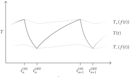
3.2. Synchronised Groups of TCLs. In the previous section we studied the stability of a uniformly distributed (continuum) population of TCLs at the 50 Hz equilibrium and found it to be stable almost everywhere in parameter space. In this section we consider the opposite extreme of possible TCL distributions, the Dirac delta distribution. That is to say, we explore the behaviour of a fully synchronised population of TCLs, all switching on and off at the same time, all with the same temperature, and (again) identical parameters. This is

T

t

T+(f(t))

T−(f(t))

t／．n t／＆＆n t／．n+1 t／＆＆n+1

T(t)

Figure 2: Illustration of the𝑛th and(𝑛 + 1)th switching events of the fully synchronised population and the frequency-sensitive temperature set points𝑇₋(𝑓(𝑡))and𝑇₊(𝑓(𝑡)).

equivalent to a single TCL with the power consumption of the whole population.

3.2.1. Mapping the Switch Times. We begin by constructing a map from one (whole population) switch on event to the next. We show that under certain conditions such a mapping is a contraction. Let the subscript𝑛denote the𝑛th switch on and𝑛th switch off event. Without loss of generality, suppose that after our initial start time𝑡₀the next switch event is the population switching on. This implies that, for all𝑛 ∈ N,

𝑡OFF

𝑛 > 𝑡ON𝑛 . Figure 2 illustrates the notation. Hence the

amount of time the population spends switched on following the𝑛th switch on event is given by

𝑡OFF

𝑛 − 𝑡ON𝑛 = _𝛼1log(

𝑇0

+− 𝛽+𝑓𝑛ON− 𝑇ON

𝑇0

−− 𝛽−𝑓𝑛OFF− 𝑇ON

) , (40a)

where𝑓_𝑛ON, 𝑓_𝑛OFFare the frequencies at the𝑛th switch on and off times. The amount of time spent switched off following the

𝑛th switch off is given by

𝑡ON

𝑛+1− 𝑡OFF𝑛 =_𝛼1log(𝑇OFF− 𝑇

0

−+ 𝛽−𝑓𝑛OFF

𝑇OFF− 𝑇+0+ 𝛽+𝑓𝑛+1ON

) . (40b)

Assuming, as for the numerical analysis in Section 3.1, that the system has no damping, we set𝛾 = 0in (12) for𝑓(𝑡)̇ . In a synchronised population, at time𝑡all TCLs are either on (𝜌(𝑡) = 1) or off (𝜌(𝑡) = 0). Then we can define constants

𝑐ON, 𝑐OFF> 0such that

̇

𝑓

={_{

{

−𝑐ON fl𝑐𝑃𝑐(𝜌∗− 1) when the population is on

+𝑐OFF fl𝑐𝑃𝑐𝜌∗when the population is off.

(41)

Hence the values of𝑓at the switch off and on times are given by the piecewise-linear functions

𝑓OFF

𝑛 = 𝑓𝑛ON− 𝑐ON(𝑡OFF𝑛 − 𝑡𝑛ON) (42a)

𝑓ON

After substituting for the switching times using (40a) and (40b) and rearranging, these become

𝑓OFF

𝑛 −𝑐ON_𝛼 log(𝑇−0− 𝛽−𝑓𝑛OFF− 𝑇ON)

= 𝑓ON

𝑛 −𝑐ON_𝛼 log(𝑇+0− 𝛽+𝑓𝑛ON− 𝑇ON)

(43a)

𝑓ON

𝑛+1+𝑐OFF_𝛼 log(𝑇OFF− 𝑇+0+ 𝛽+𝑓𝑛+1ON)

= 𝑓OFF

𝑛 +𝑐OFF_𝛼 log(𝑇OFF− 𝑇−0+ 𝛽−𝑓𝑛OFF) .

(43b)

Now since each side of (43a) and (43b) are functions of only one of the𝑓_𝑛∙variables, we can explicitly name them as such

𝜙_ON− (𝑓OFF

𝑛 )fl𝑓𝑛OFF

−𝑐ON

𝛼 log(𝑇−0− 𝛽−𝑓𝑛OFF− 𝑇ON)

(44a)

𝜙+_ON(𝑓ON

𝑛 )fl𝑓𝑛ON

−𝑐ON

𝛼 log(𝑇+0− 𝛽+𝑓𝑛ON− 𝑇ON)

(44b)

𝜙−_OFF(𝑓OFF

𝑛 )fl𝑓𝑛OFF

+𝑐OFF

𝛼 log(𝑇OFF− 𝑇−0+ 𝛽−𝑓𝑛OFF)

(44c)

𝜙_OFF+ (𝑓ON

𝑛+1)fl𝑓𝑛+1ON

+𝑐OFF

𝛼 log(𝑇OFF− 𝑇+0+ 𝛽+𝑓𝑛+1ON) .

(44d)

Each of the four 𝜙 functions is increasing and therefore invertible, and so we can write

𝑓OFF

𝑛 = 𝜙−

−1

ON𝜙+ON(𝑓 ON

𝑛 ) (45a)

𝑓ON

𝑛+1 = 𝜙+

−1

OFF𝜙−OFF(𝑓𝑛OFF) (45b)

and therefore

𝑓ON

𝑛+1= 𝜙+

−1

OFF𝜙OFF− 𝜙−

−1

ON𝜙+ON(𝑓𝑛ON) , (45c)

which is a mapping from the frequency at one switch on event to the frequency at the next. The mapping is a contraction iff

󵄨󵄨󵄨󵄨

󵄨󵄨󵄨(𝜙+OFF−1 𝜙−OFF𝜙−

−1

ON𝜙ON+ )

󸀠󵄨󵄨󵄨󵄨

󵄨󵄨󵄨 < 1 (46)

iff 󵄨󵄨󵄨󵄨󵄨󵄨󵄨󵄨

󵄨󵄨 (𝜙− OFF) 󸀠 (𝜙+ OFF) 󸀠 (𝜙+ ON) 󸀠 (𝜙− ON) 󸀠󵄨󵄨󵄨󵄨󵄨󵄨󵄨󵄨

󵄨󵄨< 1

(evaluated at the appropriate places) . (47) Note that (𝜙− OFF) 󸀠 (𝜙+ OFF) 󸀠 =

1 + 𝛽₋𝑐_OFF/ [𝛼 (𝑇_OFF− 𝑇+

𝑛)]

1 + 𝛽₊𝑐OFF/ [𝛼 (𝑇OFF− 𝑇𝑛+1+ )]

< 1

iff 𝛽+

𝛽₋ >

𝑇_OFF− 𝑇+ 𝑛+1

𝑇OFF− 𝑇𝑛− .

(48)

Similarly

(𝜙+_ON)󸀠 (𝜙−

ON)

󸀠 =

1 + 𝛽₊𝑐ON/ [𝛼 (𝑇𝑛+− 𝑇ON)] 1 + 𝛽₋𝑐_ON/ [𝛼 (𝑇−

𝑛 − 𝑇ON)]

< 1

iff 𝛽+

𝛽₋ <

𝑇_𝑛+− 𝑇ON 𝑇−

𝑛 − 𝑇ON

.

(49)

Therefore a sufficient condition for the mapping to be a contraction is that

𝛽₊ 𝛽− ∈ (

𝑇OFF− 𝑇𝑛+1+

𝑇OFF− 𝑇𝑛− ,

𝑇+

𝑛 − 𝑇ON

𝑇−

𝑛 − 𝑇ON

) (50)

which is a nonempty interval (containing {1}), so long as

𝑇_ON < 𝑇−

𝑛 < 𝑇𝑛+ < 𝑇OFF and 𝑇𝑛− < 𝑇𝑛+1+ for all 𝑛. It is

worth recalling our earlier condition on the values of𝛽_±(7) which also imposed that𝛽₊/𝛽₋ belong to an open interval containing{1}.

3.2.2. Solving for the Periodic Solution. The contraction prop-erty of the mapping𝑓_𝑛ON 󳨃→ 𝑓_𝑛+1ON (45c) under the above conditions implies that there is an attracting fixed point so long as𝑇_ON < 𝑇_𝑛− < 𝑇_𝑛+ < 𝑇_OFF, and hence a periodic solution for the synchronised population. We now seek to solve for this periodic solution. Denote by𝑙_ONand𝑙_OFFthe amount of time spent on and off during one (periodic) cycle, respectively. Since power consumption for the population is constant during each on/off phase, the frequency moves linearly between upper and lower values which we denote by

𝑓₊and𝑓₋. Therefore the temperature of the population will cycle between upper and lower set points, given by𝑇₊0− 𝛽₊𝑓₊ and𝑇₋0− 𝛽₋𝑓₋, respectively. Equations (42a) and (42b) show us that

𝑓₋= 𝑓₊− 𝑐ON𝑙ON (51a) 𝑓₊= 𝑓₋+ 𝑐OFF𝑙OFF. (51b)

The temperature evolution equations (3a) and (3b) allow us to express the switch on and switch off temperatures as follows:

𝑇₊0− 𝛽₊𝑓₊ = (𝑇₋0− 𝛽₋𝑓₋− 𝑇OFF) 𝑒−𝛼𝑙OFF+ 𝑇OFF (52a)

𝑇₋0− 𝛽₋𝑓₋ = (𝑇₊0− 𝛽₊𝑓₊− 𝑇ON) 𝑒−𝛼𝑙ON+ 𝑇ON (52b)

which after substituting for𝑓₋ using (51a) and rearranging become

𝑓₊(𝛽₋𝑒−𝛼𝑙OFF− 𝛽

+)

= (𝑇₋0− 𝑇OFF+ 𝛽−𝑐ON𝑙ON) 𝑒−𝛼𝑙OFF+ 𝑇OFF− 𝑇+0,

(53a)

𝑓₊(𝛽₊𝑒−𝛼𝑙ON− 𝛽

−)

= (𝑇₊0− 𝑇ON) 𝑒−𝛼𝑙ON+ 𝑇ON− 𝑇−0− 𝛽−𝑐ON𝑙ON.

20 40 60 80 100 120 140 0

Time (mins)

−30 −20 −10 0 10 20

T

emp

er

at

u

re

(

∘ C)

∗= 0.091

∗=0.182

∗=0.273

∗=0.364

∗=0.455

∗=0.545

∗=0.636

∗=0.727

∗=0.818

∗=0.909

Figure 3: One cycle of the single group solution for different values

of𝜌∗when𝜌₀≈ 0.3355. They include values that lead to unrealistic

results for real fridges but are there to illustrate the effect.

Now we have two equations in terms of𝑓₊, 𝑙_ON and 𝑙_OFF, which we can combine into one equation and eliminate𝑓₊,

(𝛽₊𝑒−𝛼𝑙ON− 𝛽

−)

⋅ [(𝑇₋0− 𝑇OFF+ 𝛽−𝑐ON𝑙ON) 𝑒−𝛼𝑙OFF+ 𝑇OFF− 𝑇+0]

= (𝛽−𝑒−𝛼𝑙OFF− 𝛽+)

⋅ [(𝑇₊0− 𝑇_ON) 𝑒−𝛼𝑙ON+ 𝑇

ON− 𝑇−0− 𝛽−𝑐ON𝑙ON] . (54)

We can also express𝑙_OFFin terms of𝑙_ONby summing (51a) and (51b) to give

𝑐ON𝑙ON= 𝑐OFF𝑙OFF or, equivalently, (1 − 𝜌∗) 𝑙ON− 𝜌∗𝑙OFF= 0

(55)

and so (53b) and (55) form a pair of coupled equations for𝑙_ON and𝑙_OFF, which can be solved numerically. Figure 3 shows one temperature cycle for the single group under different choices for𝜌∗. Denote by𝜌₀the value of𝜌when𝑓 = 0. As

𝜌∗gets further away from𝜌₀the solutions drift further from the uncoupled temperature range (2–7∘C). The cycle lengths are symmetric about𝜌∗ = 1/2but the TCLs consume more power per cycle as𝜌∗increases.

To begin some analysis of the stability of this fully synchronised solution we address the question: given a pop-ulation split into two synchronised groups, will the groups merge into one fully synchronised population, or will they remain distinct forever?

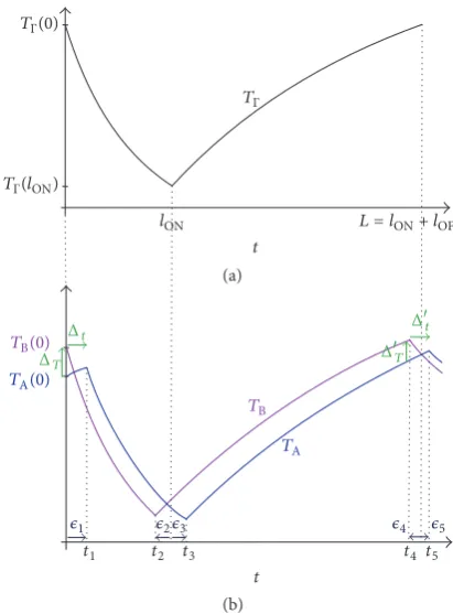
3.2.3. Two-Group Dynamics. Suppose we have a population of frequency-sensitive TCLs that are split into two synchro-nised groups. We would like to understand the dynamics of the switch times, and we ask whether, given sufficient time, the groups will merge, or whether they will remain distinct, possibly settling down to separated periodic solutions. In

TΓ(0)

TΓ(l／．)

TΓ

l／． L = l／．+ l／＆＆

t

TA TB TB(0)

TA(0) ΔT

Δt

Δ T

Δt

t1 t2 t3 t4 t5

t

(a)

(b)

1 23 4 5

Figure 4: Linearisation about the single group solution. (a) Single group solution𝑇_Γ(𝑡). (b) Temperature cycling of groups A and B close to the single group solution.

particular, we consider the initial difference between the switch on times Δ_𝑡 to be very small and the switch on temperatures very close to the single group periodic solution from the previous subsection.

Let Γdenote the single group periodic solution, which cycles periodically through temperature space with temper-ature𝑇_Γ(𝑡). As before, we denote the switched on duration in this solution by𝑙_ONand the switched off duration by𝑙_OFF. Suppose that the population is split into two groups A and B, such that proportion𝜎belongs to group A, and proportion

1 − 𝜎belongs to group B. Suppose also that group B switches on at time𝑡 = 0, followed soon after by group A switching on, at time𝑡₁> 0. Then after a time period of length similar to𝑙_ON group B switches off, which is again followed shortly after by group A switching off. After a time period similar to𝑙_OFFeach of the groups then switches back on. We shall assume that the switching order does not change, since if they do swap, we need only repeat this process with𝜎 replaced by1 − 𝜎. Simulations show that the switching order will not continue to change indefinitely.

We would like to compare the temperature cycles of these two groups with the single group periodic solutionΓ. Without loss of generality suppose that group B initially switches on at the same time as a fully synchronised population solution. We compare the cycling of the groups A and B using the following measures, along with all those shown in Figure 4. LetΔ_𝑇 fl



0.2 0.4 0.6 0.8 1.0

0.0



0.5 1.0 1.5 2.0

(a) Full interval



0.96 0.98 1.00 1.02 1.04

0.35 0.40 0.45 0.50 0.55 0.60 0.65 0.70

0.30



(b) Enlargement

Figure 5: Solutions for𝜆(see (61)) (solid lines) for different values of𝜌∗. Dashed lines show reflection in𝜎 = 1/2to show the effect of reversing the switching order of the groups. Blue:𝜌∗ = 0.1, yellow:𝜌∗ = 0.2, green:𝜌∗ = 0.3, and red:𝜌∗ = 0.4. Black line shows the boundary of stability (stable below, unstable above). The results are identical when𝜌∗is replaced by1 − 𝜌∗. (b) shows an enlargement centred

at𝜎 = 1/2, showing that either switching order of the groups leads to𝜆₂> 1on a small interval of𝜎. In this case the groups never merge and

in all other cases they will.

Δ󸀠_𝑡 fl 𝑡5− 𝑡4, the time difference between the two groups

switching on the first and second times, respectively. Further notation is shown in Figure 4.

In order to calculate Δ󸀠_𝑇 and Δ󸀠_𝑡 we need to calculate the switch times and temperatures of the two groups at each switch event leading up to𝑡₅. Solving for the switch times and temperatures when there are two groups is a little more complicated than for the fully synchronised case. It requires solving the temperature set point equations using the system conditions at the previous switch and the equation for 𝑓̇ which now takes one of four values depending on which combination of groups is switched on (both, neither, A only, or B only). We begin by making the simplifying assumption

𝛽₋ = 𝛽₊ fl 𝛽. Now since group A is switching on at time𝑡₁ and group B switched off at time 0,

𝑇A(𝑡1) = 𝑇+0− 𝛽𝑓 (𝑡1)

𝑓 (𝑡₁) = 𝑓 (0) − 𝑐𝑃𝑐(1 − 𝜎 − 𝜌∗) 𝑡1

𝑓 (0) =_𝛽1(𝑡0₊− 𝑇B(0))

∴ 𝑇_A(𝑡1) = 𝑇B(0) + 𝛽𝑐𝑃𝑐(1 − 𝜎 − 𝜌∗) 𝑡1.

(56a)

In addition, by the temperature evolution equations,

𝑇A(𝑡1) = (𝑇A(0) − 𝑇OFF) 𝑒−𝛼𝑡1+ 𝑇OFF. (56b)

Equating (56a) and (56b) and introducing our new notation give

𝛽𝑐𝑃_𝑐(1 − 𝜎 − 𝜌∗) Δ_𝑡+ Δ_𝑇

= (𝑇A(0) − 𝑇OFF) (𝑒−𝛼Δ𝑡− 1) .

(57)

If we write𝑇_A(0) = 𝑇_Γ(0) + 𝛿𝑇_A(0)and take𝛿𝑇_A(0)andΔ_𝑡 small, then

Δ𝑇= (𝑇Γ(0) + 𝛿𝑇A(0) − 𝑇OFF) (𝑒−𝛼Δ𝑡− 1)

− 𝛽𝑐𝑃_𝑐(1 − 𝜎 − 𝜌∗) Δ_𝑡 (58)

and linearising inΔ_𝑡gives

Δ𝑇≈ 𝜉Δ𝑡, (59)

where

𝜉fl𝛼 (𝑇OFF− 𝑇Γ(0)) − 𝛽𝑐𝑃𝑐(1 − 𝜎 − 𝜌∗) . (60)

More generally, at each switch event we have the temperature evolution equations that describe the temperature of each group as a function of their temperature at the previous switch (such as (56b)) and an additional equation for the temperature of the switching group, using the temperature set point equations (such as (56a)). WritingΔ󸀠_𝑇= 𝑇_B(𝑡₄)−𝑇_A(𝑡₄) and linearising about the single group solution, we find in Appendix B thatΔ󸀠_𝑇= 𝜆Δ_𝑇where

𝜆fl(1 − 𝛼 (𝑇OFF− 𝑇ON)

𝛼 (𝑇OFF− 𝑇Γ(0)) − 𝛽𝑐𝑃𝑐(1 − 𝜎 − 𝜌∗))

⋅ (1 − 𝛼 (𝑇OFF− 𝑇ON)

𝛼 (𝑇Γ(𝑙ON) − 𝑇ON) + 𝛽𝑐𝑃𝑐(𝜎 − 𝜌∗) )

⋅ 𝑒−𝛼𝐿.

(61)

So[−1, +1]is a left eigenvector of the linearised map in the space of(𝛿𝑇A

𝛿𝑇B)with eigenvalue𝜆. We can plot𝜆 against𝜎

∗

(1 − , ∗)= 1 (, ∗_{)= 1}

Attracting if Attracting if

A switches first B switches first

Repelling in both cases

0.0 0.2 0.4



0.6 0.8 1.0

0.0 0.2 0.4 0.6 0.8 1.0

Figure 6: Bifurcation diagram for the stability of the single group solution to splitting in two. Stable if the parameters lie in the yellow or blue regions (the groups will ultimately merge); unstable in the green parameter region (the groups will never merge). Boundary lines are solutions to (61) as a function of𝜎(or1 − 𝜎to capture switching order reversal) and𝜌∗.

our parameter values (taken from Table 2 with the exception of𝛽 = 0.1which has been reduced to limit the rate of change of the frequency and ensure model validity), see Appendix C for details, and therefore the stability is governed by𝜆.

By solving for the dividing case 𝜆 = 1 we can create a bifurcation diagram in terms of the parameters 𝜎 and

𝜌∗ _{to show where the single group solution is attracting}

and repelling. Figure 6 sketches the solution, along with the solution for the case when the switching order of the groups is reversed, found by replacing𝜎 with 1 − 𝜎. If in either case (group A switching first or group B switching first) the solution is attracting, then the two groups will merge together into the one group solution. However, if both cases have unstable dynamics then the solutions will never merge. Simulations show that in this parameter region the two groups will settle down to a fixed phase distance apart. If the solution is attracting for one switching order and repelling for the other, we find that the typical behaviour is for a small separation in the unstable direction to grow until the phase difference becomes almost a whole cycle, when they merge. Figure 7 illustrates how the cycles of the two groups can change over time relative to one another, depending on which of the three regions in the bifurcation diagram their parameters belong to.

What these results show is that when a population is split into two groups, if they are sufficiently similar in size then they will remain apart, effectively trying to counteract one another and balance the frequency fluctuations. Conversely, if one of the groups is significantly larger (“significantly” here depends on the size of𝜌∗, and may be very small if𝜌∗ ≈

0.5) than the other then it will have too strong an effect on

the frequency and “pull” on the smaller group’s cycle. The closer the proportion switched on in equilibrium is to the proportion switched off (i.e., the closer it is to 0.5), the more similar the groups have to be in size to remain distinct.

With more than two groups of TCLs the modelling becomes far more complicated, since there are now far more possibilities to be considered for the switching order of the groups. Simulations have shown that for three groups it is possible for all three cycles to settle down to a fixed, separated pattern. This occurs if the groups are very similar in size, just as in the two-group case. Once one group is too large (or too small), the groups collapse into two, before synchronising completely. Taking the number of groups to infinity is equiva-lent to modelling a continuum of TCLs as in Section 3.1. Tak-ing all groups of equal size and uniformly distributed in phase

𝜃 is equivalent to the continuum population equilibrium studied earlier. From above we found analytically that small perturbations to the population distribution should relax back to the uniform distribution, that is, that the equilibrium was stable. Now we find that if the population is discretised into 2 (and hypothetically𝑁) groups then so long as they are of close to equal sizes, they will attempt to settle the frequency back to its nominal value by “spreading out” their cycles.

In reality we will never have a continuum of TCLs, and they may exhibit nonlinear dynamics not captured by our analysis. This motivates our use of simulations to gain further insights into how a large population of TCLs would behave according to our switching rules and how the grid frequency would be affected.

4. Simulations

4.1. Perturbations of a Uniform Distribution of TCLs. In Section 3.1 we analysed the stability of a large population of TCLs uniformly distributed in each part of the on/off cycle. In this section we simulate a large population of fridges with initial conditions close to the equilibrium distribution (the uniform distribution) and compare the results with our analytical work.

Group A temperature cycling Group B temperature cycling

(a)(, ∗) < 1, blue parameter region in Figure 6

(b)(1 − , ∗) < 1, yellow parameter region in Figure 6

(c)(, ∗) > 1, (1 − , ∗) > 1, green parameter region in Figure 6

Figure 7: Illustration of the three types of cycling behaviour of two groups relative to one another, based on simulations. Arrows indicate the occurrence of many cycles and the central illustrations are snapshots of the cycling behaviour between the start and the final behaviour. Synchronisation occurs in cases (a) and (b), while in case (c) each group tends towards a fixed phase difference apart.

Table 3: Parameter values for plots in Figures 8, 9, and 10.

Plot number 𝜌_on(0) Δ𝑢

a(i) 𝜌∗ 0

a(ii) 𝜌∗ 0.1

a(iii) 𝜌∗ 0.25

a(iv) 𝜌∗ 0.5

b(i) 1.5𝜌∗ 0

b(ii) 1.5𝜌∗ 0.1

b(iii) 1.5𝜌∗ 0.25

b(iv) 1.5𝜌∗ 0.5

To perturb the TCL distribution𝑢(𝜃) we can alter the number of TCLs switched on or off from the equilibrium proportions𝜌∗and(1 − 𝜌∗), respectively, and we can perturb the uniform distributions within each on/off half of the

𝜃 interval. We choose to perturb the distributions by the addition of a sine wave to𝑢∗, and we refer to the normalised wave peak amplitudeΔ𝑢(normalised by dividing by𝑢∗). This normalisation means that when we plot𝑢(𝜃, 0)/𝑢∗, the zero perturbation case is 1 for all𝜃both on and off and the results are more clear. Table 3 shows eight combinations of choices for these perturbation parameters. All other parameters are as stated in Table 2.

Figure 8 shows the effects of these perturbations on the initial conditions in each case, plotting 𝑢(𝜃, 0)/𝑢∗ against

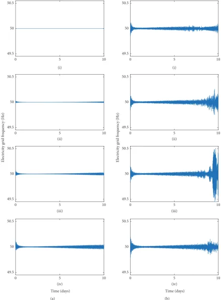
𝜃. Figure 9 shows the final fridge distributions after ten days. The unperturbed case a(i) has remained uniform, while the peaks of the perturbation cases have all grown by varying amounts. In cases a(ii)–a(iv) (no perturbation to the proportion switched on) the final distributions exhibit increasing levels of synchronisation, but the clustering is far less than in cases b(i)–b(iv) which see the population synchronised into seven or fewer groups. The effects of this synchronisation on the electricity grid frequency can be seen in Figure 10.

Interestingly, in each case with perturbations, the fre-quency oscillations initially die down to close to 50 Hz. This means that to begin with the fridges are controlling the frequency oscillations caused by their initial condition per-turbations. This aligns with our analysis from Section 3.1, in which we found that the uniform distribution of a continuum population is stable to small perturbations. What that analysis was unable to capture was the long-term effects of frequency sensitivity. In each case the frequency oscillations grow after less than a day, becoming very large in several cases. Before the large spikes in b(iii) we see that the frequency oscillations shrink down. This shows the inherently volatile nature of the system and potentially explains why the oscillations in b(iv) are ultimately less severe. It could be that these lower oscillations will shortly become much larger. In either case, the size of most of the final oscillations would be too large for the system to cope without frequency response from other providers.

These simulations reveal that while a homogeneous popu-lation of TCLs will act to dampen system perturbations, their behaviour to support the electricity grid will, given sufficient time, lead to further oscillations. The larger the perturbations are, the sooner these detrimental effects will occur.

(i)

(ii)

(iii)

(iv)

S

caled T

CL distr

ib

u

tio

n

u/u

∗

0 0.5 1 1.5 2 2.5 0 0.5 1 1.5 2 2.5 0 0.5 1 1.5 2 2.5 0 0.5 1 1.5 2 2.5

0 0.5 1

−0.5 −1



0 0.5 1

−0.5 −1

0 0.5 1

−0.5 −1

0 0.5 1

−0.5 −1

(ii) (i)

(iii)

(iv)

S

caled T

CL distr

ib

u

tio

n

u/u

∗

0 0.5 1 1.5 2 2.5

0 0.5 1 1.5 2 2.5

0 0.5 1 1.5 2 2.5

0 0.5 1 1.5 2 2.5

0 0.5 1

−0.5 −1



0 0.5 1

−0.5 −1

0 0.5 1

−0.5 −1

0 0.5 1

−0.5 −1

(a) (b)

(a) (b) (i)

(ii)

(iii)

(iv)

S

caled T

CL distr

ib

u

tio

n

u/u

∗

0 20 40 0 20 40 0 20 40 0 20 40

−0.5 0 0.5 1

−1



−0.5 0 0.5 1

−1

−0.5 0 0.5 1

−1

−0.5 0 0.5 1

−1

S

caled T

CL distr

ib

u

tio

n

u/u

∗

(i)

(ii)

(iii)

(iv) 0

20 40 0 20 40

0 20 40

0 20 40

−0.5 0 0.5 1

−1



−0.5 0 0.5 1

−1

−0.5 0 0.5 1

−1

−0.5 0 0.5 1

−1

(a) (b) (i)

(ii)

(iii)

Time (days)

5 10

0

(iv)

5 10

0

5 10

0

5 10

0

49.5 50 50.5 49.5 50 50.5 49.5 50 50.5 49.5 50 50.5

E

lec

tr

ici

ty gr

id f

req

uenc

y (H

z)

(i)

(ii)

(iii)

(iv)

5 10

0

Time (days)

5 10

0

5 10

0

5 10

0

49.5 50 50.5 49.5 50 50.5 49.5 50 50.5 49.5 50 50.5

E

lec

tr

ici

ty gr

id f

req

uenc

y (H

z)

Demand

Kinetic energy

Historic frequency

Calculate underlying imbalance

Response holdings

Underlying imbalance

Fridge conditions

Calculate frequency response delivery

Calculate new fridge conditions

Calculate new frequency

Response from other providers Fridge states and

temperatures

Inp

u

ts

It

era

ti

ve

lo

o

p

Ou

tp

u

ts

Calculate demand at

Demand at

50 （Ｔ 50 （Ｔ

Figure 11: Simulation methodology diagram. Rhombi indicate input or calculated data/simulated data, and rectangles indicate meth-ods/calculations. Events occur from top to bottom with the exception of the dashed arrows which form the iterative loop.

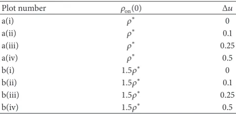
period, and the reduction in the amount of response that other providers needed to supply because of the contribution from the fridges.

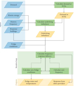
4.2.1. Methods. We simulate a population of TCLs (specifi-cally fridges) that respond to the grid frequency according to the rules in Section 2.1. We use various historic data from National Grid to model real system conditions and simulate the effects of a frequency-sensitive fridge population acting on the GB system. By considering the population in the context of real data including response provision from other sources such as power generators, we are able to get a better understanding of the potential impact of the fridges compared to, say, modelling them in isolation responding to a one-off frequency event.

Figure 11 gives an overview of the simulation process. Rhombi indicate inputs and outputs; rectangles indicate methods used in the simulation. Methods are applied work-ing downwards, except for the dashed arrows which create an iterative loop.

4.2.2. Inputs. As shown in Figure 11, there are four types of data input, in addition to the fridge population initial

conditions. We use 36 consecutive ten-day data samples from the period July 2015–June 2016.

Kinetic energy data is an estimate for the total kinetic energy in MVAs (megavolt-ampere seconds) [55]. Values are calculated by summing the kinetic energy of all run-ning synchronised generators (a generator-specific constant provided to the System Operator by each power generator) with an estimate of kinetic energy from demand. The kinetic energy data provided (confidentially from National Grid) is per settlement period (settlement periods split the day into 48 half hour units starting on the hour and half hour) and repeats each value for the full 30 minutes (rather than interpolating). Typical kinetic energy values are in the range 20000–40000 MVAs.

Demand data consists of per-second metered demand from National Grid. This is a sum of the power leaving the electricity transmission system, including any power exports through the interconnectors. Half-hourly demand data is accessible via National Grid’s “Data Explorer” [56].

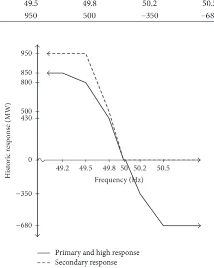
Table 4: Illustrative historic response holding data behind Figure 12.

Primary Secondary High

Frequency trigger (Hz) 49.2 49.5 49.8 49.5 49.8 50.2 50.5

Response (MW) 850 800 430 950 500 −350 −680

National Grid has undergone a cleaning process that takes advantage of the multiple readings. It is available via National Grid’s “Enhanced Frequency Response” [57].

Response holdingsare the amount of frequency response delivery in MW (as a function of grid frequency) that National Grid expects each second. Response holdings are positive (or negative) for “low (high) frequency response delivery” when the frequency is below (above) 50 Hz, respec-tively. For each time step (1 second), 9 different values for response holding are listed. These take the form of primary, secondary, and high response.

Primary response values are given for trigger points at 49.9 Hz, 49.5 Hz, and 49.2 Hz. This means that at these fre-quencies the power response provided through various types of primary response service are the historic response holding values given, subject to a 1 second reaction delay. We assume that the response increases linearly from 0 between 49.985 Hz and 49.8 Hz and likewise linearly between all other frequency trigger values. Below 49.2 Hz the response is assumed to be the constant 49.2 Hz response value. The starting frequency trigger value of 49.985 Hz is used to take into account the Grid Code deadband of (50 ± 0.015) Hz, within which response is not required. Secondary response values are given for frequency trigger points 49.8 Hz and 49.5 Hz, and response is modelled in the same was as for primary response, only with an 11 s response delay. High response values have trigger points 50.2 Hz and 50.5 Hz. Just as for primary response, the time lag is 1 s and again, response is modelled as linear interpolation through these points, starting at the edge of the deadband at 50.015 Hz and remaining constant beyond 50.5 Hz. Figure 12 illustrates an example of how response holding data (Table 4) are interpreted in the model. Values given are indicative only of possible values.

Fridge conditions are the initial on/off state and initial temperature of each fridge in the population. For the simu-lations presented here we take the zero perturbation case a(i) in Table 3 from the previous section.

4.2.3. Calculating the Demand at 50 Hz. Deviations in grid frequency away from 50 Hz affect the total system demand. We make the assumption that demand increases linearly by approximately 2.5% of its value at 50 Hz for every 1 Hz increase in frequency above 50 Hz (and decreases by the same amount as frequency decreases below 50 Hz). In order to know the demand at the nominal frequency, “demand at 50 Hz,” Dem_𝜔0(𝑡), we need to calculate it from the (mea-sured) demand data input,𝐷(𝑡).

𝐷 (𝑡) =Dem_𝜔0(𝑡) [1 + 0.025 (𝑓 (𝑡) − 50)] (62)

Dem_𝜔0(𝑡) = 𝐷 (𝑡)

1 + 0.025 (𝑓 (𝑡) − 50). (63)

Primary and high response Secondary response

−680 −350

0 430 500 800 850 950

H

ist

o

ric r

esp

o

n

se

(MW)

49.5 49.8 50 50.2 50.5 49.2

Frequency (Hz)

Figure 12: Representative historic response data with interpolation method for primary response (solid line below 50 Hz), secondary response (dashed line), and high response (solid line above 50 Hz). Zero response in the deadband (50 ± 0.015)Hz.

4.2.4. Calculating the Underlying Imbalance. In order to calculate the effects of the fridge population on the system frequency, we first need to calculate the underlying supply-demand imbalance (in MW) that caused the original system frequency deviations away from 50 Hz. At this point it is necessary to distinguish between two important, similar-sounding terms:underlying imbalanceandtotal imbalance. By underlying imbalance, Imb_under(𝑡), we mean the generation-demand imbalance that occurs independently of the system frequency. This may be due to, for example, fluctuations in wind or solar power generation or discrepancies between the total predicted system demand and the actual real-time demand. In contrast, total imbalance, Imb_tot(𝑓, 𝑡), includes both the underlying imbalance and, additionally, what we shall refer to asdynamic imbalance.