Learning Explicit and Implicit Structures for Targeted Sentiment Analysis

Proceedings of the 2019 Conference on Empirical Methods in Natural Language Processing 5478

Learning Explicit and Implicit Structures for Targeted Sentiment Analysis

Hao Li and Wei Lu

StatNLP Research Group

Singapore University of Technology and Design hao [email protected]

[email protected]

Abstract

Targeted sentiment analysis is the task of jointly predicting target entities and their as-sociated sentiment information. Existing re-search efforts mostly regard this joint task as a sequence labeling problem, building models that can capture explicit structures in the out-put space. However, the importance of cap-turing implicit global structural information that resides in the input space is largely unex-plored. In this work, we argue that both types of information (implicit and explicit structural information) are crucial for building a success-ful targeted sentiment analysis model. Our experimental results show that properly cap-turing both information is able to lead to bet-ter performance than competitive existing ap-proaches. We also conduct extensive experi-ments to investigate our model’s effectiveness and robustness1_.

1 Introduction

Targeted sentiment analysis (TSA) is an impor-tant task useful for public opinion mining (Pang and Lee, 2008; Liu, 2010; Ortigosa et al., 2014;

Smailovi´c et al.,2013;Li and Wu,2010). The task focuses on predicting the sentiment information towards a specific target phrase, which is usually a named entity, in a given input sentence. Currently, TSA in the literature may refer to either of the two possible tasks under two different setups: 1) pre-dicting the sentiment polarity for a given specific target phrase (Dong et al.,2014;Wang et al.,2016;

Zhang et al.,2016;Xue and Li,2018); 2) jointly predicting the targets together with the sentiment polarity assigned to each target (Mitchell et al.,

2013; Zhang et al., 2015; Li and Lu, 2017; Ma et al.,2018). In this paper, we focus on the latter setup which was originally proposed byMitchell

1_{We release our code at http://www.statnlp.}

org/research/st.

+ + 00

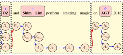
OZ and Shim Lim perform amazing magic on AGT 2018

Figure 1: TSA with targets in bold and their associated sentiment on top. Boundaries for the sentiment scope are highlighted in dashed boxes.

et al. (2013). Figure 1 presents an example sen-tence containing three targets. Each target is asso-ciated with a sentiment, where we use+ for de-noting positive polarity, 0 for neutral and − for negative.

Existing research efforts mostly regard this task as a sequence labeling problem by assign-ing a tag to each word token, where the tags are typically designed in a way that capture both the target boundary as well as the targeted sentiment polarity information together. Exist-ing approaches (Mitchell et al., 2013; Zhang et al., 2015;Ma et al.,2018) build models based on conditional random fields (CRF) (Lafferty et al.,2001) or structural support vector machines (SSVM) (Taskar et al.,2005;Tsochantaridis et al.,

2005) to explicitly model the sentiment infor-mation with structured outputs, where each tar-geted sentiment prediction corresponds to exactly one fixed output. While effective, such mod-els suffer from their inability in capturing cer-tain long-distance dependencies between senti-ment keywords and their targets. To remedy this issue,Li and Lu(2017) proposed their “sentiment scope” model to learn flexible output representa-tions. For example, three text spans with their corresponding targets in bold are presented in Fig-ure1, where each target’s sentiment is character-ized by the words appearing in the corresponding text span. They learn from data for each target a latent text span used for attributing its sentiment, resulting inflexibleoutput structures.

limi-tations with the approach of Li and Lu (2017). First, their model requires a large number of hand-crafted discrete features. Second, the model relies on a strong assumption that the latent sentiment spans do not overlap with one another. For exam-ple, in Figure1, their model will not be able to cap-ture the interaction between the target word “OZ” in the first sentiment span and the keyword “amaz-ing” due to the assumptions made on the explicit structures in the output space. One idea to resolve this issue is to design an alternative mechanism to capture such useful structural information that re-sides in the input space.

On the other hand, recent literature shows that feature learning mechanisms such as self-attention have been successful for the task of sentiment prediction when targets are given (Wang and Lu,

2018;He et al., 2018;Fan et al.,2018) (i.e., un-der the first setup mentioned above). Such ap-proaches essentially attempt to learn richimplicit structural information in the input space that cap-tures the interactions between a given target and all other word tokens within the sentence. Such implicit structures are then used to generate sen-timent summary representation towards the given target, leading to the performance boost.

However, to date capturing rich implicit struc-tures in the joint prediction task that we focus on (i.e., the second setup) remains largely unex-plored. Unlike the first setup, in our setup the targets are not given, we need to handle exponen-tially many possible combinations of targets in the joint task. This makes the design of an algorithm for capturing both implicit structural information from the input space and the explicit structural in-formation from the output space challenging.

Motivated by the limitations and challenges, we present a novel approach that is able to efficiently and effectively capture the explicit and implicit structural information for TSA. We make the fol-lowing key contributions in this work:

• We propose a model that is able to prop-erly integrate bothexplicitandimplicit struc-tural information, called EI. The model is able to learn flexible explicit structural in-formation in the output space while being able to efficiently learn rich implicit struc-tures by LSTM and self-attention for expo-nentially many possible combinations of tar-gets in a given sentence.

• We conducted extensive experiments to

vali-+ + 0

OZ and Shim Lim perform amazing magic on AGT 2018

B+ B+ B+ B0 B0

A+ A+ A+ A+ A+ A0 A0

ES,+ EB,+ EE,+ ES,0

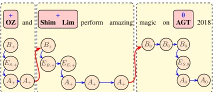
Figure 2: The structured output for representing enti-ties and their sentiments with boundaries.

date our claim that both explicit and implicit structures are indispensable in such a task, and demonstrate the effectiveness and robust-ness of our model.

2 Approach

Our objective is to design a model to extract tar-gets as well as their associated targeted sentiments for a given sentence in a joint manner. As we men-tioned before, we believe that both explicit and im-plicit structures are crucial for building a success-ful model for TSA. Specifically, we first present an approach to learn flexible explicit structures based on latent CRF, and next present an approach to ef-ficiently learn the rich implicit structures for expo-nentially many possible combinations of targets.

2.1 Explicit Structure

Motivated byLi and Lu(2017), we design an ap-proach based on latent CRF to model flexible sen-timent spans to capture better explicit structures in the output space. To do so, we firstly integrate tar-get and tartar-geted sentiment information into a label sequence by using 3 types of tags in ourEImodel:

Bp,Ap, andE,p, wherep∈ {+,−,0}indicates the sentiment polarity and∈ {B,M,E,S}denotes theBMEStagging scheme2. We explain the mean-ing of each type of tags as follows.

• Bp is used to denote that the current word is part of a sentiment span with polarityp, but appears before the target word or exactly as the first word of the target.

• Ap is used to denote that the current word is part of a sentiment span with polarityp, but appears after the target word or exactly as the last word of the target.

2

+ + 0

OZ and Shim Lim perform amazing magic on AGT 2018

B+ B+ B0 B0 B0

A+ A+ A+ A+ A+ A0 A0

ES,+ EB,+ EE,+ ES,0

Figure 3: An alternative structured output for the same example with different sentiment boundaries.

• E,pis used to denote the current word is part of a sentiment span with polarity p, and is also a part of the target. TheBMESsub-tag

denotes the position information within the target phrase. For example,EB,+represents that the current word appears as the first word of a target with the positive polarity.

We illustrate how to construct the label se-quence for a specific combination of sentiment spans of the given example sentence in Figure2, where three non-overlapping sentiment spans in yellow are presented. Each such sentiment span encodes the sentiment polarity in blue for a target in bold in pink square. At each position, we al-low multiple tags in a sequence to appear such that the edgeApBp0 in red consistently indicates the boundary between two adjacent sentiment spans.

The first sentiment span with positive (+) polar-ity contains only one word which is also the target. Such a single word target is also the beginning and the end of the target. We use three tagsB+,ES,+ andA+to encode such information above.

The second sentiment span with positive (+) polarity contains a two-word target “Shin Lim”. The word “and” appearing before such target takes a tag B+. The words “perform amazing magic” appearing after such target take a tagA+ at each position. As for the target, the word “Shin” at the beginning of the target takes tagsB+ andEB,+, while the word “Lim” at the end of the target takes tagsEE,+andA+.

The third sentiment span with neutral (0) polar-ity contains a single-word target “AGT”. Similarly, we use three tags B0, ES,0 andA0 to represent such single word target. The word “on” appear-ing before such target takes a tagB0. The word “2018” appearing afterwards takes a tagA0.

Note that if there exists a target with length larger than 2, the tagEM,pwill be used. For ex-ample in Figure2, if the target phrase “Shin Lim”

is replaced by “Shin Bob Lim”, we will keep the tags at “Shin” and “Lim” unchanged. We assign a tagEM,+at the word “Bob” to indicate that “Bob” appears in the middle of the target by following the BMEStagging scheme.

Finally, we represent the label sequence by con-necting adjacent tags sequentially with edges. No-tice that for a given input sentence and the out-put targets as well as the associated targeted senti-ment, there exist exponentially many possible la-bel sequences, each specifying a different possible combinations of sentiment spans. Figure3shows a label sequence for an alternative combination of the sentiment spans. Those label sequences repre-senting the same input and output construct a la-tent variable in our model, capturing the flexible explicit structures in the output space.

We use a log-linear formulation to parameterize our model. Specifically, the probability of predict-ing a possible outputy, which is a list of targets and their associated sentiment information, given an input sentencex, is defined as:

p(y|x) = P

hexp (s(x,y,h))

P

y0_,h0exp(s(x,y 0

,h0)) (1)

wheres(x,y,h) is a score function defined over the sentencexand the output structurey, together with the latent variable h that provides all the possible combinations of sentiment spans for the (x,y)tuple. We define E(x,y,h) as a set of all the edges appearing in all the label sequences for such combinations of sentiment spans. To com-putes(x,y,h), we sum up the scores of each edge inE(x,y,h):

s(x,y,h) = X e∈E(x,y,h)

φx(e)

where φx(e) is a score function defined over an

edgeefor the inputx.

The overall model is analogous to that of a neural CRF (Peng et al., 2009; Do et al., 2010); hence the inference and decoding follow standard marginal and MAP inference procedures. For ex-ample, the prediction ofyfollows the Viterbi-like MAP inference procedure.

2.2 Implicit Structure

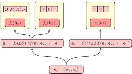
efrom our neural architecture. The three yellow boxes in Figure4compute scores for rich implicit structures from the neural architecture consisting of LSTM and self-attention.

Given an input token sequence x =

{x1, x2,· · ·, xn} of length n, we first com-pute the concatenated embeddingek = [wk;ck] based on word embedding wk and character embeddingckat positionk.

As illustrated on the left part in Figure 4, we then use a Bi-directional LSTM to encode context features and obtain hidden states hk = BiLSTM(e1,e2,· · ·,en). We use two different

linear layersft andfs to compute scores for tar-get and sentiment respectively. The linear layer

ftreturns a vector of length4, with each value in the vector indicating the score of the correspond-ing tag under theBMEStagging scheme. The lin-ear layerfsreturns a vector of length3, with each value representing the score of a certain polarity of+,0,−. We assign such scores to each type of edge as follows:

φx(Ek,pEk0+1_,p) =ft(hk)

φx(Ek,pApk) =ft(hk)

φx(BkpBpk+1) =fs(hk)p

φx(AkpApk+1) =fs(hk)p

φx(AkpBpk+10 ) =fs(hk)p

Note that the subscript p and at the right hand side of above equations denote the corresponding index of the vector thatftorfsreturns. We apply

ft on edges Ek,pEk0+1_,p and Ek_,pAk_p, since words at these edges are parts of the target phrase in a sentiment span. Similarly, we applyfs on edges

Bk

pBkp+1,AkpApk+1 and AkpBkp+10 , since words at these edges contribute the sentiment information for the target in the sentiment span.

As illustrated in Figure 4, we calculateak, the output of self-attention at positionk:

ak= n X

j=1

αk,jej

αk,j= softmax j (βk,j)

βk,j =UTReLu(W[ek;ej] +b)

whereαk,jis the normalized weight score forβk,j, and βk,j is the weight score calculated by target

ek= [wk;ck]

hk=BiLST M(e1,e2,· · ·,en) ak=Self AT T(e1,e2,· · ·,en)

ft(hk) fs(hk) gs(ak)

0

+ −

B M E S + 0 −

Figure 4: Neural Architecture

representation at positionk and contextual repre-sentation at positionj. In addition, W and b as well as the attention matrixU are the weights to be learned. Such a vectorak encodes the implicit structures between the wordxk and each word in the remaining sentence.

Motivated by the character embeddings ( Lam-ple et al.,2016) which are generated based on hid-den states at two ends of a subsequence, we en-code such implicit structures for a target similarly. For any target starting at the positionk1 and end-ing at the position k2, we could use ak1 and ak2

at two ends to represent the implicit structures of such a target. We encode such information on the edges Bk1

p Ek,p1 andEk,p2Akp2 which appear at the beginning and the end of a target phrase respec-tively with sentiment polarityp. To do so, we as-sign the scores calculated from the self-attention to such two edges:

φx(Bkp1E,pk1) =gs(ak1)p

φx(Ek,p2Apk2) +=gs(ak2)p

wheregs returns a vector of length3with scores of three polarities.

Note thathk andak could be pre-computed at every positionkand assigned to the corresponding edges. Such an approach allows us to maintain the inference time complexityO(T n), whereT is the maximum number of tags at each position which is9in this work andnis the number of words in the input sentence. This approach enablesEIto ef-ficiently learn rich implicit structures from LSTM and self-attention for exponentially many combi-nations of targets.

3 Experimental Setup

Data

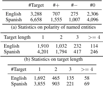
#Target #+ #− #0

English 3,288 707 275 2,306

Spanish 6,658 1,555 1,007 4,096

(a) Statistics on polarity of named entities

Target length 1 2 3 >= 4

English 1,910 1,032 232 114

Spanish 4,201 1,794 417 246

(b) Statistics on target length

#Target 1 2 3 >= 4

English 1,692 465 135 58

Spanish 3,855 903 221 69

(c) Statistics on number of targets per sentence

Table 1: Corpus Statistics of Main Dataset

contain 2,350 English tweets and 7,105 Spanish tweets, with target and targeted sentiment anno-tated. See Table1for corpus statistics.

Evaluation Metrics

Following the previous works, we report the pre-cision (P.), recall (R.) and F1 scores for target recognition and targeted sentiment. Note that a correct target prediction requires the boundary of the target to be correct, and a correct targeted sen-timent prediction requires both target boundary and sentiment polarity to be correct.

Hyperparameters

We adopt pretrained embeddings from Penning-ton et al.(2014) andCieliebak et al.(2017) for En-glish data and Spanish data respectively. We use a 2-layer LSTM (for both directions) with a hidden dimension of 500 and 6003 for English data and Spanish data respectively. The dimension of the attention weightUis 300. As for optimization, we use the Adam (Kingma and Ba,2014) optimizer to optimize the model with batch size 1 and dropout rate0.5. All the neural weights are initialized by Xavier (Glorot and Bengio,2010).

Training and Implementation

We train our model for a maximal of 6 epochs. We select the best model parameters based on the best F1 score on the development data after each epoch. Note that we split 10% of data from the training data as the development data4. The se-lected model is then applied to the test data for

3

We use a larger LSTM hidden size for Spanish since mension of Spanish word embedding (200) is larger than di-mension of English word embedding (100).

4_{Detailed split information is released with our code.}

evaluation. During testing, we map words not ap-pearing in the training data to theUNKtoken. Fol-lowing the previous works, we perform 10-fold cross validation and report the average results. Our models and variants are implemented using Py-Torch (Paszke et al.,2017).

Baselines

We consider the following baselines:

• Pipeline (Zhang et al., 2015) and Col-lapse (Zhang et al., 2015) both are linear-chain CRF models using discrete features and embeddings. The former predicts targets first and calculate targeted sentiment for each pre-dicted target. The latter outputs a tag at each position by collapsing the target tag and sen-timent tag together.

• Joint (Zhang et al., 2015) is a linear-chain SSVM model using both discrete features and embeddings. Such a model jointly pro-duces target tags and sentiment tags.

• Bi-GRU (Ma et al.,2018) and MBi-GRU (Ma et al.,2018) are both linear-chain CRF mod-els using word embeddings. The former uses bi-directional GRU and the latter uses multi-layer bi-directional GRU.

• HBi-GRU (Ma et al., 2018) and HMBi-GRU (Ma et al., 2018) are both linear-chain CRF models using word embeddings and character embedding. The former uses bi-directional GRU and the latter uses multi-layer bi-directional GRU.

• SS (Li and Lu,2017) and SS +emb (Li and Lu, 2017) are both based on a latent CRF model to learn flexible explicit structures. The former uses discrete features and the lat-ter uses both discrete features and word em-beddings.

• SA-CRF is a linear-chain CRF model with self-attention. Such a model concatenates the hidden state from LSTM and a vector constructed by self-attention at each position, and feeds them into CRF as features. The model attempts to capture rich implicit struc-tures in the input space, but it does not put ef-fort on explicit structures in the output space.

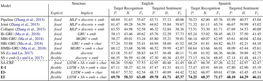
Model Structure English Spanish

Target Recognition Targeted Sentiment Target Recognition Targeted Sentiment

Explicit Implicit P. R. F1 P. R. F1 P. R. F1 P. R. F1

Pipeline (Zhang et al.,2015) fixfixed MLP+discrete + emb 60.69 51.63 55.67 43.71 37.12 40.06 70.23 62.00 65.76 45.99 40.57 43.04 Joint (Zhang et al.,2015) fixfixed MLP+discrete + emb 61.47 49.28 54.59 44.62 35.84 39.67 71.32 61.11 65.74 46.67 39.99 43.02 Collapse (Zhang et al.,2015) fixfixed MLP+discrete + emb 63.55 44.98 52.58 46.32 32.84 38.36 73.51 53.30 61.71 47.69 34.53 40.00

Bi-GRU (Ma et al.,2018) fixfixed GRU+emb 58.13 43.46 49.62 45.76 32.29 37.73 65.24 53.02 58.45 46.33 37.50 41.45

MBi-GRU (Ma et al.,2018) fixfixed MGRU+emb 58.27 49.01 53.24 45.80 35.21 39.81 66.14 60.07 62.95 45.61 40.04 42.64

HBi-GRU (Ma et al.,2018) fixfixed GRU+emb + char 57.24 53.88 55.41 44.94 38.60 41.52 68.24 61.81 64.82 46.53 42.21 44.18 HMBi-GRU (Ma et al.,2018) fixfixed MGRU+emb + char 60.12 53.68 56.98 46.52 39.99 42.87 68.64 63.66 66.01 48.09 43.44 45.61

SS (Li and Lu,2017) flexible discrete 63.18 51.67 56.83 44.57 36.48 40.11 71.49 61.92 66.36 46.06 39.89 42.75

SS +emb(Li and Lu,2017) flexible discrete + emb 66.35 56.59 61.08 47.30 40.36 43.55 73.13 64.34 68.45 47.14 41.48 44.13

SA-CRF fixfixed LSTM+SA+emb + char 60.26 55.60 57.53 42.95 40.46 41.45 68.47 66.39 67.26 42.22 42.97 42.47

E-I flexible LSTM+SA+emb + char 67.11 58.37 62.34 47.47 41.31 44.11 73.47 65.91 69.44 47.80 42.90 45.19

EI- flexible LSTM+emb + char 68.67 57.52 62.54 48.73 40.89 44.42 72.62 66.97 69.61 47.06 43.45 45.14

EI flexible LSTM+SA+emb + char 69.70 58.33 63.48 49.78 41.71 45.37 74.25 68.37 71.17 48.10 44.29 46.11

Table 2: Main Results. fixedstands for chain structures andflexiblefor latent structures. discrete,embandchar denote discrete features, word embeddings and character embeddings respectively.SArepresents self-attention.

causing the model to learn less explicit struc-tural information in the output space.

• EI-is a weaker version ofEI. Such a model removes the self-attention from EI, causing the model to learn less expressive implicit structures in the input space.

4 Results and Discussion

4.1 Main Results

The main results are presented in Table 2, where explicit structures as well as implicit structures are indicated for each model for clear comparisons.

In general, our model EI outperforms all the baselines. Specifically, it outperforms the strongest baselineEI-significantly withp <0.01 on the English and Spanish datasets in terms ofF1 scores5. Note thatEI-which models flexible ex-plicit structures and less imex-plicit structural infor-mation, achieves better performance than most of the baselines, indicating flexible explicit structures contribute a lot to the performance boost.

Now let us take a closer look at the differences based on detailed comparisons. First of all, we compare our model EI with the work proposed byZhang et al.(2015). The Pipeline model (based on CRF) as well as Joint and Collapse models (based on SSVM) in their work capturefixed ex-plicit structures. Such two models rely on multi-layer perceptron (MLP) to obtain the local context features for implicit structures. These two models do not put much effort to capture better explicit structures and implicit structures. Our model EI

(and evenEI-) outperforms these two models sig-nificantly. We also compare our work with

mod-5_{We have conducted significance test using the bootstrap}

resampling method (Koehn,2004).

els in Ma et al. (2018), which also capture fixed explicit structures. Such models leverage ent GRUs (single-layer or multi-layer) and differ-ent input features (word embeddings and charac-ter representations) to learn betcharac-ter contextual fea-tures. Their best result by HMBi-GRU is obtained with multi-layer GRU with word embeddings and character embeddings. As we can see, our model

EI outperforms HMBi-GRU under all evaluation metrics. On the English data, EI obtains 6.50 higherF1score and2.50higherF1score on target recognition and targeted sentiment respectively. On Spanish,EIobtains 5.16 higherF1 score and 0.50higherF1score on target recognition and tar-geted sentiment respectively. Notably, compared with HMBi-GRU, evenEI-capturing the flexible explicit structures achieves better performance on most of metrics and obtains the comparable re-sults in terms of precision andF1 score on Span-ish. Since both EI and EI- models attempt to capture the flexible explicit structures, the com-parisons above imply the importance of modeling suchflexibleexplicit structures in the output space.

We also compare EI with E-I. The difference between these two models is thatE-Iremoves the BMES sub-tags. Such a model captures less ex-plicit structural information in the output space. We can see thatEIoutperformsE-I. Such results show that adoptingBMES sub-tags in the output space to capture explicit structural information is beneficial.

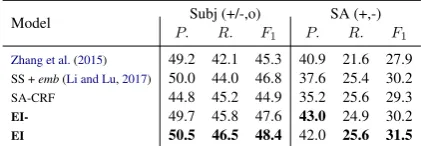
Model Subj (+/-,o) SA (+,-)

P. R. F1 P. R. F1

Zhang et al.(2015) 49.2 42.1 45.3 40.9 21.6 27.9

SS +emb(Li and Lu,2017) 50.0 44.0 46.8 37.6 25.4 30.2

SA-CRF 44.8 45.2 44.9 35.2 25.6 29.3

EI- 49.7 45.8 47.6 43.0 24.9 30.2

EI 50.5 46.5 48.4 42.0 25.6 31.5

Table 3: Results on subjectivity as well as non-neutral sentiment analysis on the Spanish dataset. Subj(+/-,o): subjectivity for all polarities. SA(+,-): sentiment anal-ysis for non-neutral polarities.

which model output representations as latent vari-ables. We can see thatEIoutperforms SA-CRF on all the metrics. Such a comparison also implies the importance of capturingflexibleexplicit structures in the output space.

Next, we focus on the comparisons with SS (Li and Lu, 2017) and SS +emb (Li and Lu, 2017). Such two models as well as our models all capture the flexible explicit structures. As for the differ-ence, both two SS models rely on hand-crafted dis-crete features to capture implicit structures, while our modelEI andEI-learn better implicit struc-tures by LSTM and self-attention. Furthermore, our models only require word embeddings and character embeddings as the input to our neural architecture to model rich implicit structures, lead-ing to a comparatively simpler and more straight-forward design. The comparison here suggests that LSTM and self-attention neural networks are able to capture better implicit structures than hand-crafted features.

Finally, we compare EI withEI-. We can see that the F1 scores of targeted sentiment for both English and Spanish produced byEIare0.95and 0.97 points higher than EI-. The main differ-ence here is that EI makes use of self-attention to capture richer implicit structures between each target phrase and all words in the complete sen-tence. The comparisons here indicate the impor-tance of capturing rich implicit structures using self-attention on this task.

Robustness

Overall, all these comparisons above based on em-pirical results show the importance of capturing bothflexibleexplicit structures in the output space and rich implicit structures by LSTM and self-attention in the input space.

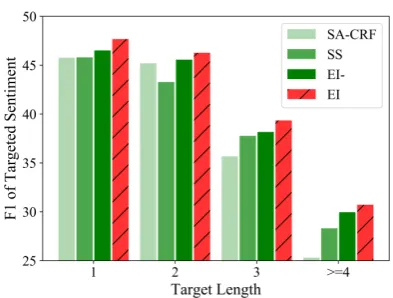
We analyze the model robustness by assessing the performance on the targeted sentiment for

tar-gets of different lengths. For both English and Spanish, we group targets into 4 categories respec-tively, namely length of 1, 2, 3 and ≥ 4. Fig-ure5 reports the F1 scores of targeted sentiment for such 4 groups on Spanish6. As we can seeEI

outperforms all the baselines on all groups. Furthermore, following the comparisons inZhang et al.(2015), we also measure the preci-sion, recall andF1of subjectivity and non-neutral polarities on the Spanish dataset. Results are reported in Table 37. The subjectivity measures whether a target phrase expresses an opinion or not according to Liu (2010). Comparing with the best-performing system’s results reported in Zhang et al. (2015) and Li and Lu (2017), our model EI can achieve higher F1 scores on subjectivity and non-neutral polarities.

Error Analysis

We conducted error analysis for our main model

EI. We calculate F1 scores based on the partial match instead of exact match. TheF1 scores for target partial match is76.04and83.82for English and Spanish respectively. We compare these two numbers against 63.48 and 71.17 which are the

F1 scores based on exact match. This compar-ison indicates that boundaries of many predicted targets do not match exactly with those of the cor-rect targets. Furthermore, we investigate the er-rors caused by incorrect sentiment polarities. We found that the major type of errors is to incorrectly predict positive targets as neutral targets. Such er-rors contribute 64% and 36% of total errors for English and Spanish respectively. We believe they are mainly caused by challenging expressions in the tweet input text. Such challenging expressions such as “below expectations” are very sparse in the data, which makes effective learning for such phrases difficult.

4.2 Effect of Implicit Structures

In order to understand whether the implicit struc-tures are truly making contributions in terms of the overall performance, we compare the perfor-mance among four models: EIandEI-as well as two variantsEI(i:MLP) andEI(i:Identity) (where iindicates the implicit structure). Such two vari-ants replace the implicit structure by other compo-nents:

6

See the English results in the supplementary material.

Model

English Spanish

Target Recognition Targeted Sentiment Target Recognition Targeted Sentiment

Prec. Rec. F1 Prec. Rec. F1 Prec. Rec. F1 Prec. Rec. F1

EI 69.70 58.33 63.48 49.78 41.71 45.37 74.25 68.37 71.17 48.10 44.29 46.11 EI(i:MLP) 64.47 56.58 60.20 46.23 40.48 43.12 70.95 65.80 68.27 43.64 40.46 41.98

EI(i:Identity) 63.24 55.73 59.20 45.10 39.79 42.24 69.38 66.27 67.77 43.66 41.68 42.63

EI- 68.67 57.52 62.54 48.73 40.89 44.42 72.62 66.97 69.61 47.06 43.45 45.14

Table 4: Effect of Implicit Structures

Figure 5: Results of different lengths on Spanish

+/0 +/+ +/+

Czech Republic , Greece and Russian ... sound good

Figure 6: An example sentence in the test data.

• EI(i:MLP) replaces self-attention by multi-layer perceptron (MLP) for implicit struc-tures. Such a variant attempts to capture im-plicit structures for a target phrase towards words restricted by a window of size3 cen-tered at the two ends of the target phrase.

• EI (i:Identity) replaces self-attention by an identity layer8 as implicit structure. Such a variant attempts to capture implicit structures for a target phrase towards words at the two ends of the target phrase exactly.

Overall, those variants perform worse than EI

on all the metrics. When the self-attention is re-placed by MLP or the identity layer for implicit structures, the performance drops a lot on both target and targeted sentiment. Such two variants

EI(i:MLP) andEI(i:Identity) consider the words within a small window centered at the two ends of the target phrase, which might not be capable of capturing the desired implicit structures. The

EI-model capturing less implicit structural

infor-8_{The identity layer returns the identical input data.}

mation achieves worse results than EI, but ob-tains better results than the two variants discussed above. This comparison implies that properly cap-turing implicit structures as the complement of ex-plicit structural information is essential.

4.3 Qualitative Analysis

We present an example sentence in the test data in Figure 6, where the gold targets are in bold, the predicted targets are in the pink boxes, the gold sentiment is in blue and predicted sentiment is in red. EI makes all correct predictions for three targets. EI- predicts correct boundaries for three targets and the targeted sentiment predictions are highlighted in Figure6. As we can see,EI- incor-rectly predicts the targeted sentiment on the first target as neural (0). The first target here is far from the sentiment expression “sound good” which is not in the first sentiment span, making EI- not capable of capturing such a sentiment expression. This qualitative analysis helps us to better under-stand the importance to capture implicit structures using both LSTM and self-attention.

4.4 Additional Experiments

We also conducted experiments on multi-lingual Restaurant datasets from SemEval 2016 Task 5 (Pontiki et al.,2016), where aspect target phrases and aspect sentiments are provided. 9 We regard each aspect target phrase as a target and assign such a target with the corresponding aspect sen-timent polarity in the data. Note that we remove all the instances which contain no targets in the training data. Following the main experiment, we split10% of training data as development set for the selection of the best model during training.

We report the F1 scores of target and targeted sentiment for English, Dutch and Russian10 re-spectively in Table 5. The results show that EI

9

See the supplementary material for data statistics.

10_{We use the pretrained embedding for Dutch and}

Russian from https://github.com/Kyubyong/

achieves the best performance. The performance of SS (Li and Lu,2017) is much worse on Rus-sian due to the inability of discrete features in SS to capture the complex morphology in Russian.

5 Related Work

We briefly survey the research efforts on two types of TSA tasks mentioned in the introduction. Note that TSA is related to aspect sentiment analysis which is to determine the sentiment polarity given a target and an aspect describing a property of re-lated topics.

Predicting sentiment for a given target

Such a task is typically solved by leveraging sen-tence structural information, such as syntactic trees (Dong et al.,2014), dependency trees (Wang et al.,2016) as well as surrounding context based on LSTM (Tang et al.,2016a), GRU (Zhang et al.,

2016) or CNN (Xue and Li,2018). Another line of works leverage self-attention (Liu and Zhang,

2017) or memory networks (Tang et al.,2016b) to encode rich global context information.Wang and Lu(2018) adopted the segmental attention (Kong et al.,2016) to model the important text segments to compute the targeted sentiment. Wang et al.

(2018) studied the issue that the different combi-nations of target and aspect may result in differ-ent sdiffer-entimdiffer-ent polarity. They proposed a model to distinguish such different combinations based on memory networks to produce the representation for aspect sentiment classification.

Jointly predicting targets and their associated sentiment

Such a joint task is usually regarded as sequence labeling problem. Mitchell et al. (2013) intro-duced the task of open domain targeted sentiment analysis. They proposed several models based on CRF such as the pipeline model, the collapsed model as well as the joint model to predict both targets and targeted sentiment information. Their experiments showed that the collapsed model and the joint model could achieve better results, im-plying the benefit of the joint learning on this task.

Zhang et al. (2015) proposed an approach based on structured SVM (Taskar et al.,2005; Tsochan-taridis et al., 2005) integrating both discrete fea-tures and neural feafea-tures for this joint task.Li and Lu (2017) proposed the sentiment scope model motivated from a linguistic phenomenon to repre-sent the structure information for both the targets

Model English Dutch Russian

target sent target sent target sent

SS (Li and Lu,2017) 46.3 36.9 44.6 33.4 20.2 14.5

SS +emb(Li and Lu,2017) 57.1 48.0 46.8 33.5 35.9 24.1

SA-CRF 60.8 51.4 49.7 34.0 54.2 43.4

EI- 57.7 48.2 47.2 33.7 52.8 38.9

EI 62.0 51.6 50.0 34.2 54.4 43.4

Table 5: F1 scores of targets (target) and their asso-ciated sentiment (sent) on SemEval 2016 Restaurant Dataset.

and their associated sentiment polarities. They modelled the latent sentiment scope based on CRF with latent variables, and achieved the best per-formance among all the existing works. How-ever, they did not explore much on the implicit structural information and their work mostly re-lied on hand-crafted discrete features. Ma et al.

(2018) adopted a multi-layer GRU to learn targets and sentiments jointly by producing the target tag and the sentiment tag at each position. They in-troduced a constraint forcing the sentiment tag at each position to be consistent with the target tag. However, they did not explore the explicit struc-tural information in the output space as we do in this work.

6 Conclusion and Future Work

In this work, we argue that properly modeling both explicitstructures in the output space and the im-plicitstructures in the input space are crucial for building a successful targeted sentiment analysis system. Specifically, we propose a new model that captures explicit structures with latent CRF, and uses LSTM and self-attention to capture rich implicit structures in the input space efficiently. Through extensive experiments, we show that our model is able to outperform competitive baseline models significantly, thanks to its ability to prop-erly capture both explicit and implicit structural information.

Future work includes exploring approaches to capture explicit and implicit structural information to other sentiment analysis tasks and other struc-tured prediction problems.

Acknowledgments

References

Mark Cieliebak, Jan Milan Deriu, Dominic Egger, and Fatih Uzdilli. 2017.A twitter corpus and benchmark resources for german sentiment analysis. InProc. of the Fifth International Workshop on Natural Lan-guage Processing for Social Media.

Trinh Do, Thierry Arti, et al. 2010. Neural conditional random fields. InProc. of AISTATS.

Li Dong, Furu Wei, Chuanqi Tan, Duyu Tang, Ming Zhou, and Ke Xu. 2014. Adaptive recursive neural network for target-dependent twitter sentiment clas-sification. InProc. of ACL.

Feifan Fan, Yansong Feng, and Dongyan Zhao. 2018. Multi-grained attention network for aspect-level sentiment classification. InProc. of EMNLP.

Xavier Glorot and Yoshua Bengio. 2010. Understand-ing the difficulty of trainUnderstand-ing deep feedforward neural networks. InProc. of AISTATS.

Ruidan He, Wee Sun Lee, Hwee Tou Ng, and Daniel Dahlmeier. 2018. Effective attention modeling for aspect-level sentiment classification. In Proc. of COLING.

Diederik P Kingma and Jimmy Ba. 2014. Adam: A method for stochastic optimization. InProc. of ICLR.

Philipp Koehn. 2004. Statistical significance tests for machine translation evaluation. InProc. of EMNLP.

Lingpeng Kong, Chris Dyer, and Noah A Smith. 2016. Segmental recurrent neural networks. In Proc. of ICLR.

John Lafferty, Andrew McCallum, and Fernando CN Pereira. 2001. Conditional random fields: Prob-abilistic models for segmenting and labeling se-quence data. InProc. of ICML.

Guillaume Lample, Miguel Ballesteros, Sandeep Sub-ramanian, Kazuya Kawakami, and Chris Dyer. 2016. Neural architectures for named entity recognition. InProc. of NAACL.

Hao Li and Wei Lu. 2017. Learning latent sentiment scopes for entity-level sentiment analysis. InProc. of AAAI.

Nan Li and Desheng Dash Wu. 2010. Using text min-ing and sentiment analysis for online forums hotspot detection and forecast. Decision support systems, 48(2).

Bing Liu. 2010. Sentiment analysis and subjectivity. Handbook of natural language processing.

Jiangming Liu and Yue Zhang. 2017. Attention mod-eling for targeted sentiment. InProc. of EACL.

Dehong Ma, Sujian Li, and Houfeng Wang. 2018.Joint learning for targeted sentiment analysis. InProc. of EMNLP.

Margaret Mitchell, Jacqueline Aguilar, Theresa Wil-son, and Benjamin Van Durme. 2013.Open domain targeted sentiment. InProc. of EMNLP.

Alvaro Ortigosa, Jos´e M Mart´ın, and Rosa M Carro. 2014. Sentiment analysis in facebook and its appli-cation to e-learning. Computers in Human Behav-ior.

Bo Pang and Lillian Lee. 2008. Opinion mining and sentiment analysis.Foundations and trends in infor-mation retrieval, 2(1-2).

Adam Paszke, Sam Gross, Soumith Chintala, Gre-gory Chanan, Edward Yang, Zachary DeVito, Zem-ing Lin, Alban Desmaison, Luca Antiga, and Adam Lerer. 2017. Automatic differentiation in pytorch. InProc. of NIPS.

Jian Peng, Liefeng Bo, and Jinbo Xu. 2009. Condi-tional neural fields. InProc. of NIPS.

Jeffrey Pennington, Richard Socher, and Christo-pher D. Manning. 2014. Glove: Global vectors for word representation. InProc. of EMNLP.

Maria Pontiki, Dimitris Galanis, Haris Papageor-giou, Ion Androutsopoulos, Suresh Manandhar, Mo-hammed AL-Smadi, Mahmoud Al-Ayyoub, Yanyan Zhao, Bing Qin, Orph´ee De Clercq, et al. 2016. Semeval-2016 task 5: Aspect based sentiment anal-ysis. InProc. of SemEval.

Jasmina Smailovi´c, Miha Grˇcar, Nada Lavraˇc, and Martin ˇZnidarˇsiˇc. 2013. Predictive sentiment analysis of tweets: A stock market application. In Human-Computer Interaction and Knowledge Discovery in Complex, Unstructured, Big Data. Springer.

Duyu Tang, Bing Qin, Xiaocheng Feng, and Ting Liu. 2016a. Effective LSTMs for target-dependent senti-ment classification. InProc. of COLING.

Duyu Tang, Bing Qin, and Ting Liu. 2016b. Aspect level sentiment classification with deep memory net-work. InProc. of EMNLP.

Ben Taskar, Vassil Chatalbashev, Daphne Koller, and Carlos Guestrin. 2005. Learning structured predic-tion models: A large margin approach. InProc. of ICML.

Ioannis Tsochantaridis, Thorsten Joachims, Thomas Hofmann, and Yasemin Altun. 2005. Large mar-gin methods for structured and interdependent out-put variables.Journal of machine learning research, 6(Sep):1453–1484.

Bailin Wang and Wei Lu. 2018. Learning latent opin-ions for aspect-level sentiment classification. In Proc. of AAAI.

Wenya Wang, Sinno Jialin Pan, Daniel Dahlmeier, and Xiaokui Xiao. 2016. Recursive neural conditional random fields for aspect-based sentiment analysis. InProc. of EMNLP.

Wei Xue and Tao Li. 2018. Aspect based sentiment analysis with gated convolutional networks. InProc. of ACL.

Meishan Zhang, Yue Zhang, and Duy-Tin Vo. 2015. Neural networks for open domain targeted senti-ment. InProc. of EMNLP.