Estimating Strictly Piecewise Distributions
Jeffrey Heinz
University of Delaware Newark, Delaware, USA
James Rogers
Earlham College Richmond, Indiana, USA
Abstract
Strictly Piecewise (SP) languages are a subclass of regular languages which en-code certain kinds of long-distance de-pendencies that are found in natural lan-guages. Like the classes in the Chom-sky and Subregular hierarchies, there are many independently converging character-izations of the SP class (Rogers et al., to appear). Here we define SP distributions and show that they can be efficiently esti-mated from positive data.
1 Introduction
Long-distance dependencies in natural language are of considerable interest. Although much at-tention has focused on long-distance dependencies which are beyond the expressive power of models with finitely many states (Chomsky, 1956; Joshi, 1985; Shieber, 1985; Kobele, 2006), there are some long-distance dependencies in natural lan-guage which permit finite-state characterizations. For example, although it is well-known that vowel and consonantal harmony applies across any ar-bitrary number of intervening segments (Ringen, 1988; Bakovi´c, 2000; Hansson, 2001; Rose and Walker, 2004) and that phonological patterns are regular (Johnson, 1972; Kaplan and Kay, 1994), it is less well-known that harmony patterns are largely characterizable by the Strictly Piecewise languages, a subregular class of languages with independently-motivated, converging characteri-zations (see Heinz (2007, to appear) and especially Rogers et al. (2009)).
As shown by Rogers et al. (to appear), the Strictly Piecewise (SP) languages, which make distinctions on the basis of (potentially) discon-tiguous subsequences, are precisely analogous to the Strictly Local (SL) languages (McNaughton and Papert, 1971; Rogers and Pullum, to appear),
which make distinctions on the basis of contigu-ous subsequences. The Strictly Local languages are the formal-language theoretic foundation for n-gram models (Garcia et al., 1990), which are widely used in natural language processing (NLP) in part because such distributions can be estimated from positive data (i.e. a corpus) (Jurafsky and Martin, 2008). N-gram models describe prob-ability distributions over all strings on the basis of the Markov assumption (Markov, 1913): that the probability of the next symbol only depends on the previous contiguous sequence of length n−1. From the perspective of formal language theory, these distributions are perhaps properly called Strictly k-Local distributions (SLk) where
k=n. It is well-known that one limitation of the Markov assumption is its inability to express any kind of long-distance dependency.
This paper defines Strictly k-Piecewise (SPk)
distributions and shows how they too can be effi-ciently estimated from positive data. In contrast with the Markov assumption, our assumption is that the probability of the next symbol is condi-tioned on the previous set of discontiguous subse-quences of length k−1 in the string. While this suggests the model has too many parameters (one for each subset of all possible subsequences), in fact the model has on the order of|Σ|k+1 parame-ters because of an independence assumption: there is no interaction between different subsequences. As a result, SP distributions are efficiently com-putable even though they condition the probabil-ity of the next symbol on the occurrences of ear-lier (possibly very distant) discontiguous subse-quences. Essentially, these SP distributions reflect a kind of long-term memory.
On the other hand, SP models have no short-term memory and are unable to make distinctions on the basis of contiguous subsequences. We do not intend SP models to replace n-gram models, but instead expect them to be used alongside of
them. Exactly how this is to be done is beyond the scope of this paper and is left for future research.
Since SP languages are the analogue of SL lan-guages, which are the formal-language theoretical foundation for n-gram models, which are widely used in NLP, it is expected that SP distributions and their estimation will also find wide applica-tion. Apart from their interest to problems in the-oretical phonology such as phonotactic learning (Coleman and Pierrehumbert, 1997; Hayes and Wilson, 2008; Heinz, to appear), it is expected that their use will have application, in conjunction with n-gram models, in areas that currently use them; e.g. augmentative communication (Newell et al., 1998), part of speech tagging (Brill, 1995), and speech recognition (Jelenik, 1997).
§2 provides basic mathematical notation. §3 provides relevant background on the subregular hi-erarchy. §4 describes automata-theoretic charac-terizations of SP languages. §5 defines SP distri-butions. §6 shows how these distributions can be efficiently estimated from positive data and pro-vides a demonstration. §7 concludes the paper.
2 Preliminaries
We start with some mostly standard notation. Σ denotes a finite set of symbols and a string over Σ is a finite sequence of symbols drawn from that set. Σk, Σ≤k, Σ≥k, and Σ∗ denote all
strings over this alphabet of length k, of length less than or equal to k, of length greater than or equal to k, and of any finite length, respec-tively. ǫ denotes the empty string. |w| denotes the length of string w. The prefixes of a string ware Pfx(w) ={v:∃u∈Σ∗such thatvu=w}. When discussing partial functions, the notation↑
and ↓indicates that the function is undefined, re-spectively is defined, for particular arguments.
A language L is a subset ofΣ∗. A stochastic
language Dis a probability distribution over Σ∗. The probabilityp of wordwwith respect to Dis writtenP rD(w) =p. Recall that all distributions Dmust satisfyP
w∈Σ∗P rD(w) = 1. IfLis
lan-guage thenP rD(L) =P
w∈LP rD(w).
A Deterministic Finite-state Automaton (DFA) is a tuple M = hQ,Σ, q0, δ, Fi where Q is the
state set, Σ is the alphabet, q0 is the start state,
δ is a deterministic transition function with do-main Q ×Σ and codomain Q, F is the set of accepting states. Let dˆ : Q × Σ∗ → Q be the (partial) path function of M, i.e., dˆ(q, w)
is the (unique) state reachable from state q via the sequence w, if any, or dˆ(q, w)↑ other-wise. The language recognized by a DFA M is L(M)def={w∈Σ∗ |dˆ(q0, w)↓ ∈F}.
A state is useful iff for allq ∈ Q, there exists w ∈ Σ∗ such that δ(q0, w) = q and there exists
w ∈ Σ∗ such that δ(q, w) ∈ F. Useless states
are not useful. DFAs without useless states are trimmed.
Two stringsw and v over Σare distinguished by a DFA Miff dˆ(q0, w) 6= ˆd(q0, v). They are
Nerode equivalent with respect to a language L if and only if wu ∈ L ⇐⇒ vu ∈ L for all u ∈ Σ∗. All DFAs which recognize L must distinguish strings which are inequivalent in this sense, but no DFA recognizing Lnecessarily dis-tinguishes any strings which are equivalent. Hence the number of equivalence classes of strings over Σ modulo Nerode equivalence with respect toL gives a (tight) lower bound on the number of states required to recognizeL.
A DFA is minimal if the size of its state set is minimal among DFAs accepting the same lan-guage. The product of n DFAs M1. . .Mn is
given by the standard construction over the state spaceQ1×. . .×Qn(Hopcroft et al., 2001).
A Probabilistic Deterministic Finite-state Automaton (PDFA) is a tuple
M = hQ,Σ, q0, δ, F, Ti where Q is the state
set, Σ is the alphabet, q0 is the start state, δ is
a deterministic transition function, F and T are the final-state and transition probabilities. In particular, T : Q×Σ → R+ and F : Q → R+ such that
for allq∈Q, F(q) +X
a∈Σ
T(q, a) = 1. (1)
Like DFAs, for allw ∈ Σ∗, there is at most one
state reachable fromq0. PDFAs are typically
rep-resented as labeled directed graphs as in Figure 1.
A PDFA M generates a stochastic language
DM. If it exists, the (unique) path for a wordw=
a0. . . ak belonging to Σ∗ through a PDFA is a
sequence h(q0, a0),(q1, a1), . . . ,(qk, ak)i, where
qi+1 =δ(qi, ai). The probability a PDFA assigns
A:2/10 b : 2 / 1 0 c : 3 / 1 0
B:4/9 a : 3 / 1 0
[image:3.595.335.525.84.145.2]a : 2 / 9 b:2/9 c:1/9
Figure 1: A picture of a PDFA with states labeled A and B. The probabilities of T and F are located to the right of the colon.
it exists, and zero otherwise.
P rDM(w) =
k Y i=1
T(qi−1, ai−1) !
·F(qk+1) (2)
ifdˆ(q0, w)↓and 0 otherwise
A probability distribution is regular deterministic iff there is a PDFA which generates it.
The structural components of a PDFA M are its states Q, its alphabet Σ, its transitions δ, and its initial state q0. By structure of a PDFA, we mean its structural components. Each PDFA M
defines a family of distributions given by the pos-sible instantiations of T and F satisfying Equa-tion 1. These distribuEqua-tions have|Q|·(|Σ|+ 1) in-dependent parameters (since for each state there are|Σ|possible transitions plus the possibility of finality.)
We define the product of PDFA in terms of co-emission probabilities (Vidal et al., 2005a). Definition 1 LetAbe a vector of PDFAs and let
|A| = n. For each 1 ≤ i ≤ n let Mi =
hQi,Σ, q0i, δi, Fi, Tii be theith PDFA inA. The
probability thatσis co-emitted fromq1, . . . , qnin
Q1, . . . , Qn, respectively, is
CT(hσ, q1 . . . qni) = n Y i=1
Ti(qi, σ).
Similarly, the probability that a word simultane-ously ends atq1 ∈Q1 . . . qn∈Qnis
CF(hq1 . . . qni) =
n Y i=1
Fi(qi).
ThenN
A=hQ,Σ, q0, δ, F, Tiwhere
1. Q, q0,andδare defined as with DFA product.
2. For all hq1 . . . qni ∈ Q, let
Z(hq1 . . . qni) =
CF(hq1 . . . qni) + X σ∈Σ
CT(hσ, q1 . . . qni)
be the normalization term; and
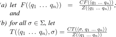
(a) let F(hq1 . . . qni) = CF(hq1... q
ni)
Z(hq1... qni) ;
and
(b) for allσ ∈Σ, let
T(hq1 . . . qni, σ) = CT(hσ, q1... q
ni)
Z(hq1... qni)
In other words, the numerators ofT andF are de-fined to be the co-emission probabilities (Vidal et al., 2005a), and division byZensures thatM de-fines a well-formed probability distribution. Sta-tistically speaking, the co-emission product makes an independence assumption: the probability ofσ being co-emitted fromq1, . . . , qnis exactly what
one expects if there is no interaction between the individual factors; that is, between the probabil-ities of σ being emitted from any qi. Also note
order of product is irrelevant up to renaming of the states, and so therefore we also speak of tak-ing the product of a set of PDFAs (as opposed to an ordered vector).
Estimating regular deterministic distributions is well-studied problem (Vidal et al., 2005a; Vidal et al., 2005b; de la Higuera, in press). We limit dis-cussion to cases when the structure of the PDFA is known. Let S be a finite sample of words drawn from a regular deterministic distribution D. The problem is to estimate parameters T andF ofM
so thatDMapproachesD. We employ the
widely-adopted maximum likelihood (ML) criterion for this estimation.
( ˆT ,Fˆ) = argmax
T,F
Y w∈S
P rM(w) !
(3)
It is well-known that if D is generated by some PDFAM′with the same structural components as
M, then optimizing the ML estimate guarantees that DM approaches D as the size of S goes to
infinity (Vidal et al., 2005a; Vidal et al., 2005b; de la Higuera, in press).
The optimization problem (3) is simple for de-terministic automata with known structural com-ponents. Informally, the corpus is passed through the PDFA, and the paths of each word through the corpus are tracked to obtain counts, which are then normalized by state. LetM= hQ,Σ, δ, q0, F, Ti
be the PDFA whose parameters F and T are to be estimated. For all states q ∈ Qand symbolsa ∈
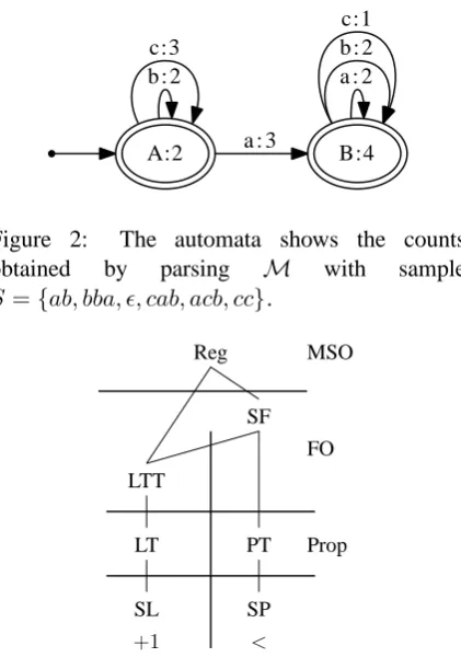
A:2 b : 2 c:3
B:4 a : 3
[image:4.595.77.288.66.372.2]a : 2 b : 2 c:1
Figure 2: The automata shows the counts obtained by parsing M with sample S ={ab, bba, ǫ, cab, acb, cc}.
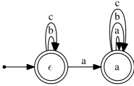
SL SP
LT PT
LTT
SF
FO
Reg MSO
Prop
+1 <
Figure 3: Parallel Sub-regular Hierarchies.
number of times stateqis encountered in the pars-ing ofS. Similarly, the ML estimation ofF(q)is obtained by calculating the relative frequency of stateq being final with stateq being encountered in the parsing ofS. For both cases, the division is normalizing; i.e. it guarantees that there is a well-formed probability distribution at each state. Fig-ure 2 illustrates the counts obtained for a machine
M with sample S = {ab, bba, ǫ, cab, acb, cc}.1 Figure 1 shows the PDFA obtained after normaliz-ing these counts.
3 Subregular Hierarchies
Within the class of regular languages there are dual hierarchies of language classes (Figure 3), one in which languages are defined in terms of their contiguous substrings (up to some lengthk, known as k-factors), starting with the languages that are Locally Testable in the Strict Sense (SL), and one in which languages are defined in terms of their not necessarily contiguous subsequences, starting with the languages that are Piecewise
1Technically, this acceptor is neither a simple DFA or
PDFA; rather, it has been called a Frequency DFA. We do not formally define them here, see (de la Higuera, in press).
Testable in the Strict Sense (SP). Each language class in these hierarchies has independently mo-tivated, converging characterizations and each has been claimed to correspond to specific, fundamen-tal cognitive capabilities (McNaughton and Pa-pert, 1971; Brzozowski and Simon, 1973; Simon, 1975; Thomas, 1982; Perrin and Pin, 1986; Garc´ıa and Ruiz, 1990; Beauquier and Pin, 1991; Straub-ing, 1994; Garc´ıa and Ruiz, 1996; Rogers and Pul-lum, to appear; Kontorovich et al., 2008; Rogers et al., to appear).
Languages in the weakest of these classes are defined only in terms of the set of factors (SL) or subsequences (SP) which are licensed to oc-cur in the string (equivalently the complement of that set with respect to Σ≤k, the forbidden
fac-tors or forbidden subsequences). For example, the set containing the forbidden 2-factors{ab, ba} de-fines a Strictly 2-Local language which includes all strings except those with contiguous substrings
{ab, ba}. Similarly since the parameters of n-gram models (Jurafsky and Martin, 2008) assign probabilities to symbols given the preceding con-tiguous substrings up to lengthn−1, we say they describe Strictlyn-Local distributions.
These hierarchies have a very attractive model-theoretic characterization. The Locally Testable (LT) and Piecewise Testable languages are exactly those that are definable by propositional formulae in which the atomic formulae are blocks of sym-bols interpreted factors (LT) or subsequences (PT) of the string. The languages that are testable in the strict sense (SL and SP) are exactly those that are definable by formulae of this sort restricted to con-junctions of negative literals. Going the other way, the languages that are definable by First-Order for-mulae with adjacency (successor) but not prece-dence (less-than) are exactly the Locally Thresh-old Testable (LTT) languages. The Star-Free lan-guages are those that are First-Order definable with precedence alone (adjacency being FO defin-able from precedence). Finally, by extending to Monadic Second-Order formulae (with either sig-nature, since they are MSO definable from each other), one obtains the full class of Regular lan-guages (McNaughton and Papert, 1971; Thomas, 1982; Rogers and Pullum, to appear; Rogers et al., to appear).
subse-quence relation, which is a partial order onΣ∗:
w⊑v⇐⇒def w=εorw=σ1· · ·σnand
(∃w0, . . . , wn∈Σ∗)[v=w0σ1w1· · ·σnwn].
in which case we saywis a subsequence ofv. Forw∈Σ∗, let
Pk(w)
def
={v∈Σk |v⊑w}and
P≤k(w)
def
={v∈Σ≤k|v⊑w},
the set of subsequences of length k, respectively length no greater than k, of w. Let Pk(L) and
P≤k(L) be the natural extensions of these to sets
of strings. Note that P0(w) ={ε}, for allw∈Σ∗,
that P1(w)is the set of symbols occurring inwand
that P≤k(L)is finite, for allL⊆Σ∗.
Similar to the Strictly Local languages, Strictly Piecewise languages are defined only in terms of the set of subsequences (up to some length k) which are licensed to occur in the string.
Definition 2 (SPkGrammar, SP) A SPk
gram-mar is a pair G = hΣ, Gi where G ⊆ Σk. The
language licensed by a SPkgrammar is
L(G)def={w∈Σ∗ |P≤k(w)⊆P≤k(G)}.
A language is SPk iff it is L(G) for some SPk
grammarG. It is SP iff it is SPkfor somek.
This paper is primarily concerned with estimat-ing Strictly Piecewise distributions, but first we examine in greater detail properties of SP lan-guages, in particular DFA representations.
4 DFA representations of SP Languages
Following Sakarovitch and Simon (1983), Lothaire (1997) and Kontorovich, et al. (2008), we call the set of strings that contain w as a subsequence the principal shuffle ideal2ofw:
SI(w) ={v ∈Σ∗|w⊑v}.
The shuffle ideal of a set of strings is defined as
SI(S) =∪w∈SSI(w)
Rogers et al. (to appear) establish that the SP lan-guages have a variety of characteristic properties.
Theorem 1 The following are equivalent:3
2Properly SI(w)is the principal ideal generated by{w}
wrt the inverse of⊑.
3For a complete proof, see Rogers et al. (to appear). We
only note that 5 implies 1 by DeMorgan’s theorem and the fact that every shuffle ideal is finitely generated (see also Lothaire (1997)).
1 b c
2 a
[image:5.595.347.488.60.137.2]b c
Figure 4: The DFA representation of SI(aa).
1. L=T
w∈S[SI(w)], Sfinite,
2. L∈SP
3. (∃k)[P≤k(w)⊆P≤k(L)⇒w∈L],
4. w ∈ Landv ⊑ w ⇒ v ∈ L (L is subse-quence closed),
5. L =SI(X), X ⊆ Σ∗ (Lis the complement of a shuffle ideal).
The DFA representation of the complement of a shuffle ideal is especially important.
Lemma 1 Let w ∈ Σk, w = σ
1· · ·σk,
and MSI(w) = hQ,Σ, q0, δ, Fi, where Q = {i|1≤i≤k}, q0 = 1, F = Q and for all
qi∈Q, σ∈Σ:
δ(qi, σ) =
qi+1 ifσ=σiandi < k, ↑ ifσ=σiandi=k,
qi otherwise.
ThenMSI(w)is a minimal, trimmed DFA that
rec-ognizes the complement of SI(w), i.e., SI(w) = L(MSI(w)).
Figure 4 illustrates the DFA representation of the complement of SI(aa)withΣ ={a, b, c}. It is easy to verify that the machine in Figure 4 accepts all and only those words which do not contain an aasubsequence.
For any SPk language L = L(hΣ, Gi) 6= Σ∗,
the first characterization (1) in Theorem 1 above yields a non-deterministic finite-state representa-tion ofL, which is a setAof DFA representations of complements of principal shuffle ideals of the elements ofG. The trimmed automata product of this set yields a DFA, with the properties below (Rogers et al., to appear).
Lemma 2 LetMbe a trimmed DFA recognizing a SPk language constructed as described above.
Then:
a b
c
b
c b
a
c
a
b b
c
b
b a
b
ǫ ǫ,a
ǫ,b
ǫ,c
ǫ,a,b
ǫ,b,c ǫ,a,c
[image:6.595.75.297.56.234.2]ǫ,a,b,c
Figure 5: The DFA representation of the of the SP language given by G = h{a, b, c},{aa, bc}i. Names of the states reflect subsets of subse-quences up to length 1 of prefixes of the language. Note this DFA is trimmed, but not minimal.
2. For all q1, q2 ∈ Qand σ ∈ Σ, if dˆ(q1, σ)↑
and dˆ(q1, w) = q2 for some w ∈ Σ∗ then
ˆ
d(q2, σ)↑. (Missing edges propagate down.)
Figure 5 illustrates with the DFA representa-tion of the of the SP2 language given by G = h{a, b, c},{aa, bc}i. It is straightforward to ver-ify that this DFA is identical (modulo relabeling of state names) to one obtained by the trimmed prod-uct of the DFA representations of the complement of the principal shuffle ideals ofaaandbc, which are the prohibited subsequences.
States in the DFA in Figure 5 correspond to the subsequences up to length 1 of the prefixes of the language. With this in mind, it follows that the DFA of Σ∗ = L(Σ,Σk) has states which
corre-spond to the subsequences up to length k−1 of the prefixes ofΣ∗. Figure 6 illustrates such a DFA
whenk= 2andΣ ={a, b, c}.
In fact, these DFAs reveal the differences be-tween SP languages and PT languages: they are exactly those expressed in Lemma 2. Within the state space defined by the subsequences up to lengthk−1of the prefixes of the language, if the conditions in Lemma 2 are violated, then the DFAs describe languages that are PT but not SP. Pictori-ally,P T2languages are obtained by arbitrarily
re-moving arcs, states, and the finality of states from the DFA in Figure 6, andSP2ones are obtained by
non-arbitrarily removing them in accordance with Lemma 2. The same applies straightforwardly for anyk(see Definition 3 below).
a b
c
a b
c
b a
c
c
a b
a b
c
a
c b
b c
a
a b c
ǫ ǫ,a
ǫ,b
ǫ,c
ǫ,a,b
ǫ,b,c
ǫ,a,c
ǫ,a,b,c
Figure 6: A DFA representation of the of the SP2
language given by G = h{a, b, c},Σ2i. Names of the states reflect subsets of subsequences up to length 1 of prefixes of the language. Note this DFA is trimmed, but not minimal.
5 SP Distributions
In the same way that SL distributions (n-gram models) generalize SL languages, SP distributions generalize SP languages. Recall that SP languages are characterizable by the intersection of the com-plements of principal shuffle ideals. SP distribu-tions are similarly characterized.
We begin with Piecewise-Testable distributions.
Definition 3 A distribution D is k-Piecewise
Testable (writtenD ∈ PTDk)
def
⇐⇒ Dcan be de-scribed by a PDFAM=hQ,Σ, q0, δ, F, Tiwith
1. Q={P≤k−1(w) :w∈Σ∗}
2. q0 =P≤k−1(ǫ)
3. For all w ∈ Σ∗ and all σ ∈ Σ,
δ(P≤k−1(w), a) =P≤k−1(wa)
4. F andT satisfy Equation 1.
[image:6.595.308.533.58.285.2]structure of a PDFA which describes a PT2
distri-bution as long as the assigned probabilities satisfy Equation 1.
The following lemma follows directly from the finite-state representation of PTkdistributions.
Lemma 3 Let D belong to PTDk and let M = hQ,Σ, q0, δ, F, Tibe a PDFA representing D
de-fined according to Definition 3.
P rD(σ1. . . σn) =T(P≤k−1(ǫ), σ1)·
Y 2≤i≤n
T(P≤k−1(σ1. . . σi−1), σi) (4)
· F(P≤k−1(w))
PTkdistributions have2|Σ|
k−1
(|Σ|+1)parameters (since there are2|Σ|k−1 states and|Σ|+ 1possible events, i.e. transitions and finality).
LetP r(σ | #)and P r(# | P≤k(w))denote
the probability (according to some D ∈ PTDk)
that a word begins with σ and ends after observ-ingP≤k(w). Then Equation 4 can be rewritten in
terms of conditional probability as
P rD(σ1. . . σn) =P r(σ1 |#)·
Y 2≤i≤n
P r(σi |P≤k−1(σ1. . . σi−1)) (5)
· P r(#| P≤k−1(w))
Thus, the probability assigned to a word depends not on the observed contiguous sequences as in a Markov model, but on observed subsequences.
Like SP languages, SP distributions can be de-fined in terms of the product of machines very sim-ilar to the complement of principal shuffle ideals.
Definition 4 Letw∈Σk−1andw=σ
1· · ·σk−1. Mw = hQ,Σ, q0, δ, F, Ti is a
w-subsequence-distinguishing PDFA (w-SD-PDFA) iff Q = Pfx(w), q0 = ǫ, for all u ∈ Pfx(w)
and eachσ∈Σ,
δ(u, σ) = uσiffuσ∈Pfx(w)and uotherwise
[image:7.595.346.484.68.156.2]andF andT satisfy Equation 1.
Figure 7 shows the structure of Ma which is almost the same as the complement of the princi-pal shuffle ideal in Figure 4. The only difference is the additional self-loop labeled aon the right-most state labeleda. Ma defines a family of dis-tributions overΣ∗, and its states distinguish those
b c
a a
a b c
ǫ
Figure 7: The structure of PDFA Ma. It is the
same (modulo state names) as the DFA in Figure 4 except for the self-loop labeledaon statea.
strings which contain a (state a) from those that do not (stateǫ). A set of PDFAs is a k-set of SD-PDFAs iff, for each w ∈ Σ≤k−1, it contains
ex-actly onew-SD-PDFA.
In the same way that missing edges propagate down in DFA representations of SP languages (Lemma 2), the final and transitional probabili-ties must propagate down in PDFA representa-tions of SPk distributions. In other words, the
fi-nal and transitiofi-nal probabilities at states further along paths beginning at the start state must be de-termined by final and transitional probabilities at earlier states non-increasingly. This is captured by defining SP distributions as a product ofk-sets of SD-PDFAs (see Definition 5 below).
While the standard product based on co-emission probability could be used for this pur-pose, we adopt a modified version of it defined fork-sets of SD-PDFAs: the positive co-emission probability. The automata product based on the positive co-emission probability not only ensures that the probabilities propagate as necessary, but also that such probabilities are made on the ba-sis of observed subsequences, and not unobserved ones. This idea is familiar fromn-gram models: the probability of σn given the immediately
pre-ceding sequence σ1. . . σn−1 does not depend on
the probability ofσngiven the other(n−1)-long
sequences which do not immediately precede it, though this is a logical possibility.
Let A be a k-set of SD-PDFAs. For each w∈ Σ≤k−1, letMw =hQ
w,Σ, q0w, δw, Fw, Twi
be thew-subsequence-distinguishing PDFA inA. The positive co-emission probability thatσ is si-multaneously emitted from statesqǫ, . . . , qufrom
SD-PDFA inAis
P CT(hσ, qǫ . . . qui) = Y qw∈hqǫ...qui
qw=w
Tw(qw, σ) (6)
Similarly, the probability that a word simultane-ously ends atnstatesqǫ ∈Qǫ, . . . , qu ∈Quis
P CF(hqǫ . . . qui) = Y qw∈hqǫ...qui
qw=w
Fw(qw) (7)
In other words, the positive co-emission proba-bility is the product of the probabilities restricted to those assigned to the maximal states in each
Mw. For example, consider a 2-set of
SD-PDFAs A with Σ = {a, b, c}. A contains four PDFAs Mǫ,Ma,Mb,Mc. Consider state q =
hǫ, ǫ, b, ci ∈N
A(this is the state labeledǫ, b, cin Figure 6). Then
CT(a, q) =Tǫ(ǫ, a)· Ta(ǫ, a)· Tb(b, a)· Tc(c, a)
but
P CT(a, q) =Tǫ(ǫ, a)· Tb(b, a)· Tc(c, a)
since in PDFAMa, the stateǫis not the maximal state.
The positive co-emission product (⊗+) is
de-fined just as with co-emission probabilities, sub-stituting PCT and PCF for CT and CF, respec-tively, in Definition 1. The definition of ⊗+ en-sures that the probabilities propagate on the basis of observed subsequences, and not on the basis of unobserved ones.
Lemma 4 Letk ≥ 1and letAbe ak-set of SD-PDFAs. Then ⊗+S defines a well-formed
proba-bility distribution overΣ∗.
Proof Since Mǫ belongs to A, it is always the case that PCT and PCF are defined. Well-formedness follows from the normalization term as in Definition 1. ⊣⊣⊣
Definition 5 A distribution Disk-Strictly
Piece-wise (writtenD ∈SPDk)
def
⇐⇒ Dcan be described by a PDFA which is the positive co-emission product of a k-set of subsequence-distinguishing PDFAs.
By Lemma 4, SP distributions are well-formed. Unlike PDFAs for PT distributions, which distin-guish 2|Σ|k−1 states, the number of states in a k-set of SD-PDFAs is P
i<k(i + 1)|Σ|i, which is
Θ(|Σ|k+1). Furthermore, since each SD-PDFA
only has one state contributing|Σ|+1probabilities to the product, and since there are|Σ≤k|= |Σ|k−1 |Σ|−1
many SD-PDFAs in ak-set, there are
|Σ|k−1
|Σ| −1 ·(|Σ|+ 1) =
|Σ|k+1+|Σ|k− |Σ| −1 |Σ| −1
parameters, which isΘ(|Σ|k).
Lemma 5 LetD ∈SPDk. ThenD ∈PTDk.
Proof Since D ∈ SPDk, there is a k-set of
subsequence-distinguishing PDFAs. The product of this set has the same structure as the PDFA given in Definition 3. ⊣⊣⊣
Theorem 2 A distribution D ∈ SPDk if D can
be described by a PDFAM= hQ,Σ, q0, δ, F, Ti
satisfying Definition 3 and the following. For allw∈Σ∗and allσ ∈Σ, let
Z(w) = Y
s∈P≤k−1(w)
F(P≤k−1(s)) +
X σ′∈Σ
Y s∈P≤k−1(w)
T(P≤k−1(s), σ′) (8)
(This is the normalization term.) Then T must sat-isfy:T(P≤k−1(w), σ) =
Q
s∈P≤k−1(w)T(P≤k−1(s), σ)
Z(w) (9)
and F must satisfy: F(P≤k−1(w)) =
Q
s∈P≤k−1(w)F(P≤k−1(s))
Z(w) (10)
Proof That SPDk satisfies Definition 3 Follows
directly from Lemma 5. Equations 8-10 follow from the definition of positive co-emission
proba-bility. ⊣⊣⊣
The way in which final and transitional proba-bilities propagate down in SP distributions is re-flected in the conditional probability as defined by Equations 9 and 10. In terms of conditional ability, Equations 9 and 10 mean that the prob-ability that σi follows a sequence σ1. . . σi−1 is
not only a function of P≤k−1(σ1. . . σi−1)
In particular, P r(σi | P≤k−1(σ1. . . σi−1))is
ob-tained by substituting P r(σi | P≤k−1(s)) for
T(P≤k−1(s), σ) and P r(# | P≤k−1(s)) for
F(P≤k−1(s))in Equations 8, 9 and 10. For
ex-ample, for a SP2 distribution, the probability of
a given P≤1(bc) (state ǫ, b, c in Figure 6) is the
normalized product of the probabilities ofagiven P≤1(ǫ),agivenP≤1(b), andagivenP≤1(c).
To summarize, SP and PT distributions are reg-ular deterministic. Unlike PT distributions, how-ever, SP distributions can be modeled with only Θ(|Σ|k) parameters and Θ(|Σ|k+1) states. This
is true even though SP distributions distinguish 2|Σ|k−1 states! Since SP distributions can be rep-resented by a single PDFA, computingP r(w) oc-curs in only Θ(|w|) for such PDFA. While such PDFA might be too large to be practical, P r(w) can also be computed from thek-set of SD-PDFAs in Θ(|w|k) (essentially building the path in the
product machine on the fly using Equations 4, 8, 9 and 10).
6 Estimating SP Distributions
The problem of ML estimation of SPk
distribu-tions is reduced to estimating the parameters of the SD-PDFAs. Training (counting and normaliza-tion) occurs over each of these machines (i.e. each machine parses the entire corpus), which gives the ML estimates of the parameters of the distribution. It trivially follows that this training successfully estimates anyD ∈SPDk.
Theorem 3 For any D ∈ SPDk, let D generate
sampleS. LetAbe thek-set of SD-PDFAs which describes exactlyD. Then optimizing the MLE of Swith respect to eachM ∈ Aguarantees that the distribution described by the positive co-emission product ofN+AapproachesDas|S|increases. Proof The MLE estimate of S with respect to SPDk returns the parameter values that maximize
the likelihood ofS. The parameters ofD ∈SPDk
are found on the maximal states of eachM ∈ A. By definition, each M ∈ A describes a proba-bility distribution over Σ∗, and similarly defines a family of distributions. Therefore finding the MLE ofSwith respect to SPDkmeans finding the
MLE estimate ofSwith respect to each of the fam-ily of distributions which each M ∈ A defines, respectively.
Optimizing the ML estimate of S for each
M ∈ Ameans that as|S|increases, the estimates ˆ
TM and FˆM approach the true values TM and
FM. It follows that as |S|increases, TˆN+ A and
ˆ
FN+A approach the true values of TN+A and
FN+
Aand consequentlyDN+
AapproachesD.⊣⊣⊣
We demonstrate learning long-distance depen-dencies by estimating SP2 distributions given a
corpus from Samala (Chumash), a language with sibilant harmony.4 There are two classes of sibi-lants in Samala: [-anterior] sibisibi-lants like [s] and [>ts] and [+anterior] sibilants like [S] and [>tS].5 Samala words are subject to a phonological pro-cess wherein the last sibilant requires earlier sibi-lants to have the same value for the feature [an-terior], no matter how many sounds intervene (Applegate, 1972). As a consequence of this rule, there are generally no words in Samala where [-anterior] sibilants follow [+anterior]. E.g. [StojonowonowaS] ‘it stood upright’ (Applegate 1972:72) is licit but not *[Stojonowonowas].
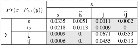
The results of estimating D ∈ SPD2 with
the corpus is shown in Table 6. The results clearly demonstrate the effectiveness of the model: the probability of a [α anterior] sibilant given P≤1([-αanterior])sounds is orders of magnitude less than givenP≤1(αanterior])sounds.
x P r(x|P≤1(y))
s >ts S >tS s 0.0335 0.0051 0.0011 0.0002 ⁀ts 0.0218 0.0113 0.0009 0.
y S 0.0009 0. 0.0671 0.0353
>
[image:9.595.306.532.418.491.2]tS 0.0006 0. 0.0455 0.0313
Table 1: Results of SP2 estimation on the Samala
corpus. Only sibilants are shown.
7 Conclusion
SP distributions are the stochastic version of SP languages, which model long-distance dependen-cies. Although SP distributions distinguish2|Σ|k−1 states, they do so with tractably many parameters and states because of an assumption that distinct subsequences do not interact. As shown, these distributions are efficiently estimable from posi-tive data. As previously mentioned, we anticipate these models to find wide application in NLP.
4The corpus was kindly provided by Dr. Richard
Apple-gate and drawn from his 2007 dictionary of Samala.
5Samala actually contrasts glottalized, aspirated, and
References
R.B. Applegate. 1972. Inese˜no Chumash Grammar. Ph.D. thesis, University of California, Berkeley.
R.B. Applegate. 2007. Samala-English dictionary : a
guide to the Samala language of the Inese˜no Chu-mash People. Santa Ynez Band of ChuChu-mash
Indi-ans.
Eric Bakovi´c. 2000. Harmony, Dominance and
Con-trol. Ph.D. thesis, Rutgers University.
D. Beauquier and Jean-Eric Pin. 1991. Languages and scanners. Theoretical Computer Science, 84:3–21.
Eric Brill. 1995. Transformation-based error-driven learning and natural language processing: A case study in part-of-speech tagging. Computational
Lin-guistics, 21(4):543–566.
J. A. Brzozowski and Imre Simon. 1973. Character-izations of locally testable events. Discrete
Mathe-matics, 4:243–271.
Noam Chomsky. 1956. Three models for the descrip-tion of language. IRE Transacdescrip-tions on Informadescrip-tion
Theory. IT-2.
J. S. Coleman and J. Pierrehumbert. 1997. Stochastic phonological grammars and acceptability. In
Com-putational Phonology, pages 49–56. Somerset, NJ:
Association for Computational Linguistics. Third Meeting of the ACL Special Interest Group in Com-putational Phonology.
Colin de la Higuera. in press. Grammatical
Infer-ence: Learning Automata and Grammars. Cam-bridge University Press.
Pedro Garc´ıa and Jos´e Ruiz. 1990. Inference ofk -testable languages in the strict sense and applica-tions to syntactic pattern recognition. IEEE
Trans-actions on Pattern Analysis and Machine Intelli-gence, 9:920–925.
Pedro Garc´ıa and Jos´e Ruiz. 1996. Learning k-piecewise testable languages from positive data. In Laurent Miclet and Colin de la Higuera, editors,
Grammatical Interference: Learning Syntax from Sentences, volume 1147 of Lecture Notes in Com-puter Science, pages 203–210. Springer.
Pedro Garcia, Enrique Vidal, and Jos´e Oncina. 1990. Learning locally testable languages in the strict sense. In Proceedings of the Workshop on
Algorith-mic Learning Theory, pages 325–338.
Gunnar Hansson. 2001. Theoretical and typological
issues in consonant harmony. Ph.D. thesis,
Univer-sity of California, Berkeley.
Bruce Hayes and Colin Wilson. 2008. A maximum en-tropy model of phonotactics and phonotactic learn-ing. Linguistic Inquiry, 39:379–440.
Jeffrey Heinz. 2007. The Inductive Learning of Phonotactic Patterns. Ph.D. thesis, University of
California, Los Angeles.
Jeffrey Heinz. to appear. Learning long distance phonotactics. Linguistic Inquiry.
John Hopcroft, Rajeev Motwani, and Jeffrey Ullman. 2001. Introduction to Automata Theory, Languages,
and Computation. Addison-Wesley.
Frederick Jelenik. 1997. Statistical Methods for Speech Recognition. MIT Press.
C. Douglas Johnson. 1972. Formal Aspects of
Phono-logical Description. The Hague: Mouton.
A. K. Joshi. 1985. Tree-adjoining grammars: How much context sensitivity is required to provide rea-sonable structural descriptions? In D. Dowty, L. Karttunen, and A. Zwicky, editors, Natural
Lan-guage Parsing, pages 206–250. Cambridge
Univer-sity Press.
Daniel Jurafsky and James Martin. 2008. Speech and Language Processing: An Introduction to Nat-ural Language Processing, Speech Recognition, and Computational Linguistics. Prentice-Hall, 2nd
edi-tion.
Ronald Kaplan and Martin Kay. 1994. Regular models of phonological rule systems. Computational
Lin-guistics, 20(3):331–378.
Gregory Kobele. 2006. Generating Copies: An
In-vestigation into Structural Identity in Language and Grammar. Ph.D. thesis, University of California,
Los Angeles.
Leonid (Aryeh) Kontorovich, Corinna Cortes, and Mehryar Mohri. 2008. Kernel methods for learn-ing languages. Theoretical Computer Science,
405(3):223 – 236. Algorithmic Learning Theory.
M. Lothaire, editor. 1997. Combinatorics on Words. Cambridge University Press, Cambridge, UK, New York.
A. A. Markov. 1913. An example of statistical study on the text of ‘eugene onegin’ illustrating the linking of events to a chain.
Robert McNaughton and Simon Papert. 1971.
Counter-Free Automata. MIT Press.
A. Newell, S. Langer, and M. Hickey. 1998. The rˆole of natural language processing in alternative and augmentative communication. Natural Language Engineering, 4(1):1–16.
Dominique Perrin and Jean-Eric Pin. 1986. First-Order logic and Star-Free sets. Journal of Computer
and System Sciences, 32:393–406.
Catherine Ringen. 1988. Vowel Harmony: Theoretical
James Rogers and Geoffrey Pullum. to appear. Aural pattern recognition experiments and the subregular hierarchy. Journal of Logic, Language and
Infor-mation.
James Rogers, Jeffrey Heinz, Matt Edlefsen, Dylan Leeman, Nathan Myers, Nathaniel Smith, Molly Visscher, and David Wellcome. to appear. On lan-guages piecewise testable in the strict sense. In
Pro-ceedings of the 11th Meeting of the Assocation for Mathematics of Language.
Sharon Rose and Rachel Walker. 2004. A typology of consonant agreement as correspondence. Language, 80(3):475–531.
Jacques Sakarovitch and Imre Simon. 1983. Sub-words. In M. Lothaire, editor, Combinatorics on
Words, volume 17 of Encyclopedia of Mathemat-ics and Its Applications, chapter 6, pages 105–134.
Addison-Wesley, Reading, Massachusetts.
Stuart Shieber. 1985. Evidence against the context-freeness of natural language. Linguistics and
Phi-losophy, 8:333–343.
Imre Simon. 1975. Piecewise testable events. In
Automata Theory and Formal Languages: 2nd Grammatical Inference conference, pages 214–222,
Berlin ; New York. Springer-Verlag.
Howard Straubing. 1994. Finite Automata, Formal
Logic and Circuit Complexity. Birkh¨auser.
Wolfgang Thomas. 1982. Classifying regular events in symbolic logic. Journal of Computer and Systems
Sciences, 25:360–376.
Enrique Vidal, Franck Thollard, Colin de la Higuera, Francisco Casacuberta, and Rafael C. Carrasco. 2005a. Probabilistic finite-state machines-part I.
IEEE Transactions on Pattern Analysis and Machine Intelligence, 27(7):1013–1025.
Enrique Vidal, Frank Thollard, Colin de la Higuera, Francisco Casacuberta, and Rafael C. Carrasco. 2005b. Probabilistic finite-state machines-part II.