Estimating empirical codon hidden Markov models

Nicola De Maio,*

,1

Ian Holmes,

2

Christian Schlo¨tterer,

1

and Carolin Kosiol

1 1_{Institut fu}

¨r Populationsgenetik, Vetmeduni Vienna, Wien, Austria

2_{Department of Bioengineering, University of California, Berkeley}

*Corresponding author:E-mail: [email protected]. Associate editor:Xun Gu

Abstract

Empirical codon models (ECMs) estimated from a large number of globular protein families outperformed mechanistic codon models in their description of the general process of protein evolution. Among other factors, ECMs implicitly model the influence of amino acid properties and multiple nucleotide substitutions (MNS). However, the estimation of ECMs requires large quantities of data, and until recently, only few suitable data sets were available. Here, we take advantage of several newDrosophilaspecies genomes to estimate codon models from genome-wide data. The availability of large numbers of genomes over varying phylogenetic depths in theDrosophilagenus allows us to explore various divergence levels. In consequence, we can use these data to determine the appropriate level of divergence for the estimation of ECMs, avoiding overestimation of MNS rates caused by saturation. To account for variation in evolutionary rates along the genome, we develop new empirical codon hidden Markov models (ecHMMs). These models significantly outperform previous ones with respect to maximum likelihood values, suggesting that they provide a better fit to the evolutionary process. Using ECMs and ecHMMs derived from genome-wide data sets, we devise new likelihood ratio tests (LRTs) of positive selection. We found classical LRTs very sensitive to the presence of MNSs, showing high false-positive rates, especially with small phylogenies. The new LRTs are more conservative than the classical ones, having acceptable false-positive rates and reduced power.

Key words:empirical codon model, rate heterogeneity, hidden Markov models, positive selection,Drosophilasubstitution patterns.

Introduction

Markov models of genomic sequence evolution are widely used in bioinformatics and usually belong to one of three classes: nucleotide, amino acid, or codon models. Nucleotide models are widely used, even for coding sequences (CDSs), because of their simplicity and broad applicability. Amino acid models are more often applied to diverged alignments. However, it has been shown that codon models should be preferred over both nucleotide and amino acid models when describing CDS evolution (Shapiro et al. 2006;Seo and Kishino 2009), unless the number of sequences in the alignment makes their use too computationally demanding.

Furthermore, codon models have the convenient property of being able to detect selective forces acting along protein-coding DNA sequences by distinguishing between nonsynonymous (amino acid replacing) and synonymous (silent) codon changes. They have therefore long been applied to detect positive selection (for reviews see Yang and Bielawski 2000;Anisimova and Liberles 2007).

Traditionally, codon models are defined as mechanistic and rely on a very small number of parameters (e.g., the model M0, Yang et al. 2000). However, empirical features have been introduced in codon models by Doron-Faigenboim and Pupko (2007), who proposed a combination of a mechanistic codon model (whose parameters are esti-mated per gene or small genomic region) with an empirical

amino acid model (which is instead pre-estimated from large databases and thus fixed). Later, other semiempirical models incorporating amino acid propensities were devised (e.g., Delport et al. 2010;Rodrigue et al. 2010).

With larger and more numerous genomic data sets and more powerful computers, models with increasing complex-ity have been proposed (for a review see Anisimova and Kosiol 2009). These new approaches account for phenomena such as selection acting on synonymous codon substitutions (see e.g.,Nielsen et al. 2007) and substitutions affecting more than one nucleotide (multiple nucleotide substitutions [MNSs], see e.g.,Whelan and Goldman [2004]).

Kosiol et al. (2007)estimated a full empirical codon model (ECM) by maximum likelihood. ECMs need large amounts of data to be estimated but implicitly account for many biologically relevant phenomena without making any as-sumptions except for reversibility of the Markov process. In particular, instantaneous double and triple nucleotide changes within one codon are accommodated by allowing for nonzero instantaneous MNS rates in the codon substitu-tion matrix. These changes may result from mutasubstitu-tional events that affect multiple nearby nucleotides (e.g., see Schrider et al. 2011). With the classical ECM, all possible MNSs between codons are treated individually. In this article, however, we propose a new simplified ECM that makes use of considerably fewer free parameters when incorporating MNSs.

Article

ßThe Author(s) 2012. Published by Oxford University Press on behalf of the Society for Molecular Biology and Evolution. This is an Open Access article distributed under the terms of the Creative Commons Attribution Non-Commercial License (http://creativecommons.org/licenses/by-nc/3.0/), which permits unrestricted non-commercial use, distribution, and reproduction

The classical ECM does not account for the heterogeneity of the evolutionary process along the genome. For example, some genes or some parts of genes might evolve at signifi-cantly slower rates than others due to stronger purifying se-lection or lower mutation rates. Thus, models assuming homogeneity of rates across a sequence might not be ad-equate. In fact, using such a rate-homogeneous model can create a bias, for example, by over-estimating the amount of MNSs (Smith et al. 2003). For nucleotide models, several approaches have been pursued to account for rate hetero-geneity among sites.Yang (1993)used a gamma distribution to model the pattern of substitution rates among sites.Yang (1995) and Felsenstein and Churchill (1996) used hidden Markov models (HMMs), which not only allow different sites to belong to different evolution classes but also describe cases in which neighboring sites tend to belong to the same class. Since then, the application of HMMs for the analysis of comparative genomic data has been very fruitful (reviewed in Siepel and Haussler 2004).

Among-site rate variation has also been incorporated into codon models. In particular, in addition to incorporating het-erogeneity in the total rate of substitutions (as in nucleotide models), heterogeneity in selection pressure is modeled via discrete and continuous distributions for the nonsynon-ymous/synonymous rate ratio (Yang et al. 2000). Heger et al. (2009) implemented a mechanistic codon model within the software package XRATE (Klosterman et al. 2006) with an HMM structure distinguishing the two selective regimes of intracellular and secreted regions of transmem-brane proteins. In general, XRATE allows the definition of an HMM along the sequence as a particular case of a “phylo-grammar” (Knudsen and Hein 1999), a tool commonly used to infer protein and gene structure.

In this study, we incorporate HMMs into ECMs. First, we estimate simple ECMs from new genomic data sets from several lineages and clades across theDrosophilaphylogeny. Then we use the framework of XRATE to create an empirical codon HMM (ecHMM): we extend ECMs with an HMM structure along the sequence defining different classes ac-counting for variation in codon usage and selective pressure on amino acids.

Although codon models have also been applied to phylo-genetic estimation (Ren et al. 2005) and classification of gen-omic sequences (seeLin et al. 2011, for an application of ECMs in this field), they are most commonly used to test for positive selection. We demonstrate the utility of our newly devised ECMs and ecHMMs by using them in tests of positive selec-tion on simulated data and on a real data set of 181 Drosophila immunity genes previously investigated by Sackton et al. (2007).

Materials and Methods

Basic Markov Models for CDSs

Most codon models in common use describe CDS evolution as a continuous time Markov process. The process is further assumed to be time homogeneous and thus can be defined by an instantaneous rate matrixQ¼ fqijg, whose elements

specify instantaneous rates of change among the 61 sense codons. Substitutions to/from stop codons are not allowed, because such events are usually not tolerated by a functional protein. The diagonal elements of Q are defined by the mathematical requirement that the rows sum up to zero (i.e.,qii¼

P

j6¼iqij). Given such aQ, the substitution

prob-ability matrix of the Markov process can be calculated as PðtÞ ¼ fpijðtÞg ¼eQt, where each entrypijðtÞis the

probabil-ity that codoniis substituted by codonjafter timet. In the ECM (see Kosiol et al. 2007), the instantaneous substitution rate from codonito codonj6¼iis defined as

qij¼sijj ð1Þ

wheresij¼sjiis called an exchangeability parameter, andjis

the frequency of codonj. Therefore, the number of free par-ameters in the ECM is 61

2

¼1,830 forfsijgand further 60 for

fjg, so 1,890 in total.

Because such a large number of free parameters is undesir-able, we tested whether the ECM could maintain a compar-able performance with greatly reduced complexity. Our new version of the ECM, the simplified ECM, is obtained by sum-marizing all exchangeability parameters modeling MNSs with four parameters. The new exchangeability parameters are ob-tained setting the following constraints:

qij ¼

sijj if i!j single nucleotide change

s2sj if i!j double syn:nt change

s2nsj if i!j double nonsyn:nt change

s3sj if i!j triple syn:nt change

s3nsj if i!j triple nonsyn: nt change, 8

> > > > < > > > > :

ð2Þ

thus the four parameterss2s,s2ns,s3s ands3ns replace 1,567

parameters of the ECM (eq. 1), reducing the total number of free parameters to 323. For small data sets, the estimation of s2sands3smight be based only on few MNSs (supplementary

table S2,Supplementary Materialonline) and thus will not be reliable (supplementary fig. S8, Supplementary Material online). Nevertheless, the estimation of these parameters is less prone to overfitting than the estimation of those in the classical ECM.

Supplementary files S1 and S2, Supplementary Material online, define, respectively, the ECM and the simplified ECM as phylo-grammars. They are the input files we used in XRATE to estimate the model parameters. We also devised other variants of the general ECM and investigated different levels of model complexity without presumptions about what might best fit real sequence data (see supplementary text, Supplementary Materialonline).

Empirical Codon Hidden Markov Models

codon to fall in one class also depends on the class of nearby codons (each codon is not independent of the others). In this model, evolutionary features can differ for each class, but the process is assumed to be homogeneous along the phylogeny. In particular, here we focus on modeling two variable aspects in sequence evolution: codon usage (with codon usage site classes or cu-classes) and nonsynonymous substitution rate (withR-classes, see later).

Given any two HMM site classes, C0 andC1, we define

the free parameter 01 as the probability that a codon

belongs toC1 conditioned on the previous codon belonging

toC0. Similarly,10 represents the probability that a codon

belongs toC0 conditioned on the previous codon

belong-ing toC1 (consequently 00¼101 and 11¼110).

For a more detailed description of the HMM parameter space, see thesupplementary text,Supplementary Material online.

Although some ecHMM parameters are defined for a single class, most of them are shared among classes. For ex-ample, to model variation in codon usage, we define a set of 60 free parametersfðkÞ_g

describing codon frequencies for each classk. In contrast, all the exchangeability parameters have the same values for allKclasses. The instantaneous rates for cu-classkare therefore:

qð_ijkÞ¼sij

ðkÞ

j ; ð3Þ

for anyk2 f0,1,. . .,K1g, whereKis the total number of classes. An ecHMM with K cu-classes will be called K cu-ecHMM (Kcodon usage classes ecHMM).

Alternatively, to model variation in the total nonsynon-ymous substitution rate, we use one parameterRin each class (R-class). Here RðkÞ (k2 f0,1,. . .,K1g) represents the relative nonsynonymous rate in classkwith respect to the first class (Rð0Þ_{¼1). R has a general discrete distribution} among classesf1, . . .,K1g. The instantaneous rates for R-classkare:

qð_ijkÞ¼ sijj if i!jsyn:change

RðkÞsijj if i!jnonsyn: change:

ð4Þ

The nonsynonymous rate for the first class (k¼0) is only determined by the exchangeabilitiesfsijg. Also, the

exchange-ability values are shared among all the classes. The only dif-ference betweenR and the parameter! of classical codon models is that hereR¼1 does not need to correspond to neutrality. We call this model withKclassesKR-ecHMM.

In all ecHMMs, the fsijgare as defined in the simplified

ECM (eq. 2). The fsijg parameter values are always shared

among classes and are estimated together with the class-specific parameters,RðkÞ_orfðkÞ_{g. More ecHMMs can} be obtained defining cu-classes (eq. 3) andR-classes (eq. 4) within a single model. For example, we combine two R-classes and two cu-classes into a 2R-2cu-ecHMM. This model is pre-sented as input phylo-grammar for the software XRATE in supplementary file S3, Supplementary Materialonline. This and further types of ecHMM are presented and discussed in thesupplementary text,Supplementary Materialonline.

Models for Positive Selection Tests

The classical Goldman–Yang model M0 (Goldman and Yang 1994;Yang et al. 2000) is defined as

qij¼

j i!j syn: transversion j i!j syn: transition !j i!j nonsyn:transversion !j i!j nonsyn:transition

0 i!j MNS; 8

> > > > < > > > > :

ð5Þ

whereis the transition/transversion rate ratio, and!is the nonsynonymous/synonymous rate ratio.

Here, we modify this model to include the genome-wide empirical codon exchangeability parameter estimates^sij. This

way, the number of free parameters remains unchanged, but the new model accounts for MNSs and for different instan-taneous substitution rates among codons:

qij¼

^

sijj i!jsyn:transversion

^

sijj i!jsyn:transition

^

sij!j i!jnonsyn:transversion

^

sij!j i!jnonsyn:transition

^

sijj i!jsyn:MNS

^

sij!j i!jnonsyn:MNS: 8

> > > > > > < > > > > > > :

ð6Þ

Here, the ^sij are constants, whereas !, , and j are free

parameters. We call this model ecM0. Note that despite including empirical estimates, this model has only a small number of free parameters. Therefore, this model is appro-priate for data sets as small as a single gene.

ECM exchangeability parameters (^sij in eq. 6) implicitly

include information about the genome-wide average transi-tion/transversion rate^and the genome-wide average non-synonymous/synonymous rate!^. Therefore, values ofand

!in ecM0 (eq. 6) do not have necessarily the same interpre-tation as in M0 (eq. 5).

We do not correct for the difference in estimates, because we are not interested in interpreting or comparing them. In contrast, in eq. 6, we want to associate purifying selection to values of!below a certain threshold and positive selection to values above it. A natural choice for this threshold is 1=!^, once we have precisely defined!^.

As an estimate of!^,Kosiol et al. (2007)used

!E¼

a

_s

0:21

0:79; ð7Þ

wherea¼Pði,jÞ2N ^iq^ijis the total substitution rate of the

set of nonsynonymous codon pairs N. Similarly _s¼

P

ði,jÞ2S^iq^ijis the total substitution rate over the set of

syn-onymous codon pairsS. The constant 0:79=0:21 associated with neutrality was determined byNei and Gojobori (1986). This method is not robust to variation in the transition/ transversion rate ratio. For example, if we consider the model M0 (eq. 5) as an ECM estimate, we would like!Eto

approx-imate!. However, keeping!constant in M0 and varying, the estimate !E changes (supplementary table S1,

transversions, or equivalently most transitions are synon-ymous. Increasingtherefore increasessrelative toa.

An appropriate definition of !^ is fundamental for the identification of positive selection. Therefore, we pursue a different, more robust, strategy, aimed at having an!^ that gives values comparable to the!of M0. The idea is to esti-mate nonsynonymous/synonymous rate ratios for transitions and transversions separately and then average them. More specifically, we estimate a distinct nonsynonymous/synon-ymous rate ratio for each mutation typen1!n2, withn1

the ancestral nucleotide andn2 the derived nucleotide.

First, we define the average nonsynonymous rate for muta-tionn1 !n2

qNn1!n2 ¼

P

ði,jÞ 2 Nn1!n2

^

iq^ij

P

ði,jÞ 2 Nn1!n2

^

i

; ð8Þ

and the average synonymous rate for mutationn1 !n2

qSn1!n2 ¼

P

ði,jÞ 2 Sn1!n2

^

iq^ij

P

ði,jÞ 2 Sn1!n2

^

i

: ð9Þ

HereNn1,n2 (Sn1,n2) is the set of nonsynonymous

(synon-ymous) codon pairsði,jÞcorresponding to substitutions from codonitojthat involve a single mutationðn1!n2Þ.

The nonsynonymous/synonymous rate ratio forn1 !n2

is then

^

!n1!n2¼

qN_n

1!n2

qSn1!n2

, ð10Þ

and the final !^ is obtained by averaging !^n1!n2 over all

mutations:

^

!¼

P n1!n2

^

!n1!n2

P

ði,jÞ 2 fNn1!n2[Sn1!n2g

^

i

P n1!n2

P

ði,jÞ 2 fNn1!n2[Sn1!n2g

^

i

: ð11Þ

If we consider the model M0 as a special case of an ECM, we observe that!^ recovers!correctly, independently of( sup-plementary table S1,Supplementary Materialonline). To keep the notation simple, we multiply all nonsynonymous f^sijg

(eq. 6) by the factor 1=!^, so that!¼1 in the ecM0 will correspond to neutrality as in M0.

After this modification, Model ecM0 can be used to estimate the average selective pressure on amino acids within a gene. However, to infer positive selection limited to only a few sites of a gene, we need a model allowing for different!at different sites. Among-site variation of!can be described by any of several probability distributions. The simplest site models use the general discrete distribution with a prespecified number of site classesK. Each site class i¼0,1;. . .,K1 has a specific ratio parameter!i and a

specific proportionpiof sites belonging to it. The discretized

versions of continuous distributions (such as gamma and beta) or mixture distributions have been also successfully applied to positive selection scans (Yang et al. 2000).

Here, we modify the most popular models to include empirical parameter estimates (as we did for ecM0 in eq. 6). Analogous to M1a (Yang et al. 2005), we define ecM1a as a model with two site classes, one for purifying selection (!0<1) and the other for neutrality (!1¼1).

This model lacks sites with ! >1 and, therefore, can be used as a null hypothesis in tests of positive selection. Analogous to the alternative model of M1a, M2a (Yang et al. 2005), the alternative model ecM2a extends ecM1a by adding a further (third) site class with!2>1 to

accommo-date sites evolving under positive selection.

Similarly, we modify another test comparing the model M7 versus M8 (Yang et al. 2000). The model ecM7 has a beta-distributed!(with 0< ! <1), whereas ecM8 has a discrete class for positive selection (! >1) and a beta-distributed!

(with 0< ! <1) in the rest of the codons. We approximate the beta distribution with 10 site classes. Significance of the likelihood ratio tests (LRT) was determined at the 5%and 1%level with a2

2distribution. A summary of these models

is given intable 1.

We will provide our modified version of codeml (from PAML 4.2) that we used for tests of positive selection with empirical models upon request.

Genomic Data Sets

We trained our models on codon alignments of a subset of the 12Drosophilagenomes (Stark et al. 2007) consisting of D. melanogaster (Dmel), D. simulans (Dsim), D. yakuba (Dyak), andD. ananassae(Dana). The choice of species was made to minimize incomplete lineage sorting (see Pollard et al. 2006) and saturation caused by large divergence. For some of the analyses, we added a second Dmel sequence derived from the consensus of 5 full-genome sequenced indi-viduals from the Raleigh population of the 50 Drosophila genomes project (Release 1.0, http://www.dpgp.org/; last accessed 7 Dec 2012).

Whole-genome CDS alignments were downloaded from the UCSC table browser (http://genome.ucsc.edu/; last accessed 7 Dec 2012). We included only one alignment for each Dmel CDS and excluded CDS alignments with more than 25% of divergence between any two species. We excluded CDS alignments with nonsense codons or frame shifts. We also trimmed start and stop codons (stop codons could thereby be excluded from the models). Number of codons and number of CDSs for each data set are listed intable 2.

in the supplementary text, Supplementary Material online. The same protocol was used for the species pair Dpse– Dlow by Palmieri et al. (personal communication) who kindly gave us access to the alignments.

Finally, we performed a positive selection scan on a real data set of 181 immune system genes that was created by Sackton et al. (2007). Orthologous gene alignments were kindly provided to us by the author. These alignments

comprise six species:Dmel, Dsim, D. sechellia (Dsec), Dyak, D. erecta(Dere),andDana.

Simulations

CDS alignments were simulated using the program SimGram (Varadarajan et al. 2008) in the DART package.

To test the accuracy of the estimation procedure, we simu-lated data sets using three different ECM real data estimates (from the two, three, and four speciesmelanogasterdata sets), three different phylogenetic trees estimated from real data (again the two, three, and four species melanogaster data sets), and seven different total alignment lengths (5104, 105, 2105, 5105, 106, 2106, and 3106 codons). We then estimated ECMs from these simulated data sets and checked how well they recovered the true ECMs.

We also tested the accuracy of the estimation of the 2cu-ecHMM (a Kcu-ecHMM with K¼2). We simulated data according to the 2cu-ecHMM estimated onDmel–Dsimand according to the tree from the same data. Although single exons where simulated with the same mean length as in real data, the total alignment length was 104_{, 210}4_{, 510}4_{, 10}5_,

2105_{, 510}5_{, or 10}6_codons.

We created a third set of simulated data to compare the performance of mechanistic and empirical tests of positive selection. Each scenario consists of 1,000 genes, each 500 codons long. The simulations were performed on three dif-ferent phylogenetic trees (the ones estimated onDmel–Dsim, on Dmel–Dsim–Dyak, and on Dmel–Dsim–Dsec–Dyak– Dere–Dana). However, we always simulated under the 2cu-ecHMM substitution model estimated from theDmel–Dsim alignments (but using only one of the two estimated sets of codon frequencies). The four scenarios we chose to study the statistical behavior of our tests were inspired byWong et al. (2004): we have two scenarios with positive selection and two without (see supplementary table S10, Supplementary Material online, for detailed description of the parameter choices). Corresponding selective pressures are obtained by scaling the nonsynonymous substitution rates in the empiri-cal model, so that a neutral codon is simulated according to an ECM with !^ ¼1. Choosing these scenarios made our results comparable to those ofWong et al. (2004), although those were obtained simulating under classical mechanistic codon models, that is, without MNSs.

The last simulated data set was created to test the perfor-mance of ecHMMs in detection of positive selection. In con-trast to the other simulations, the codon sites were simulated nonindependently, such that each codon position had a high probability (50%) of having the same selective pressure than the previous one (see supplementary table S10, Supplementary Materialonline, for details). Again we simu-lated 1,000 genes, each of 500 codons, for each of four scenar-ios, two with positive selection and two without. We use a tree with eight species and with uniform branch lengths. Furthermore, we use the ECM estimated onDmel–Dsim– Dyakto simulate substitutions.

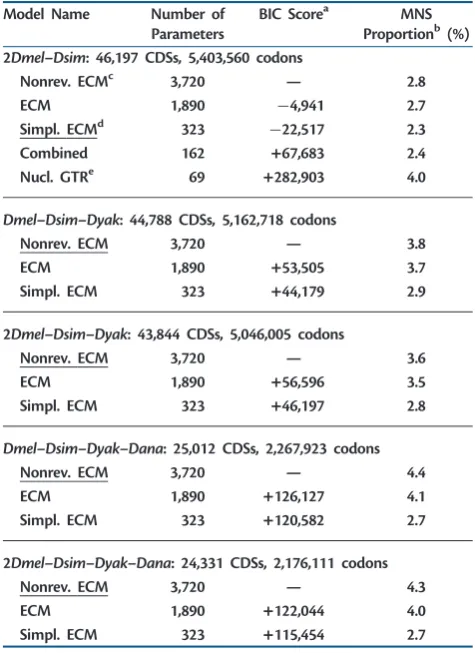
[image:5.595.50.287.63.145.2]

All details for all simulation scenarios are summarized in supplementary table S10,Supplementary Materialonline. Table 2. Performances of Models with Different Levels of Complexity

on Real Data

Model Name Number of

Parameters

BIC Scorea MNS

Proportionb(%) 2Dmel–Dsim: 46,197 CDSs, 5,403,560 codons

Nonrev. ECMc 3,720 — 2.8

ECM 1,890 4,941 2.7

Simpl. ECMd 323 22,517 2.3

Combined 162 +67,683 2.4

Nucl. GTRe 69 +282,903 4.0

Dmel–Dsim–Dyak: 44,788 CDSs, 5,162,718 codons

Nonrev. ECM 3,720 — 3.8

ECM 1,890 +53,505 3.7

Simpl. ECM 323 +44,179 2.9

2Dmel–Dsim–Dyak: 43,844 CDSs, 5,046,005 codons

Nonrev. ECM 3,720 — 3.6

ECM 1,890 +56,596 3.5

Simpl. ECM 323 +46,197 2.8

Dmel–Dsim–Dyak–Dana: 25,012 CDSs, 2,267,923 codons

Nonrev. ECM 3,720 — 4.4

ECM 1,890 +126,127 4.1

Simpl. ECM 323 +120,582 2.7

2Dmel–Dsim–Dyak–Dana: 24,331 CDSs, 2,176,111 codons

Nonrev. ECM 3,720 — 4.3

ECM 1,890 +122,044 4.0

Simpl. ECM 323 +115,454 2.7

NOTE.—The best model for each data set according to BIC score is underlined.

a

BIC score difference between the current model and the nonreversible ECM trained on the same data set (models with smaller BIC score are considered preferable).

b_{Estimated proportion of MNSs.} c_{Nonreversible empirical codon model.} d_{Simplified empirical codon model.} e

[image:5.595.49.287.217.544.2]

Codon extension of the nucleotide general time reversible model.

Table 1. Models Used for Tests of Positive Selection

Model Parametersa _{Number of}

Free Parameters M1a, ecM1a p0, (p1¼1p0),!0<1,!1¼1 2 M2a, ecM2a p0,p1, (p2¼1p0p1),

!0<1,!1¼1,!2>1

4

M7, ecM7 p,q 2

M8, ecM8 p0, (p1¼1p0),p,q,!1>1 4

a_{Parameters describing selective pressure distribution:!irefers to selective pressure}

in classi (!¼1 corresponding to neutrality), andpi is the proportion of sites

Tree Estimation

For the estimation of empirical models with Xrate, and for simulations with SimGram, we used phylogenetic trees that were estimated on whole-genome data sets using baseml (Yang 2007) with model HKY85+. Whenever simulated data were used, the correct tree was fixed for the estimation of the models, except in positive selection tests with codeml (Yang 2007), where branch lengths were re-estimated with codeml itself.

Results and Discussion

Simplified ECM

We estimated codon models with various levels of complexity to compare model performances and estimates of MNSs. In particular, we were interested in investigating whether the complexity of the ECM could be reduced without affecting its performance. To this end, models were fitted on data sets spanning different levels of species divergence. When only Dmel and Dsim were aligned, their divergence (calculated here as the proportion of mismatching bases) was 4:0%. WhenDyakis also included, the divergence betweenDmel andDsimis reduced because many poorly conserved CDSs are lost from the data set, and the divergence betweenDmel and the outgroup (Dyak) becomes 7:7%. Similarly, when Danais added, the divergence betweenDmeland the out-groupDanais 15:8%. Performances of codon models were compared with AIC (Akaike 1974) and BIC (Schwarz 1978) scores.

Generally, we find that more complex models tend to fit the data better, and this is even more pronounced if using AIC instead of BIC (table 2 and supplementary table S3, Supplementary Materialonline). The empirical models out-performed the codon extension of the nucleotide general time reversible (GTR) model (see supplementary text, Supplementary Material online), as expected, because the latter model cannot account for amino acid affinities. Our Combined model (obtained by combining an empirical amino acid and a nucleotide GTR model into a codon model, see supplementary text, Supplementary Material online) was also outperformed by ECMs, although it contains empirical amino acid affinities and mutation rate parameters. As both the nucleotide GTR and the Combined models were strongly and generally outperformed (supplementary table S3, Supplementary Material online), both were removed from further analysis.

Interestingly, the simplified ECM was always preferred by BIC score to the standard ECM (but not by AIC score,table 2). The nonreversible ECM (seesupplementary text, Supplemen-tary Materialonline) only performed better than the reversi-ble ECMs when more diverged species such asDyakandDana were added to the closely related species pairDmel–Dsim. The reason might be that in theDmel–Dsimdata set, there are fewer substitutions, and this favors simpler models.

We investigated the accuracy of our methods in estimating ECMs and recovering evolutionary features. For this purpose, we used data sets simulated according to three different phylogenetic trees and three different ECMs (see Materials

and Methods). We then estimated an ECM and a simplified ECM on each data set and compared the estimated para-meters with the true ones used for simulations. As a measure of the estimation error, we used the Euclidean distance between the vector of parameter estimates, and the vector of true parameters, normalized by the norm of the vector with true parameters. As expected, with increased alignment length, the estimation improved (fig. 1 and supplementary figs. S2 and S3, Supplementary Material online). On data simulated according to a short-branched phylogenetic tree, and according to genomic sizes (2,000,000 codons or more), the model parameters were recovered with error rate below 5%(fig. 1andsupplementary figs. S2andS3,Supplementary Materialonline).

For the largest tree (Dmel,Dsim, Dyak,and Dana), the estimates were unsatisfactory. This suggests that ECMs esti-mated on high-divergence data sets should not be used for interpreting evolutionary patterns, although they could still be used to describe sequence evolution because of their better fit to data in terms of BIC and AIC scores. Increasing the amount of data to beyond 106 codons had generally negligible effects on the accuracy of the estimates.

We also determined the proportion of MNSs in estimated ECMs, defined as:

MNS

¼

P

ði,jÞ 2 M ^

iq^ij

P

ði,jÞ ^

iq^ij

, ð12Þ

whereMis the set of pairs of codons separated by at least two nucleotide changes.

We estimated between 2:3%and 4:4%of MNSs in real data (table 2). The simplified ECM always showed lower pro-portions of MNS than the standard ECM. We interpret this as a symptom of overfitting for the standard model (see later). It is also noteworthy that for lower divergences (e.g.,Dmeland Dsim), estimates of MNS rates were smaller than for higher divergences (e.g.,Dmel,Dsim,Dyak,andDana).

In simulated data sets with low and medium divergence levels, estimates of MNS rate were relatively precise, in fact the difference between true and estimated proportion of MNSs was below 1%(fig. 2). For the most diverged simulated data set, large MNSs rates (far above the simulated ones) were estimated, suggesting that saturation and overfitting have contributed to MNS rate overestimation in this and in pre-vious studies with ECMs (e.g.,Kosiol et al. 2007). Other causes leading to MNS rate overestimation in real data are site and branch evolutionary heterogeneity. In fact, we later show that accounting for variability of evolutionary rates among sites reduces MNSs estimates.

Schrider et al. has to be considered an upper bound for our MNS rate. First, they analyzed both coding and non-CDSs, and in CDSs, MNMs are likely to be deleterious and, therefore, to be purged by selection. Second, Schrider et al. considered mutations separated by less than 20 bp to be MNMs, whereas we only considered changes within the same codon as MNSs. Third, we estimated the proportion of MNS events and not the proportion of nucleotides modified by MNSs, so that our estimates should be less than half of the 3%estimated by Schrider et al.

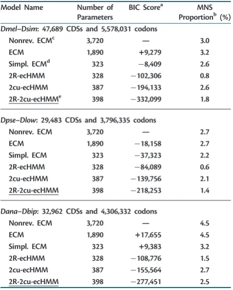
ECMs Estimated on Different

Drosophila

Clades

We repeated the analysis of the previous section on a larger collection of data sets to compare evolution among different clades of the genusDrosophilaand to seek confirmation of our previous results. As described in Materials and Methods section, we obtained sets of alignments for two additional pairs ofDrosophila species. The first alignment is between DanaandDbip(from theananassaeclade) and the second betweenDpseandDlow(from thepseudobscuraclade). The melanogasterclade is represented by theDmel–Dsim align-ment. From the observations of the previous section, we deduced that we could reliably estimate ECMs from these three pairwise alignments. We therefore used these three data sets to estimate all previously introduced ECMs. The compar-ison of different models led to the same ranking and con-firmed all other observations of the previous section (table 3 andsupplementary table S4,Supplementary Materialonline).

Here, we focus on the comparison between clades. We wanted to assess differences in CDS evolution among the clades and whether the difference scales with their phyloge-netic relatedness. It is a concern of this analysis that results can be biased by the different levels of divergence between species within the pairs. Although the divergenceDmel–Dsim is comparable to that ofDpse–Dlow(in the first alignment 4.01% of the bases are substituted, in the second 3.58%), Dana–Dbipshows much larger divergence (8.62%). In more divergent alignments, we found smaller estimates of the non-synonymous/synonymous rate ratio (!^ ’0:14 in Dmel– Dsim, !^ ’0:15 in Dpse–Dlow, and !^ ’0:07 in Dana– Dbip), probably due to the fact that with higher divergence we can only align more conserved genes. We also cannot exclude that other effects may act on the most diverged pair, such as higher saturation, which could make the para-meters estimates different from those from the other data sets.

However, despite all these possible biases, we found that CDS evolution is more similar between themelanogasterand ananassaeclades than it is for both compared to the pseu-dobscuraclade (table 4andsupplementary table S5, Supple-mentary Materialonline). This is consistent with the fact that melanogaster and ananassae are more phylogenetically related to each other than they are to pseudobscura. This result held when we compared instantaneous rates qij,

exchangeability parameters sij, or codon frequencies i

(table 4 and supplementary table S5, Supplementary 0 500000 1000000 1500000 2000000 2500000 3000000

2345678

NUMBER OF CODONS

% MNS

FIG. 2. Estimation of MNS rate with the ECM. Proportion of MNSs estimated with ECM using data simulated according to three real phy-logenetic trees: Dmel–Dsim (4), Dmel–Dsim–Dyak (), and Dmel– Dsim–Dyak–Dana (). Simulations are repeated according to three different ECMs: the one estimated onDmel–Dsim(red), the one on

Dmel–Dsim–Dyak (green), and the one onDmel–Dsim–Dyak–Dana

(blue). Values shown represent the percentage of all substitutions, which are MNSs. The horizontal lines show the correct values, that is, the percentage of MNSs that was present in the respective ECM used for simulations.

0 500000 1000000 1500000 2000000 2500000 3000000

0

5

10

15

20

25

30

NUMBER OF CODONS

% ERROR

FIG. 1. Estimation error of the ECM. Percent error in estimating ECM exchangeability parameters4and instantaneous substitution rates

with phylogenies consisting of: Dmel–Dsim (red),Dmel–Dsim–Dyak

(green), andDmel–Dsim–Dyak–Dana(blue). The ECM used for simula-tions is the one estimated on theDmel–Dsim–Dyak–Danadata set. The vertical purple line represents the amount of codons in the smallest real data set used. Similar results are observed when simulating according to different ECMs (supplementary figs. S2andS3,Supplementary Material

Materialonline).Supplementary figures S4–S6, Supplemen-tary Material online, show bubbleplot visualizations of the ECMs on the three different clades.

A cross validation experiment also indicated that the mel-anogasterandpseudobscuraclades have evolved differently.

We split both data sets into two subsets: one containing 99% of the CDSs (randomly chosen), used to train ECM substitu-tion matrices, and the remaining 1%of CDSs, used to assess the goodness of fit of the models. The best performing model was the one trained on the same clade it was tested on (see supplementary text,Supplementary Materialonline).

Empirical Codon Hidden Markov Models

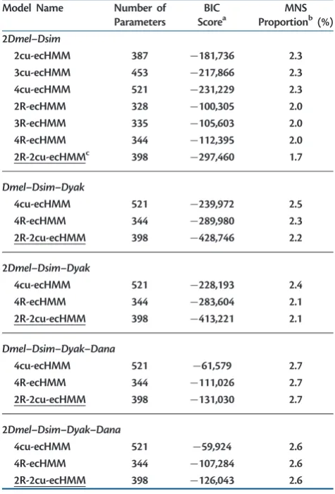
We estimated ecHMMs (see Materials and Methods) on the same data sets used previously for ECMs. In particular, we assessed whether empirical models that include site hetero-geneity better describe the process of sequence evolution and which heterogeneity feature leads to the largest improve-ment. Models with HMM structure usually outperform models with multiple independent classes or models in which codon classes are constant along exons (see supple-mentary text and supplementary tables S6 and S7, Supplementary Materialonline).

Using ecHMMs that account for variation in selective pres-sure (R-ecHMM, eq. 4), as well as ecHMMs modeling variation in codon usage (cu-ecHMM, eq. 3), always resulted in a sig-nificant increase of fit with respect to ECMs (tables 3and5 andsupplementary table S4,Supplementary Materialonline). However, using more than two site classes of the same type only brought a small fit increase (supplementary table S8, Supplementary Material online). The combination of the two class types in the same model (the 2R-2cu-ecHMM, see supplementary text,Supplementary Materialonline) always gave the best fit to data. Furthermore, R-ecHMM and cu-ecHMM were preferable to the modeling of variable transi-tion/transversion rate (-ecHMM), MNS rate (MNS-ecHMM), or total substitution rate (T-ecHMM) ( supplemen-tary table S7, Supplementary Material online). We also observed a general decrease in the estimated rate of MNSs in ecHMMs with respect to simple ECMs (table 5and sup-plementary table S8, Supplementary Material online), simi-larly to what shown bySmith et al. (2003)regarding MNMs. We tested whether an ecHMM can recover parameters from data with acceptable error and better precision than simple ECMs. We simulated alignments of different length under the 2cu-ecHMM (see Materials and Methods). On these, we estimated three models: the cu-ecHMM, the ECM, and the simplified ECM. The 2cu-ecHMM correctly recovered the codon frequencies of both classes (fig. 3). It also slightly improved the estimation of exchangeability rates (supplementary fig. S7, Supplementary Material online) and MNS rates with respect to simple ECMs (fig. 4). We also show the error in estimating each MNS parameter of the simplified ECM individually (supplementary fig. S8, Supplementary Materialonline).

[image:8.595.50.288.73.369.2]

In contrast, when simulating and estimating under the 2R-ecHMM, we did not recover the correct parameter values. The problem is likely a partially flat likelihood surface (see supplementary text, Supplementary Material online). This means that although the R-ecHMM and 2R-2cu-ecHMM might be often preferable in likelihood, their parameter esti-mates (in particular nonsynonymous rates) should not be Table 4. Comparisons between Models Estimated on Different

Clades

Featurea Dmel–Dsimvs.

Dana–Dbip (%)

Dmel–Dsimvs. Dpse–Dlow(%)

Dana–Dbipvs. Dpse–Dlow(%)

ECM Q 17.3 20.3 23.8

Simpl. ECM Q 16.8 20.3 23.1

2R-2cu-ecHMM Q 15.2 17.8 22.1

ECMp 7.0 12.5 12.7

ECM nucleotide 7.3 11.5 15.4

NOTE.—Comparison of parameter vectors estimated on different clades. Values show

the Euclidean distances between vectors, normalized by the average of the norm of the two vectors compared and expressed as a percentage.

a_{Model feature that is compared between clades: “Q” is the instantaneous}

[image:8.595.50.287.505.588.2]

substitu-tion rates matrix, “” is the codon frequencies vector, and “Nucleotide” stands for the nucleotide instantaneous substitution rates matrix extracted from the ECM averaging the single-nucleotide synonymous substitution rates for each ordered pair of nucleotides.

Table 3. Performance of ECMs Estimated on Data from Different

DrosophilaClades

Model Name Number of

Parameters

BIC Scorea MNS

Proportionb(%) Dmel–Dsim: 47,689 CDSs and 5,578,031 codons

Nonrev. ECMc 3,720 — 3.0

ECM 1,890 +9,279 3.2

Simpl. ECMd 323 8,409 2.6

2R-ecHMM 328 102,306 0.8

2cu-ecHMM 387 194,133 2.6

2R-2cu-ecHMMe _{398 332,099 1.8}

Dpse–Dlow: 29,483 CDSs and 3,796,335 codons

Nonrev. ECM 3,720 — 2.7

ECM 1,890 18,158 2.7

Simpl. ECM 323 37,323 2.2

2R-ecHMM 328 84,089 0.6

2cu-ecHMM 387 139,756 2.1

2R-2cu-ecHMM 398 218,253 1.4

Dana–Dbip: 32,962 CDSs and 4,306,332 codons

Nonrev. ECM 3,720 — 4.5

ECM 1,890 +17,655 4.5

Simpl. ECM 323 +9,383 3.2

2R-ecHMM 328 108,776 1.5

2cu-ecHMM 387 155,564 2.7

2R-2cu-ecHMM 398 277,451 2.5

NOTE.—The best model for each data set according to BIC score is underlined. a_{BIC score difference between the current model and the non reversible ECM}

trained on the same data set.

b

Proportion of MNSs estimated by the model.

c

Nonreversible empirical codon model.

d_{Simplified empirical codon model.}

e_{The ecHMM having two classes for nonsynonymous/synonymous rate ratio}

considered reliable. Therefore, we recommend the use of the cu-ecHMM instead.

The computational time required for the estimation of a 2cu-ecHMM from 106_{codons with a 2.66 GHz processor on a}

MacPro5.1 was6 h (seesupplementary table S9, Supple-mentary Materialonline, for more computational times of this and other ECMs).

Application of ECMs and ecHMMs to Tests of

Positive Selection

We assessed the performance with respect to the power and the amount of false positives for the new LRTs of positive selection. ecM1a–ecM2a (empirical with discrete!classes) and ecM7–ecM8 (empirical with beta-distributed!) were compared, respectively, to the classical tests M1a–M2a (mechanistic with discrete classes) and M7–M8 (mechanistic with beta-distributed!), on 1,000 genes simulated according to the same ECM used to define ecM0 (see Materials and Methods). Model estimations were here performed with a

modification of codeml, which is part of the PAML package (version 4.2).

[image:9.595.49.287.64.414.2]

We used some of the scenarios simulated byWong et al. (2004)that showed that the standard tests for positive selec-tion are conservative. However, for standard tests M1a–M2a Table 5. Performances of ecHMMs on Real Data

Model Name Number of

Parameters

BIC Scorea

MNS Proportionb(%) 2Dmel–Dsim

2cu-ecHMM 387 181,736 2.3

3cu-ecHMM 453 217,866 2.3

4cu-ecHMM 521 231,229 2.3

2R-ecHMM 328 100,305 2.0

3R-ecHMM 335 105,603 2.0

4R-ecHMM 344 112,395 2.0

2R-2cu-ecHMMc 398 297,460 1.7

Dmel–Dsim–Dyak

4cu-ecHMM 521 239,972 2.5

4R-ecHMM 344 289,980 2.3

2R-2cu-ecHMM 398 428,746 2.2

2Dmel–Dsim–Dyak

4cu-ecHMM 521 228,193 2.4

4R-ecHMM 344 283,604 2.1

2R-2cu-ecHMM 398 413,221 2.1

Dmel–Dsim–Dyak–Dana

4cu-ecHMM 521 61,579 2.7

4R-ecHMM 344 111,026 2.7

2R-2cu-ecHMM 398 131,030 2.7

2Dmel–Dsim–Dyak–Dana

4cu-ecHMM 521 59,924 2.6

4R-ecHMM 344 107,284 2.6

2R-2cu-ecHMM 398 126,043 2.6

NOTE.—The best model for each data set according to BIC score is underlined.

a

BIC score difference between the current model and the simplified ECM trained on the same data set.

b_{Proportion of MNSs estimated by the model.}

c_{The ecHMM having two classes for nonsynonymous/synonymous rate ratio}

varia-tion and two classes for codon usage variavaria-tion.

0e+00 2e+05 4e+05 6e+05 8e+05 1e+06

012345

NUMBER OF CODONS

% MNS

FIG. 4. Estimation of MNS rate with 2cu-ecHMM. Estimation of MNS rate on a data set simulated according to a 2cu-ecHMM model. On the

yaxis is proportion of substitutions that are MNSs, expressed in per-centage. On thexaxis is the number of codons in the respective data set used. Blue4represents the MNS rate estimated by a 2cu-ecHMM (the simulated model), redthe MNS rate estimated by a simplified ECM, and greenby an ECM. The horizontal line shows the simulated pro-portion of MNSs, that is, the true value to be estimated.

0e+00 2e+05 4e+05 6e+05 8e+05 1e+06

0

5

10

15

NUMBER OF CODONS

% ERROR IN CODON FREQ.

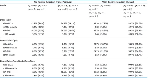
and M7–M8, we observed high proportions of false positives (table 6), often above acceptable levels, especially with small phylogenetic ftrees (e.g., 26.9%and 28.0% for theDmel– Dsimtree). In contrast toWong et al. (2004), we simulated with an ECM and therefore generated MNSs. These MNSs are not accounted for by classical models such as M1a–M2a or M7–M8 and will be interpreted as multiple substitutions clustered within the same codon and same branch. If these substitutions are nonsynonymous, they represent a signal of positive selection, especially with a small number of species.

For the analysis based on empirical models ecM1a–ecM2a and ecM7–ecM8, we found that the new tests are more conservative than the standard ones, having both acceptable false positives and reduced power (table 6). Alternatively, the problem of high false positives in classical tests could be solved by requiring a more stringent significance level, but this approach lowers the power of classical tests ( supplemen-tary table S13, Supplementary Material online) and priorly requires an extensive simulation study to determine an appropriate significance cutoff.

We addressed the question whether the different perfor-mance of the new tests was due to the generally more precise modeling of all substitutions or in particular to the inclusion of MNSs. For this reason, we used a modification of the new empirical models in which we set the rates of all multiple nucleotide changes to 0 (we call these new tests restricted). We also modified the classical M1a–M2a and M7–M8 to include MNSs (we call these variants +MNS models). We observed a drop in the false positives for the mechanistic +MNS models to a level comparable of the empirical

models (supplementary table S11, Supplementary Material online). Similarly, the restricted empirical tests showed high false positives. These two observations suggest that the dif-ference in performance is mainly attributable to the introduc-tion of MNSs in the model.

We also applied the new empirical tests to the real data set consisting of theDrosophilaimmune system gene alignments created bySackton et al. (2007)(see Materials and Methods). We included the ECM parameter estimates from Dmel– Dsim–Dyak–Danain the models ecM1a, ecM2a, ecM7, and ecM8, as constants. Most of the positives found with ecM7– ecM8 were also detected by M7–M8 (10 of 12), but never-theless the reduction in number of positives is remarkable: from 29 to 12 (supplementary fig. S9,Supplementary Material online). The test ecM1a–ecM2a found no positive genes.

Finally, we assessed whether the introduction of HMM structure could improve the detection of within-gene positive selection. In principle, this could happen if sites with positive selection tend to cluster (hypothesis confirmed inDrosophila byRidout et al. [2010]). Therefore, we modified the models ecM1a and ecM2a to include an HMM structure among the

! classes, the new models being called ecHMM1a and ecHMM2a (see supplementary text, Supplementary Materialonline). The tests were performed using Xrate and generally gave more conservative results than the previous tests performed with PAML. We simulated genes distributing

[image:10.595.50.547.63.324.2]

! according to an underlying HMM, clustering sites that shared similar selective constraints (see Materials and Methods and supplementary table S10, Supplementary Material online). In this context, the new LRTs seemed to Table 6. Performance of Positive Selection Tests on Simulated Data

No Positive Selection (False Positives) With Positive Selection (Power)

Model p0¼0:9, p1¼0:1 p0¼0:5, p1¼0:5 p0¼0:45, p1¼0:45, p0¼0:45, p1¼0:45,

x0¼0, x1¼1 x0¼0:5, x1¼1 p2¼0:1 p2¼0:1

x0¼0, x1¼1, x0¼0, x1¼1,

x2¼1:5 x2¼5

Dmel–Dsim

M1a–M2a 11.8% (4.4%) 26.9% (13.1%) 34.3% (17.8%) 88.7% (75.0%)

ecM1a–ecM2a 3.1% (0.8%) 1.1% (0.5%) 3.3% (1.0%) 49.1% (29.7%)

M7–M8 14.0% (5.3%) 28.0% (13.5%) 35.7% (18.5%) 89.3% (75.8%)

ecM7–ecM8 3.5% (1.1%) 1.2% (0.5%) 3.6% (1.0%) 49.8% (30.6%)

Dmel–Dsim–Dyak

M1a–M2a 6.8% (2.3%) 8.8% (2.6%) 21.7% (10.5%) 98.0% (92.8%)

ecM1a–ecM2a 1.4% (0.1%) 0.8% (0.1%) 3.4% (0.9%) 88.4% (75.2%)

M7–M8 8.8% (3.2%) 9.9% (2.7%) 24.2% (11.0%) 98.2% (94.3%)

ecM7–ecM8 2.8% (0.3%) 1.0% (0.1%) 3.6% (1.1%) 89.4% (76.7%)

Dmel–Dsim–Dsec–Dyak–Dere–Dana

M1a–M2a 3.8% (0.7%) 4.3% (1.3%) 9.5% (3.8%) 99.9% (99.3%)

ecM1a–ecM2a 0.6% (0.1%) 0.3% (0.1%) 2.3% (0.6%) 99.3% (97.9%)

M7–M8 7.0% (2.2%) 10.5% (3.7%) 14.5% (6.1%) 99.9% (99.4%)

ecM7–ecM8 1.8% (0.1%) 0.6% (0.1%) 2.4% (0.8%) 99.4% (97.9%)

NOTE.—Proportion of tests detecting positive selection over 1,000 simulations. LRTs were performed with 5%(1%) significance according to a2

2distribution. Alignments were

slightly outperform the ones with independent sites ( supple-mentary table S12, Supplementary Material online), which suggests that inclusion of HMM structure can bring a small improvement in tests of positive selection.

Conclusions

In the future, we expect next-generation sequencing technol-ogies to heavily contribute to the availability of genome-wide sequence data sets of related species. These data sets will represent both an opportunity and a challenge for the mod-eling of sequence evolution. In particular, there will be the chance to estimate ECMs from many distinct clades. With simulations, we have shown that it is possible to accurately estimate models as complex as ECMs from CDS alignments of pairs of related species of approximately 106 codons. Most studied species have exomes of this size or larger, making the ECM approach generically suitable. On the other hand, model estimation risks to be inaccurate if alignments of highly diverged species are used.

A precise model of sequence evolution needs to account for the heterogeneity of the genome. To accomplish this, we included an HMM structure in ECMs, and we used this new ecHMM to describe variation in codon usage. Using simula-tions, we determined that such a model can be correctly estimated in similar circumstances as for ECMs. We have estimated ECMs, ecHMMs, and other less complex models from severalDrosophiladata sets. Comparing AIC and BIC, we have established that ECMs, and in particular ecHMMs, guar-antee a better fit to the data. Therefore, we recommend the use of these models in the future, in cases when there are enough data and low divergence. Furthermore, models esti-mated from different clades show large differences, above the error expected from simulations, and the difference between models grows as the phylogenetic distance between the com-pared clades increases. This result speaks against the use of models estimated on data sets with species different from the ones currently analyzed.

Finally, we applied our newly estimated models to one of the most important applications of codon models: the detec-tion of positive selecdetec-tion. We found that, on data simulated according to an ECM, and with small phylogenies, classical positive selection tests show high levels of false positives, far above the standard levels of significance (5%or 1%). Tests performed with ECMs are immune to this problem but have reduced power. These results are conditional on the fact that the ECM is correctly estimated from data. If, for example, the data come from too diverged species, ECM estimation might be inaccurate and its performance might be reduced. In sum-mary, we suggest that the use of codon models that include MNSs might eliminate spurious signals of positive selection coming from MNMs and compensatory substitutions, at the expense of power. We expect that these patterns would be even more pronounced for branch-site tests (Yang and Nielsen 2002), because an apparent acceleration of evolution at a specific codon and at a specific branch is barely distin-guishable from an MNS event.

Supplementary Material

Supplementary material,files S1–S3,tables S1–S13, and fig-ures S1–S9are available atMolecular Biology and Evolution online (http://www.mbe.oxfordjournals.org/).

Acknowledgments

The authors thank Maria Anisimova, Andrea Betancourt, Raymond Tobler, and the anonymous reviewers for very help-ful comments on this manuscript and Claus Vogl, Florian Clemente, and Oscar Westesson for insightful discussions. They are grateful to Mohamed Noor for sharing sequence reads of theD. loweispecies and Baylor College of Medicine Human Genome Sequencing Center for data of theD. bipec-tinataspecies. Nicola Palmieri, Ram Vinay Pandey, Viola Nolte, Artyom Kopp, and Tim Sackton kindly provided us with sequences and orthologous alignments. This work was sup-ported by a PhD fellowship of the Vetmeduni Vienna and the Austrian Science Fund (FWF, W1225-B20) to N.D.M., partially supported by NIH grant 2R01HG004483 to I.H., and partially supported by Austrian Science Fund to C.K. (FWF, P24551-B25).

References

Akaike H. 1974. A new look at the statistical model identification.IEEE Trans Automatic Control.19:716–723.

Anisimova M, Kosiol C. 2009. Investigating protein-coding sequence evolution with probabilistic codon substitution models.Mol Biol Evol.26:255–271.

Anisimova M, Liberles D. 2007. The quest for natural selection in the age of comparative genomics.Heredity99:567–579.

Delport W, Scheffler K, Botha G, Gravenor M, Muse S, Pond S. 2010. CodonTest: modeling amino acid substitution preferences in coding sequences.PLoS Comput Biol.6:e1000885.

Doron-Faigenboim A, Pupko T. 2007. A combined empirical and mechanistic codon model.Mol Biol Evol.24:388–397.

Felsenstein J, Churchill G. 1996. A hidden Markov model approach to variation among sites in rate of evolution. Mol Biol Evol. 13: 93–104.

Goldman N, Yang Z. 1994. A codon-based model of nucleotide sub-stitution for protein-coding DNA sequences. Mol Biol Evol. 11: 725–736.

Heger A, Ponting C, Holmes I. 2009. Accurate estimation of gene evolu-tionary rates using XRATE, with an application to transmembrane proteins.Mol Biol Evol.26:1715–1721.

Klosterman P, Uzilov A, Bendan˜a Y, Bradley R, Chao S, Kosiol C, Goldman N, Holmes I. 2006. XRate: a fast prototyping, training and annotation tool for phylo-grammars.BMC Bioinfor-matics7:428.

Knudsen B, Hein J. 1999. RNA secondary structure prediction using stochastic context-free grammars and evolutionary history.

Bioinformatics15:446.

Kosiol C, Holmes I, Goldman N. 2007. An empirical codon model for protein sequence evolution.Mol Biol Evol.24:1464–1479.

Lin M, Jungreis I, Kellis M. 2011. PhyloCSF: a comparative genomics method to distinguish protein coding and non-coding regions.

Bioinformatics27:i275–i282.

Nei M, Gojobori T. 1986. Simple methods for estimating the numbers of synonymous and nonsynonymous nucleotide substitutions. Mol Biol Evol.3:418–426.

Nielsen R, DuMont V, Hubisz M, Aquadro C. 2007. Maximum likelihood estimation of ancestral codon usage bias parameters inDrosophila.

Pollard D, Iyer V, Moses A, Eisen M. 2006. Widespread discordance of gene trees with species tree inDrosophila: evidence for incomplete lineage sorting.PLoS Genet.2:e173.

Ren F, Tanaka H, Yang Z. 2005. An empirical examination of the utility of codon-substitution models in phylogeny reconstruction.Syst Biol.

54:808–818.

Ridout K, Dixon C, Filatov D. 2010. Positive selection differs between protein secondary structure elements in drosophila. Genome Biol Evol.2:166.

Rodrigue N, Philippe H, Lartillot N. 2010. Mutation-selection models of coding sequence evolution with site-heterogeneous amino acid fit-ness profiles.Proc Natl Acad Sci U S A.107:4629–4634.

Sackton T, Lazzaro B, Schlenke T, Evans J, Hultmark D, Clark A. 2007. Dynamic evolution of the innate immune system inDrosophila.Nat Genet.39:1461–1468.

Schrider D, Hourmozdi J, Hahn M. 2011. Pervasive multinucleotide mutational events in eukaryotes.Curr Biol.21:1051–1054. Schwarz G. 1978. Estimating the dimension of a model.Ann Stat. 6:

461–464.

Seo T, Kishino H. 2009. Statistical comparison of nucleotide, amino acid, and codon substitution models for evolutionary analysis of protein-coding sequences.Syst Biol.58:199–210.

Shapiro B, Rambaut A, Drummond A. 2006. Choosing appropriate sub-stitution models for the phylogenetic analysis of protein-coding sequences.Mol Biol Evol.23:7–9.

Siepel A, Haussler D. 2004. Combining phylogenetic and hidden Markov models in biosequence analysis. J Comput Biol. 11: 413–428.

Smith N, Webster M, Ellegren H. 2003. A low rate of simultan-eous double-nucleotide mutations in primates.Mol Biol Evol. 20: 47–53.

Stark A, Lin M, Kheradpour P, et al. (11 co-authors). 2007. Discovery of functional elements in 12Drosophilagenomes using evolutionary signatures.Nature450:219–232.

Varadarajan A, Bradley R, Holmes I. 2008. Tools for simulating evolution of aligned genomic regions with integrated parameter estimation.

Genome Biol.9:R147.

Whelan S, Goldman N. 2004. Estimating the frequency of events that cause multiple-nucleotide changes. Genetics 167: 2027–2043.

Wong W, Yang Z, Goldman N, Nielsen R. 2004. Accuracy and power of statistical methods for detecting adaptive evolution in protein coding sequences and for identifying positively selected sites.

Genetics168:1041–1051.

Yang Z. 1993. Maximum-likelihood estimation of phylogeny from DNA sequences when substitution rates differ over sites.Mol Biol Evol.10: 1396–1401.

Yang Z. 1995. A space-time process model for the evolution of DNA sequences.Genetics139:993–1005.

Yang Z. 2007. PAML 4: phylogenetic analysis by maximum likelihood.

Mol Biol Evol.24:1586–1591.

Yang Z, Bielawski J. 2000. Statistical methods for detecting molecular adaptation.Trends Ecol Evol.15:496–503.

Yang Z, Nielsen R. 2002. Codon-substitution models for detecting mole-cular adaptation at individual sites along specific lineages.Mol Biol Evol.19:908–917.

Yang Z, Nielsen R, Goldman N, Pedersen A. 2000. Codon-substitution models for heterogeneous selection pressure at amino acid sites.

Genetics155:431–449.