1
Measuring temporal, spectral and spatial changes in
electrophysiological brain network connectivity
Matthew J. Brookes1, George C. O’Neill1, Emma L. Hall1, Mark W. Woolrich2,3, Adam Baker2, Sofia Palazzo-Corner1, Siân E. Robson1, Peter G. Morris1 and Gareth R. Barnes4
1
Sir Peter Mansfield Magnetic Resonance Centre, School of Physics and Astronomy, University of Nottingham, University Park, Nottingham, UK.
2
Oxford Centre for Human Brain Activity, University of Oxford, Warneford Hospital, Oxford, UK. 3
Oxford Centre for Functional MRI of the Brain, University of Oxford, John Radcliffe Hospital, Oxford, UK.
4
Wellcome Trust Centre for Neuroimaging, University College London, London, UK.
KEYWORDS
MEG; Functional Connectivity; Neural Oscillations; non-stationarity; brain networks; Canonical
correlation; multi-variate; leakage reduction
Correspondence to: Dr. M. J. Brookes,
Sir Peter Mansfield Magnetic Resonance Centre, School of Physics and Astronomy,
University of Nottingham, University Park,
Nottingham. NG7 2RD.
E-mail: [email protected]
RUNNING TITLE
Network non-stationarity
MANUSCRIPT INFORMATION
2
ABSTRACT:
3
1) INTRODUCTION:
Traditional analysis of neuroimaging data has focussed on the identification of significant changes in some metric of interest that are time locked to a particular task. Such methodologies usually rely on knowledge of task timing, and in some cases accurate models of the temporal evolution of neuroimaging signals which are then compared to measured data. These techniques have proved effective in highlighting brain regions that are involved in sensory and cognitive tasks. However, the last decade has seen a ‘paradigm shift’ in functional brain imaging (Raichle, 2009), with traditional analyses increasingly complemented by analysis of functional connectivity (Biswal et al., 1995, Beckmann et al., 2005, Fox et al., 2005, Fox and Raichle, 2007, Deco and Corbetta, 2011 ). Here, researchers seek to elucidate spatial patterns of temporal covariation between brain regions. Significant statistical interdependency (e.g. assessed via temporal correlation (Biswal et al., 1995) or independent component analysis (Beckmann et al., 2005)) between signals originating in two or more spatially separate anatomical regions is usually taken to mean that those regions are ‘connected’. Functional magnetic resonance imaging (fMRI) has become the most popular technique for mapping these networks of connectivity and this has led to the exciting discovery of a relatively small number of large scale distributed brain networks (Beckmann et al., 2005). These networks appear to be heterogeneous in function (Deco and Corbetta, 2011 ), with some associated with sensory control (e.g. the sensorimotor network) and others relating to cognition and attention (e.g. the dorsal attention network). Networks have been shown to be highly reproducible across subjects, and observable both in the presence and absence of a task (Smith et al., 2009).
4
state networks, suggesting that networks transiently engage with other networks during periods of high internal correlation, with the default mode network acting as a hub of cross network interaction. Also using MEG, Baker et al. (Baker et al., 2012) show evidence of a bi-state nature to band limited power correlation, with periods of zero functional connectivity interspersed with periods of high transient functional connectivity. These findings imply that assessing temporal variability in functional connectivity may provide valuable insight into the neurophysiology of functional networks.In addition to non-stationarity in time, functional connectivity (as measured by electrophysiological techniques) has also been shown to vary across frequency bands. For example, band limited amplitude envelope correlation between the left and the right motor cortices is maximised in the alpha and beta bands, with correlation failing to reach significance at low frequency (i.e. 1-8Hz) or high frequency (i.e. >40Hz) (Brookes et al., 2012b). Indeed this finding has been mirrored by other MEG studies (Hipp et al., 2012), and is in general agreement with findings from simultaneous electroencephalography (EEG) / fMRI. The origins of the instability of functional connectivity across frequency bands is shown, to a degree, in a recent paper (Brookes et al., 2012a) which measured the time-frequency evolution of neural oscillatory amplitude in four nodes of a fronto-parietal network during a cognitive task. Results highlighted that in all four nodes, beta power exhibited a monotonic reduction with increased task difficulty. However, stimulus related increases in theta power within this network were only observable in the frontal regions whilst stimulus related decreases in alpha power were only observable in the parietal nodes. In other words, network connectivity, as determined by electrophysiological techniques, is not only non-stationary in time, but also specific to relatively narrow frequency ranges.
5
and right index fingers may exhibit a functional connection in time window A, and likewise the two regions related to the left and right ring fingers may exhibit a functional connection in time window B. Assessment of connectivity between single voxels may therefore only characterise one temporal aspect of connectivity whilst averaging across voxels in large clusters will necessarily spatially blur these effects, as well as introducing increased noise by averaging voxels that do not exhibit correlation.The above arguments suggest that the next generation of neuroimaging tools to investigate functional connectivity will require the ability to assess temporal non-stationarity, as well as spectral structure and spatial inhomogeneities within (and across) the observed networks. With this in mind, it is noteworthy that electrophysiological metrics such as MEG have significant advantages over fMRI: increased time resolution offers advantages in characterising temporal non-stationarity whilst the direct nature of MEG allows a non-invasive window on neural oscillations, and therefore spectral structure. In this paper, we introduce a novel technique to characterise functional connectivity, based upon beamforming (Van Veen et al., 1997, Robinson and Vrba, 1998, Gross et al., 2001, Sekihara et al., 2006, Brookes et al., 2008) and canonical correlation analysis (CCA) (Soto et al., 2010, Barnes et al., 2011, Brookes et al., 2012b). We extend work presented in our previous papers (Brookes et al., 2011a, Brookes et al., 2012b, Hall et al., 2013) by developing a method capable of measuring the temporal, spectral and spatial variation in functional connectivity, assessed by band limited envelope correlation. Specifically, we use a sliding window to map temporal non stationarity; temporal filtering to detect frequency specific functional connectivity and, most importantly, we apply the multivariate CCA approach across voxels, to characterise the spatial representation of functional connectivity without the need for single seed voxel assessment or cluster averaging. In what follows, Section 2 presents the theoretical basis of CCA within a beamformer framework. In Section 3 we present simulations to show how CCA can achieve the aims set out above. Section 4 shows application of CCA to real MEG data, examining resting state sensorimotor network connectivity. Finally results are discussed and conclusions drawn in Section 5.
2) THEORY:
6
amplitude envelopes of band limited neural oscillations (de Pasquale et al., 2010, Liu et al., 2010, Brookes et al., 2011a, Brookes et al., 2011b, Hipp et al., 2012, Luckhoo et al., 2012, Hall et al., 2013).2.1) Source Localisation and Selection of Voxels Clusters:
Characterisation of functional connectivity between two voxel clusters using MEG data necessarily requires that electrophysiological signals are assessed in source space (i.e. extra-cranial magnetic field data are projected into the brain). There are several advantages of source space projection in connectivity assessment (Schoffelen and Gross, 2009). Firstly results can be overlaid directly onto structural brain images, enabling direct interpretation with respect to underlying anatomy. Secondly, source localisation (via adaptive techniques such as beamforming) reduces artifacts from MEG data (Sekihara et al., 2001, Sekihara et al., 2006), meaning that the signal to noise ratio (SNR) of projected data is higher than the SNR of raw data in channel space. This second point is often overlooked, but of critical importance in this context since artifacts caused by common interference across MEG channels (from e.g. the heart) may generate spurious connectivity measurements (Brookes et al., 2011a).
7
In what follows, our aim is to measure connectivity via assessment of the interaction between projected signals within two spatially separate voxel clusters. We shall refer to these as the ‘seed’ cluster and the ‘test’ cluster. Voxels were defined at the vertices of a regular (8 mm) grid spanning these regions. A single current orientation was estimated for each voxel, based on a non-linear search for the orientation of maximum signal to noise ratio; this search was limited to the tangential plane due to the relative insensitivity of MEG to radially oriented currents (Robinson and Vrba, 1998).Following beamformer projection of MEG data, the electrical source timecourses for all voxels within
the seed and test volumes are represented by the projected data matrices
X
andY
.X
represents data from the seed cluster and has dimensions fNs , where
is the duration of the experiment (in seconds), f is the MEG sampling rate (in Hz) and Ns is the number of voxels contained within the seed cluster.Y
represents data from the test cluster and is of dimensiont
N
f , where Nt is the number of voxels contained within the test cluster. All subsequent operations are performed on these two matrices.
2.2) Reduction of Signal Leakage:
The most significant problem in source space projected MEG metrics of functional connectivity is signal leakage between voxels. This is a direct result of the ill posed nature of the MEG inverse problem, which means that spatially separate source space measurements are not necessarily independent assessments of electrophysiological activity. This, in turn, means that signals generated at one cortical location can ‘leak’ into MEG estimated activity at spatially separate locations. More specifically, ‘leakage’ is a collective term encompassing the spatial spread of sources (e.g. characterised by a point spread function) and spatial mis-localisation of sources (e.g. due to an inaccurate lead field model). This effect has been characterised (for beamforming) in previous work (Brookes et al., 2011a) and has been shown to be highly spatially inhomogeneous, meaning that although voxels in close spatial proximity are more likely to be non-independent, there is not necessarily a monotonic relationship with Euclidean distance between the seed and test locations (or clusters). It is clear that spatial leakage between electrophysiological estimates can cause spuriously high estimates of functional connectivity that are driven entirely by inaccurate data projection.
8
(clusters). Increasing the size of the brain volumes studied makes the chances of observing signal leakage statistically more likely, and for this reason an effective means to reduce leakage betweenthe data matrices and is of key importance. It is well known that leakage gives rise to a zero-phase-lag linear interaction between projected signals, this fact has been exploited in previous methods (Nolte et al., 2004, Stam et al., 2007, Brookes et al., 2012b, Hipp et al., 2012) where zero-phase-lag interaction is removed prior to connectivity assessment. In this paper we implement a multivariate extension to previous work (see appendix (Brookes et al., 2012b, Hipp et al., 2012)) in which linear regression is employed to supress zero-phase-lag interaction between the seed and test regions. This procedure necessarily assumes: 1) instantaneous source mixing; 2) that source leakage is equivalent for all frequency bands; 3) that source leakage is constant in time and 4) that data are Gaussian distributed (see appendix).
To efficiently remove a linear projection of on , we first reformulate each matrix into an
orthogonal basis set; a condition that is never met in MEG since the columns of and comprise timecourses from neighbouring voxels which will always contain similar signals due to the inherent smoothness of beamformer reconstruction (and would lead to inflated degrees of freedom in the
subsequent multivariate test). To orthogonalise the columns of and , we employ a technique
based on eigenvalue decomposition. We first compute the covariance matrices of and thus:
X X CXX
T
[1]
Y Y
CYY T [2]
These covariance matrices are then reduced to their constituent eigenvectors and eigenvalues thus: T
X X X
XX U S U
C [3]
T Y Y Y
YY U S U
C [4]
The columns of
U
X andU
Y represent the eigenvectors ofC
XX andC
YY respectively.S
X andY
S
are diagonal matrices whose elements correspond to the eigenvalues of and .Having found the eigenvectors, it is possible to construct new, orthogonalised versions of
X
andY
which we term Xo and Yo:
X
o XU
X [5]
Y
o YU
Y [6]
In principle at this stage we could also choose to reduce the dimensionality of the problem (by
keeping fewer columns in
U
X andU
Y), but we keep all orthogonal components, since we have alarge number of temporal degrees of freedom at our disposal. Having collapsed
X
andY
into aX
Y
X
Y
X
Y
X
Y
X
Y
XX9
set of mutually orthogonal vectors we can now reduce the leakage (modelled as any linearcombination of the voxel timecourses in ) between the two voxel clusters using a multivariate
general linear model, where is expressed as a linear combination of the features contained in
thus:
oc L o
o X β Y
Y [7]
Here,
β
L represents the combination of orthogonalised features that best describes linear leakageand can be found using:
o o
L X Y
β [8]
Where
X
o denotes the Moore-Penrose pseudoinverse of Xo. Notice that the ‘error’ term, Yoc, inEquation 7 actually represents the corrected data matrix for the test cluster and, following
computation of
β
L, can be calculated as Yoc Yo XoβL. Finally, the corrected signal Yoc can betransformed from the orthogonalised signal subspace back to voxel space:
T Y oc
c Y U
Y [9]
Leakage reduction in this way means that linear (zero-phase-lag) interactions between any linear
combination of the columns in
X
and Yc is supressed. However as in the single voxel approach(Brookes et al., 2012b, Hipp et al., 2012) it should be noted that this comes at the expense of any genuine zero-phase-lag interactions (see appendix for a more detailed analysis).
2.3) Non-Stationarity and Canonical Correlation Analysis:
Having applied leakage reduction between voxel clusters, we now aim to probe the existence of a
statistical interdependency between the envelope voxel timecourses from the seed cluster
X
, andthe (leakage reduced) envelope voxel timecourses from the test cluster Yc. To compute the
envelopes, the individual columns of
X
and Yc (i.e. the raw voxel timecourses) are Hilberttransformed to obtain the analytic signal; the absolute value of this analytic signal is then computed
yielding two new matrices,
E
X (dimension fNs) andE
Y (dimension fNt) whose columns comprise the band limited amplitude envelope signals in different voxels.X
E
andE
Y are representative of the whole experiment, (i.e. they each contain f rows), however the methodology needs to account for non-stationarity in time. For this reason, we now introduce a sliding window of temporal width
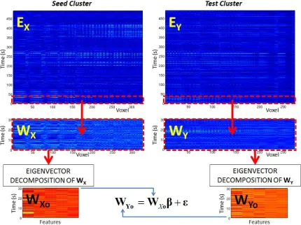
(in seconds) which is allowed to move in time, and we only assess temporal correlation between clusters within these windows. This concept is shownX
o
Y
10
graphically in Figure 1 where the red dotted lines represent the window boundaries. The windowedseed cluster envelope matrix is denoted as
W
X (which has dimension f
Ns) and the windowed test cluster envelope matrix asW
Y(which has dimension f
Nt). Having selected a window, we test for a relationship between the seed and test clusters using a multivariate general linear model, in exactly the same way as described above (Equation 7). Here however, note that we are testing for a linear relationship between the amplitude envelopes of the signal, and not for a linear zero-time-lag relationship between the raw signals.As with leakage reduction, we first account for the fact that separate columns of
W
X orW
Y arelikely to be correlated; again recall that these columns represent envelope timecourses from reconstructed voxels in close spatial proximity. In order to remove this redundancy, and to constrain the degrees of freedom of our test (which will impact on the length of the time window) we decompose these data in a fixed number (d) of orthogonal spatial modes. There are multiple methodologies to impose orthogonality and here eigenvalue decomposition was employed. The
covariance matrices for
W
X andW
Y were computed as:T T
X X X X
XW V T V
W [10]
T T
Y Y Y Y
YW V T V
W [11]
The columns of
V
X andV
Y, which represent the eigenvectors of the covariance ofW
X andW
Yrespectively, were then truncated, leaving only d eigenmodes. Following this, two new matrices are constructed such that:
XT X
Xo W V
W [12]
YT Y
Yo W V
W [13]
Where WXo and WYohave d columns and f
rows. It is important to note here that at least 4d independent temporal observations are required for the multivariate test to be reliable; and this sets the trade-off between the number of spatial features examined and window length ( ). Theorthogonal nature of the columns in WXo and WYo facilitates unambiguous application of the
multivariate GLM such that: ε
β W
WYo Xo [14]
Where β is the matrix of regression coefficients best predicting WYo from WXo. This procedure is
11
Figure 1: Schematic diagram of the windowed multivariate GLM to test for temporal correlation between band limited amplitude envelopes. The time window, represented by the red dashed lines, allows us to measure functional connectivity as a function of time.
Following computation of β, it is possible to apply previously established CCA methods (Soto et al.,
2009, Soto et al., 2010, Barnes et al., 2011, Brookes et al., 2012b). We first compute the covariance
explained by the estimate WXoβ as:
W
β
W
β
H
Xo T Xo [15]In addition, one can compute the unexplained covariance as:
W
W
β
W
W
β
R
Yo
Xo T Yo
Xo [16]It then becomes possible to compute the matrix
H R
D 1 [17]
which corresponds to the ratio of the explained covariance to unexplained covariance. In a
univariate sense, this is equivalent to an F-statistic. In the multivariate case, the eigenvalues,
S
D,and the associated eigenvectors,
A
, ofD
are defined thus: 1
AS A
[image:11.595.82.513.76.398.2]12
The individual columns ofA
(i.e. the eigenvectors) are known as the canonical vectors in WXo andshow explicitly how to combine the individual orthogonal columns of WXo to best explain the
variance observed within and across the columns of WYo. In a similar way the canonical vectors in
Yo
W can be computed as: βA
B [19]
The canonical vectors
A
andB
can be used to calculate the canonical variates; these comprise thecomposite timecourses; that is to say the weighted sum of the columns of WXo and WYo that
maximise temporal correlation, in the window of interest, between the seed and test clusters. The
canonical variates in WXo are given by WXoB and the canonical variates in WYo are given by
A
WYo . It then becomes possible to compute the canonical correlation coefficients thus:
1
W B W A W B W B W A W A
rcan Xo T Yo Xo T Xo Yo T Yo [20]
(Note that the square root represents an element by element square root.) The matrix rcan has
dimension
d
d
and the elements represent correlation coefficients between the various eigenmodes of correlation. As the eigenmodes are, by definition, orthogonal all off-diagonal elements in this matrix are zero and the diagonal elements represent a single canonical correlation coefficient per eigenmode. For the majority of this paper we focus on the first eigenmode (in which most of the variance is explained), but there is no reason why other modes could not be examined (given that the first mode is significant, see figure 6).Finally, the canonical vectors can be projected back onto the individual voxels within the seed and test locations. This generates images showing the optimal weighted sum of voxels in the seed cluster that maximally correlate with the optimal weighted sum of voxels in the test cluster. The voxel weightings in the seed location are given by:
T
X WX AV
I [21]
Likewise the voxel weightings in the test cluster are given by:
T
Y WY BV
I [22]
The above theoretical treatment of beamformer projected MEG data allows for computation of the
canonical correlation coefficient within each time window, along with images, IWX and IWY which
13
2.4) Statistical testing via phase randomisation:
Application of windowed CCA requires careful statistical testing since spurious changes in the temporal profile of correlation can be generated simply as a result of changes in the Fourier components contained within the envelope signals. For example, consider two separate time
windows, A and B; in time window A the windowed envelope signals
W
X andW
Y containcorrelated Gaussian noise (i.e. exhibit an even distribution across all Fourier components), whereas in time window B those envelope data become coloured (i.e. dominated by a small number of Fourier components). In such a case, the number of temporal degrees of freedom in the data is
reduced, and the value of the canonical correlation coefficients rcan will necessarily increase. This
increase is due entirely to the change in spectral structure of the signals and does not represent a genuine change in functional connectivity between the two clusters. Put another way, the background temporal structure in the envelope data will yield non-zero source space correlations that will fluctuate significantly, even if all parameters relating to functional connectivity itself are stationary. For this reason, a robust and reliable statistical technique to account for these ‘trivial’ changes in functional connectivity must be employed.
The technique used here involves generating surrogate envelope data based upon a phase randomisation process; the reader should note that this theory has been well described elsewhere (Prichard, 1994) and is reviewed here for completeness. For univariate data, phase randomisation is a simple procedure in which, given a univariate time series, w(t), we first compute its discrete Fourier transform F
w(t)
A(f)ei(f) where F denotes a Fourier transform, A(f) is the amplitude of each Fourier component and (f) is the phase. A phase randomised signal, w~(t) can then be generated by rotation of the phase of each Fourier component by a random angle, (f), which is chosen uniformly in the range 0 < < 2 (note that (f) differs for each rotated Fourier component). Mathematically, the phase randomised signal is then given as:
( ) ( )
1) ( )
(
~ i f f
e f A F t
w [23]
Note that w~(t) has the desirable property that the magnitude of all of the Fourier components (i.e. the power spectrum) is the same as for the original data, and by the Wiener-Khintchine theorem (Prichard, 1994) so is the autocorrelation function.
Equation [23] describes a univariate case, however
W
X andW
Y are multivariate measurements.In the multivariate case, we not only wish to preserve the Fourier properties of a timeseries, but also
14
preserve the structure of the covariance matrices WXTWX and WYTWY. This can also be achievedvia phase randomisation, if the same random sequence (f) is added to each Fourier transformed
timecourse (i.e. each Fourier transformed column of
W
X andW
Y). Mathematically:
( )
1) ( )
(
~ i f
j j t F F w t e
w [24]
where
w
j(
t
)
represents the jth column ofW
X orW
Y;w
~
j(
t
)
represents the equivalent jth
column
of a surrogate matrix, which we term
W
~
X orW
~
Y. Note that, when constructed in this way,W
~
X andW
Y~
each individually contain the same power spectra and cross correlation structure as
W
Xand
W
Y respectively. However, the phase randomisation means that there should be no correlationbetween
W
X~
or
W
Y~
. This being the case, iterative construction of successive realisations of
W
X~
and
W
Y~
allow for generation of a null distribution, independently for each time window considered
by the windowed CCA. This, in turn, allows for the generation of a dynamic statistical threshold, formed independently for each time window, which accounts for trivial correlations caused by changes in the Fourier components of the envelope signals.
3) SIMULATIONS:
The theoretical analyses described above were applied in simulation to test the applicability of the technique. All simulations were based on the geometry and data collection parameters of the third order synthetic gradiometer configuration of a 275 channel CTF whole head MEG system (MISL, Coquitlam, Canada) with 5cm baseline axial gradiometers. The brain anatomy and head location were based on a real experimental recording session and the simulated sampling rate was 600Hz. In all cases a multiple local sphere volume conductor head model (Huang, 1999) was employed and the forward solution was based on the dipole model derived by Sarvas (Sarvas, 1987).
3.1) Null simulation and leakage reduction:
3.1a) Methodology:
15
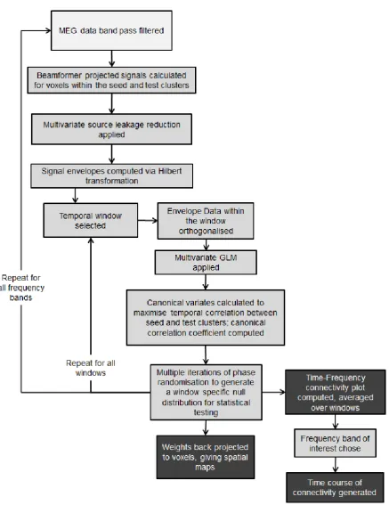
genuine (MEG measured) electrophysiological signals (490s in duration), which were estimated from the motor cortex of a single individual during a resting state experiment. Univariate phase randomisation, as described by Equation 23, was applied in order to maintain the measured power spectral distribution of the neural oscillatory signal, whilst destroying any genuine correlation that might exist between the neural signals used. In this way, no interaction was expected between any of the six simulated sources, meaning that if significant interactions were observed they were entirely spurious and likely due to signal leakage. Signals were frequency filtered to the beta band and all sources were given an amplitude of 3nAm. Note that beta oscillations were used since previous work has shown that the strongest interactions between the left and right sensorimotor areas occur in this frequency band (Brookes et al., 2011a). The simulated dipole timecourses were projected through forward solutions for each dipole location/orientation and summed, yielding a simulated sensor space signal matrix. Additive noise data were generated by experimental recording. A 490s MEG recording was made using the third order synthetic gradiometer configuration of a 275 channel CTF MEG system at a sampling rate of 600Hz, with no subject in the scanner. These ‘empty room’ data formed the noise matrix which was added to the signal matrix thus generating a simulated MEG data set. The signal to noise ratio, defined as the ratio of the Frobenius norm of the signal matrix to the Frobenius norm of the noise matrix, was calculated as 1.6.Having simulated MEG data, the beamformer and CCA techniques were applied as described in Section 2 and summarised in Figure 3. Beamformer projected timecourses were reconstructed on an 8mm grid within regions of interest covering the bilateral sensorimotor cortices. Those regions of interest are shown by the green overlay in Figure 2 and contained all six simulated sources. The seed cluster (containing 327 voxels) covered approximately the left motor strip and the test cluster (containing 274 voxels) covered approximately the right motor strip. Sliding window CCA was applied to source projected data in the beta band only, with a window width () of 30s. The window
was allowed to shift in time by
t
2
s
, giving a total of 230 overlapping windows. The dimensionality (d) of the signals following eigenvalue decomposition of the windowed envelope16
Figure 2: Locations of simulated dipoles in the brain are shown by the blue overlay. The green overlay shows the volume covered by the seed and test voxel clusters.
In order to test the statistical significance of the canonical correlation coefficients computed, multivariate phase randomisation, as described by Equation 24, was employed. For each window, 1000 realisations of the randomised phase matrix ((f)) were employed in order to generate
surrogate matrices
W
X~
and
W
Y~
. The CCA technique was then applied to these surrogate matrices
in exactly the same way as that used for the real
W
X andW
Y. In this way a null distribution ofcorrelation coefficients was generated independently for each time window. The upper 5th percentile was then computed with Bonferroni correction for multiple comparisons across independent time windows (each window was 30 sec from a total of 490 sec and hence a Bonferroni correction of 490/30 was applied). This was then used as a dynamic statistical threshold. This simulation was repeated with and without signal leakage reduction.
17
18
3.1b) Results:
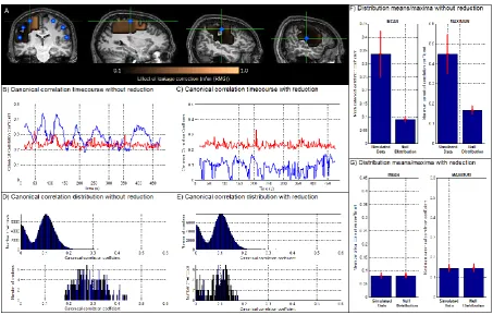
Figure 4A shows a spatial map, highlighting the effect of leakage reduction on each voxel in the test cluster. The coloured overlay shows the magnitude of the mean square difference between the
uncorrected
Y
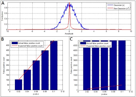
and corrected Yc test matrices, plotted across all voxels within the cluster. It isinteresting to note that the effects of leakage vary spatially, with the largest effects observed in voxels closest to the seed cluster, as would be expected. Figures 4B and 4C show the timecourse of windowed canonical correlation (blue) for data with (4C) and without (4B) reduction of signal leakage. The dynamic statistical threshold (pcorrected=0.05), generated by phase randomisation, is shown in red for both cases. Recall that this is a null simulation, with no expected coupling between sources and so the canonical correlation coefficients in the simulated data should remain below the statistical threshold. This is clearly the case for data with leakage reduction, but it is not the case for data without leakage reduction, where (spurious) significant coupling between voxels in the seed and test clusters is induced exclusively as a result of leakage. Figures 4D and 4E show histograms of canonical correlation coefficients; histograms in the upper panel were derived using phase randomised (null) data and histograms in the lower panel were derived directly from simulated data. Note that the upper panels in Figures 4D and 4E appear identical as the process of phase randomisation implicitly removes any leakage. Again the effect of leakage reduction is obvious, with no observable difference between histograms in the case where correction is applied.
19
Figure 4: Null simulations and the effect of leakage reduction. A) Spatial map showing the mean effect of leakage reduction
on signals at each voxel. The colour overlay represents the mean square difference between the uncorrected
Y
andcorrected Ycmatrices, averaged across all time and plotted across voxels; notice that the largest effects of signal leakage
are distal to the sources, which are marked by the blue dots. B) and C) show timecourses of canonical correlation for simulated data (blue) and the pcorrected=0.05 dynamic statistical threshold (red). The case without leakage reduction is shown
in B and with leakage reduction is shown in C. D) and E) show histograms of canonical correlation coefficients. The upper plots show null distributions derived using phase randomisation. The lower plots show distributions from simulated data. Note that without leakage reduction (D) the mean canonical correlation computed using the simulated data is higher than the null distribution; since no temporal correlation has been simulated in this case, this is an example of spurious correlation. Note also that with leakage reduction (E), the canonical correlation for the simulated corrected data is very similar to the null distribution, highlighting the fact that leakage reduction eliminates the spurious correlations shown in (B). F) and G) show mean and maximum canonical correlation coefficients across 100 iterations of the null simulation (error bars show standard deviation). Note again the difference between the cases with (G) and without (F) leakage reduction.
3.2) Proof of Principle Simulation:
3.2a) Method:
20
cortex of a single individual during a resting state experiment. These were frequency filtered into the 13-30Hz band. Temporal correlation between two sources was simulated within specific time windows, via multiplication by a modulatory function. To illustrate this mathematically, consider the case of two sources, labelled a and b. To impose coupling, we employ the following formulae:)
(
)
(
)
(
1 2 _ 1 2_correlated
a uncorrelated
ab
a
t
t
s
t
t
M
s
[25])
(
)
(
)
(
1 2 _ 1 2_correlated
b uncorrelated
ab
b
t
t
s
t
t
M
s
[26]Here,
s
a_uncorrelated ands
b_uncorrelated represent the simulated neural signals for sources a and brespectively, in the absence of coupling. The window
(
t
1
t
2)
designates the timing of the transient coupling between a and b. Mab(
) is a modulatory function which simulates temporalcorrelation and
s
a_correlated ands
b_correlated represent the transiently coupled timecourses. Mab(
) was derived from a real MEG recording, and comprised genuine 70s segments of a beta band amplitude envelope, extracted via beamforming from the motor cortex of a single subject in the resting state (data from (Brookes et al., 2011a)). There were 6 simulated sources (labelled 1-6 in Figure 2); coupling between sources 5 and 2 was simulated in the time window 50s<t<120s; coupling between sources 3 and 4 was simulated in the time window 200s<t<270s; coupling between sources 1 and 6 was simulated in the time window 350s<t<420s. This generated three coupled source pairsdefined by three independent modulatory functions M52(
), M34(
) and M16(
). This methodology induces a transient (partial) temporal correlation between the amplitude envelopes of the source pairs, within the time windows specified.21
3.2b) Results:
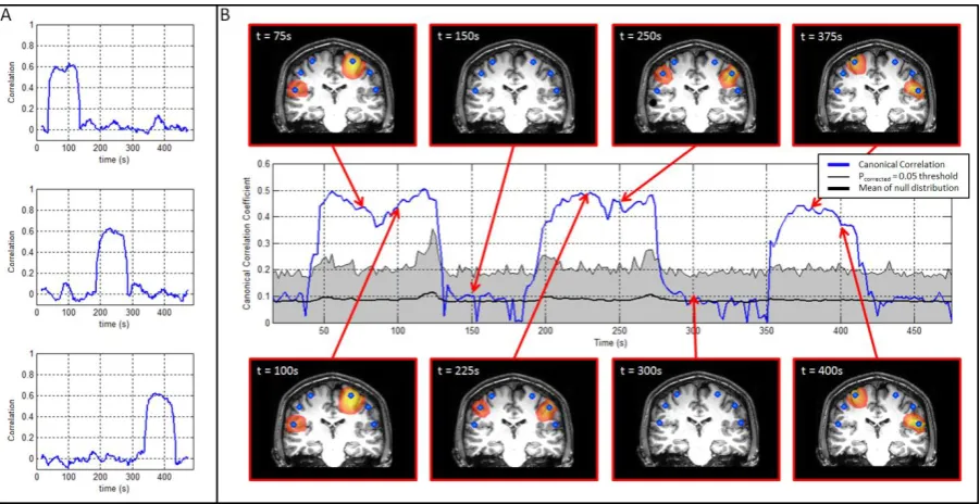
Figure 5 shows results of the proof of principle simulation. Figure 5A represents the ground truth: that is, the temporal evolution of coupling between the simulated timecourses. The upper panel shows correlation between sources 5 and 2, the centre panel correlation between sources 3 and 4, and the lower panel correlation between sources 1 and 6. Note that the technique described by Equations 25 and 26 only induces a partial correlation between source pairs, with the magnitude of that correlation reaching an average of approximately 0.6 (Pearson correlation coefficient) within the windows of transient coupling. Figure 5B shows the estimated canonical correlation as a function of time. The centre timecourse (blue line) shows the reconstructed temporal evolution of canonical correlation between the seed and test clusters. Note that since all six sources exist within the clusters, correlation between all three coupled source pairs is captured in a single timecourse. The thin black line shows the dynamic statistical threshold (pcorrected=0.05) and the thick black line shows the mean of the null distribution (generated via phase randomisation) for each time window. Note that all three simulated interactions yield a significant result in the windowed CCA output. Interestingly, the dynamic statistical threshold also shows temporal structure with the mean of the null distribution, and the pcorrected = 0.05 threshold, changing in time. These changes are driven by temporal structure in the autocorrelation of the envelope timecourses. The spatial maps above and
below the timecourse show individual images (derived from IWX and IWY) depicting the spatial
signature (canonical vectors) of correlation between the left and right clusters. These spatial maps are shown based on 30s time windows centred at t = 75s, 100s, 150s, 225s, 250s, 300s, 375s and 400s. Note that the change in spatial signature as a function of time is in agreement with the simulated connectivity. The blue dots show the locations of the simulated sources.
It should be noted that CCA is a multi-variate methodology and the output for each window is not a single value of canonical correlation, but rather multiple values, each reflecting a separate
eigenmode of correlation (the number of modes is given by the minimum rank of WXo, WYo; in
22
Figure 5: Results of the proof of principle simulation. A) Shows the temporal evolution of simulated connectivity computed using timecourse data. The upper panel shows the timecourse of connectivity between sources 5 and 2; the centre panel shows the timecourse of connectivity between sources 3 and 4; the lower panel shows the timecourse of connectivity between sources 1 and 6. B) Connectivity reconstructed using CCA. The centre timecourse shows the reconstructed temporal evolution of connectivity between the seed and test clusters in the left and right motor strip respectively. Periods of significant temporal correlation are highlighted by the blue line passing outside the shaded region, which is bounded by a pcorrected=0.05 statistical threshold derived independently for each window, and corrected for multiple time windows. The
thick black line shows the mean canonical correlation for the null distribution, generated via phase randomisation. The
spatial maps show individual images (i.e. IWX and IWY) depicting the spatial signature (canonical vectors) of correlation
[image:22.595.76.517.523.652.2]between the left and right clusters. Note the change in spatial signature as a function of time is in agreement with the simulated connectivity. The blue dots show the locations of the simulated sources.
23
4) REAL MEG DATA
4.1a) Methodology: data acquisition
Following application of windowed CCA in simulation, the same technique was applied to real MEG data. Data were acquired at a sampling rate of 600 Hz using the third order synthetic gradiometer configuration of a 275 channel MEG system (MISL, Coquitlam, Canada) with a 150Hz low pass anti-aliasing filter. Subjects were asked to lie (supine) in the MEG system, with their eyes open and ‘rest’ whilst 600s of extra-cranial magnetic field data were acquired. Prior to the recording, three localisation coils were attached to the head as fiducial markers (nasion, left preauricular and right preauricular). Energising these coils during data acquisition enabled localisation of the head relative to the MEG sensors. In order to co-register the MEG sensor geometry to the brain anatomy, the subject’s head shape was digitised (Polhemus Isotrack) relative to the fiducial markers. MR images were acquired using a 3T Phillips Achieva MR system running an MPRAGE sequence at 1x1x1mm3 resolution. Coregistration was then achieved by matching the digitised surface to the head surface extracted from the subject’s volumetric anatomical MR image. This experimental procedure was approved by the local research ethics committee.
4.1b) Methodology: data analysis
The recorded MEG data were inspected visually and segments containing excessive noise removed. These data were then processed using the technique described in Section 2 and summarised in Figure 3. Seed and test clusters were defined covering the left and right sensorimotor areas respectively; these regions are highlighted by the green overlay in Figure 7A. Beamforming was applied in order to reconstruct timecourses of electrical activity on an 8mm cubic grid spanning the seed and test clusters. The beamforming and CCA method (Figure 3) was applied iteratively (treating each band independently) over multiple overlapping frequency bands (4-8Hz, 6-10Hz, 8-13Hz, 10-15Hz and subsequent overlapping windows (10Hz bandwidth, 5Hz overlap) up to 105Hz). For each band we used a fixed window width () of 40s, a total of 280 windows, and a dimensionality (i.e. d,
the number of columns in WXo and WYo) of 3. The values of the canonical correlation coefficients,
computed independently for each time window and frequency band, were used to construct a time-frequency (t-f) connectivity plot.
Having computed canonical correlation across all frequencies, a single band of interest was identified for further analysis. MEG data were filtered in the 10-35Hz band and again beamforming was applied to reconstruct timecourses on an 8mm cubic grid spanning the seed and test clusters.
24
window. For each window, IWX and IWY (which represent the seed and test clusters respectively)were combined into a single image, thus generating a total of 280 separate spatial maps, each showing the weightings for voxels (canonical vectors) in the left and right sensorimotor region that describe optimal correlation between clusters. A timecourse of canonical correlation coefficients was also generated, and the significance of each coefficient computed using the phase randomisation approach, with correction for multiple comparisons across independent windows applied using the Bonferroni method. Although separate timecourses and image sets can be computed for each canonical mode, in this example only the dominant mode is considered.
The set of 280 volumetric images (one per time window) show changes in the spatial signature of functional connectivity. However visualisation of this set of images is not trivial. In cases where a task has been employed, one might pick particular time windows that correspond to specific aspects of the task. In the present case however, since the MEG data represent subjects in a ‘resting’ state, any selection of time windows is somewhat arbitrary. A new set of problems therefore arise – how to identify the number of significantly different canonical vectors or spatial modes. For simplicity we collapsed our 280 images into a smaller number of spatial patterns. To do this, first a covariance matrix was constructed, with dimension
280
280
whose ijth element contained the spatial covariance of image i with image j. This matrix was then decomposed into its constituent eigenvectors and eigenvalues. The eigenvectors were multiplied by the images in order to generate volumetric maps showing the spatial signature of each eigenmode; these maps are henceforth termed spatial modes and effectively represent orthogonal spatial patterns of connectivity observed within the 280 image set. The eigenvectors represent the weighting of each individual time window to a particular spatial mode, and can be thought of as a time series showing the contribution of each time point to that mode.4.2) Resting state MEG data: Results
8-25
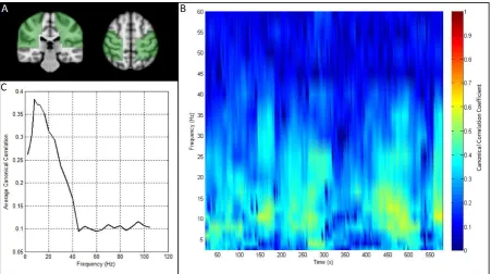
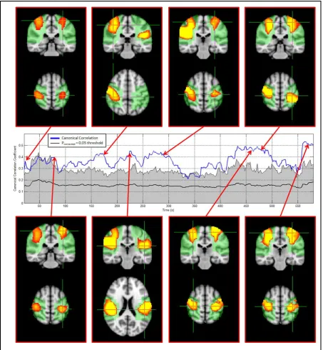
35Hz frequency band. This is also evidenced by Figure 7C, which shows the time average of canonical correlation plotted as a function of frequency.The temporal and spatial variation of connectivity in the 10 – 35Hz frequency band is shown in Figure 8. The centre timecourse (blue line) shows the reconstructed temporal evolution of canonical correlation between the seed and test clusters in left and right sensorimotor cortices respectively. The thin black line shows the dynamic statistical threshold (pcorrected=0.05) and the thick black line shows the mean of the null distribution (generated via phase randomisation) for each time window. Note that, in agreement with other results (de Pasquale et al., 2010, Baker et al., 2012) there is significant temporal variation in resting state correlation. As with the simulated data, the dynamic statistical threshold and mean canonical correlation calculated for the null distribution shows significant temporal structure. This temporal structure shows that a degree of temporal variability in metrics of functional connectivity can be generated purely as a result of changes in the Fourier component that make up the source timecourses in a given window.
26
Figure 7: Resting state motor network connectivity. A) Green overlays show the anatomical locations of the seed and test clusters, in left and right sensorimotor regions respectively. B) Time frequency connectivity plot showing the temporal and spectral evolution of band limited amplitude correlation between voxel clusters in the left and right sensorimotor regions. C) Average connectivity spectrum, showing that the highest average motor network connectivity occurs in the alpha and beta bands.
27
Figure 8: Spatial patterns of connectivity in the 10 – 35Hz frequency band. The centre (blue) timecourse shows the reconstructed temporal evolution of connectivity between the seed and test clusters in the left and right motor strip respectively. Periods of significant temporal correlation are highlighted by the blue line passing outside the shaded region, which is bounded by a pcorrected=0.05 statistical threshold derived independently for each window (and corrected for multiple
windows). The thick black line shows the mean canonical correlation for the null distribution, generated via phase
randomisation. The spatial maps show coronal and axial aspects of the individual images (i.e. IWX and IWY) depicting
[image:27.595.72.526.71.562.2]28
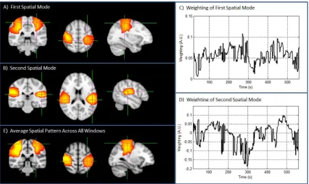
Figure 9: Spatial modes of correlation. A) and B) show the first and second spatial modes of correlation respectively; the timecourses showing the contribution of each time window to the first and second spatial modes are shown in C and D. E) shows the simple time average of all 500 images.
5) DISCUSSION:
The next generation of tools to compute functional connectivity in neuroimaging data must account for temporal non-stationarity, spatial inhomogeneities, and spectral structure. Here, we have presented a means to achieve this via application of beamforming and windowed CCA to MEG data. We have shown it possible to generate time-frequency connectivity plots showing the temporal and spectral evolution of coupling between brain regions. Moreover, CCA over voxels provides a means to assess spatial inhomogeneity within those short time-frequency windows. We have demonstrated the feasibility of this technique in simulation, and using real MEG data.
29
for leakage reduction based on removal of linear (zero-phase-lag) interactions between beamformer projected source time series in the seed and test clusters. Source leakage between voxels in MEG is necessarily zero-phase-lag, and removal of this component has been demonstrated by previous papers (Brookes et al., 2012b, Hipp et al., 2012) as an effective means to reduce spurious interactions. Here we extended the regression idea from the univariate case presented previously (Brookes et al., 2012b, Hipp et al., 2012), to a multivariate case. This extension facilitates removal of linear interactions between all voxels (and all linear mixtures of voxels) in the seed and test clusters. As expected, the magnitude of the effect of this reduction differs across voxels within the clusters; this was shown in Figure 4A, with the largest degree of reduction in voxels located in close proximity to the seed cluster. Empirical evidence for the success of this method was given in Figures 4B – 4G. Without leakage reduction, canonical correlation coefficients between the seed and test cluster were higher in the simulation than for a phase randomised case. Recall that phase randomisation not only destroys genuine correlation (i.e. functional connectivity) but also destroys spurious correlation caused by leakage. This means that prior to leakage reduction, a significant difference in canonical correlation between simulated and phase randomised data would be driven entirely by leakage – this was observed in Figures 4B, D and F. Following leakage reduction however, this difference would be expected to be eliminated, and this was indeed evidenced by Figures 4C, E and G. The empirical evidence presented therefore adds weight to previous studies (Brookes et al., 2012b, Hipp et al., 2012) in showing that regression based leakage reduction is effective in ensuring a correct false positive rate in subsequent connectivity assessment (see also appendix).30
here are unaveraged, making accurate measurement of temporal coupling challenging. CCA, applied across voxels, is helpful in this context since is allows a principled way to generate a weighted average of signals across multiple voxels in source space. Averaging voxel timecourses in this way enables an effective increase in the SNR of the data, and hence a more accurate means to assess the time-frequency evolution of connectivity.Statistical thresholding to define time-frequency windows exhibiting significant temporal correlation is non-trivial. As described in section 2.4, changes in the temporal profile of correlation can be generated simply as a result of changes in the temporal autocorrelation of the envelope time series across multiple time windows. Such temporal structure in the envelope timecourse for the seed and test regions will yield changes in correlation; such changes are trivial, and driven not by a genuine change in functional coupling between regions, but by changes in the Fourier components that make up the signal. In this paper, we apply a previously described technique (Prichard, 1994) to correct for such trivial changes in canonical correlation by employing a dynamic statistical test based on multivariate phase randomisation. By building a null distribution based on Equation 24, we ensure that the canonical correlation coefficients defining that null are constructed using surrogate windowed envelope timecourses with the same autocorrelation function as the real data. This means that any changes in correlation driven purely by changes in signal characteristics are accounted for by the statistical threshold. It is interesting to note that, in real MEG data, this approach yields a dynamic statistical threshold that exhibits marked changes in time. Future work using MEG (or fMRI) to measure dynamic changes in functional connectivity should bear this issue in mind, and consider methods that account for this temporal non-stationarity.
31
by the selected regions (larger regions require increased d) and the spatial resolution of the MEG inverse projection within those regions (higher spatial resolution means more independent signals within a cortical volume, necessitating larger d). This means that, again, selection of d is specific to the particular study being undertaken; this said an objective means to select d can be derived as the percentage of data variance explained by the eigenmodes retained. Finally, judicious selection of a time frequency window involves a trade-off between temporal/spectral resolution and accuracy. The smaller the time frequency window, the less accurate the estimation of canonical correlation. The window size is also related to the number of selected eigenmodes (d) and, as a rule of thumb, one requires more than 4d independent temporal observations within the window for the multivariate test to be reliable. This imposes a fundamental limit on temporal resolution of any sliding window technique. In task based studies, this poses less of a problem since time windows can be made narrow, and the amount of data within a window effectively increased by concatenation of data segments across task trials. However, in the resting state this is not possible. A powerful and complementary alternative to sliding windows, which has particular application in resting state MEG measurements, is to deploy techniques such as Hidden Markov Models (HMMs), which have been shown to detect short-lived re-occurring states in resting state MEG data, characterised by repeating patterns of covariance over channels (Woolrich et al., 2013). This multivariate approach has, so far, been used to perform temporally adaptive MEG source reconstruction and could be readily extended for use with CCA. In addition to these fundamental parameters, windowed CCA as described is critically dependent on source localisation, in this case using beamforming. Parameter selection and optimised application of beamforming is covered extensively in previous literature and will not be reproduced here. However we do note that windowed CCA may, in principle, by applied in conjunction with any inverse projection technique, with the caveat that different inverse projection algorithms exhibit different signal leakage characteristics and the interaction between inverse projection and leakage reduction should be characterised prior to direct application.32
network, with spatially distinct ‘sub-networks’ exhibiting significant canonical correlation within temporally separated windows. This result was extended further in Figure 9, with the inclusion of volumetric maps depicting two separate spatial modes of correlation. The first spatial mode resembles strongly a well-known sensorimotor network, which is often observed in both bilateral and unilateral motor paradigms. This comprises bilateral and symmetric regions covering (approximately) the hand areas of left and right sensorimotor cortex. The second spatial mode incorporates bilateral and symmetric cortical regions observed in inferior slices. The inherent smoothness of MEG images necessarily makes unambiguous spatial interpretation of these images challenging, but nevertheless this secondary spatial mode is physiologically plausible, and may incorporate the bilateral secondary somatosensory region. Similar spatial patterns were found in a second individual during a resting state MEG acquisition. Methods to derive robust and regularly occurring spatial patterns of connectivity offer a means to extend the CCA technique from single subject application (as presented) to group study. Techniques such as eigenvalue decomposition (as used here) or alternatively k-means clustering, should allow elucidation of consistent spatial patterns across multiple subjects. Alternatively, it is conceivable that concatenating spatially normalised volumetric images across many subjects may generate large multi-subject datasets amenable to processing with techniques such as spatial ICA, which again may elucidate robust and regularly occurring spatial patterns of functional sub-networks within (for example) the sensorimotor system. Although it remains to be seen whether or not our present findings extend across large groups of subjects, they do present an immediate example of the utility of the windowed CCA approach. Further work might attempt to provide a principled identification of the number of spatial and temporal modes of correlation supported by MEG data.6) CONCLUSION:
34
7) APPENDIX: LEAKAGE REDUCTION USING LINEAR REGRESSION
The principal limitation of MEG as a means to measure functional connectivity is signal leakage between spatially separate locations. ‘Leakage’ is a result of imperfect source localisation which, in turn, results from the ill posed MEG inverse problem. The leakage reduction methodology that we employ is a post-hoc fix to limit the effect of poor source localisation on functional connectivity. The idea is to reduce linear (zero-phase-lag) interactions between beamformer projected source time series in the seed and test clusters. This is achieved using linear regression (Brookes et al., 2012b,
Hipp et al., 2012), in which we derive a leakage coefficient (
β
L) which can be used subsequently tomodify the estimate of electrical activity at the test location. To gain further insight into the leakage reduction methodology it proves instructive to undertake a simple analytical analysis.
7.1) Analytical analysis
Consider a simple case with two sources, q1 represents the timecourse from our test location (r1) whilst q2 represents the timecourse at the seed location (r2). Assuming no other electrophysiological sources in the brain, the MEG data are described by:
e q l q l
m 1 1 2 2 [A1]
Where l1 and l2 represent the lead field vectors for sources q1 and q2 and e represents sensor level
noise. Now assume that we employ a beamformer to reconstruct an estimate of source q1 so that:
fT m w
qˆ1 1 [A2]
Note that the ‘hat’ notation represents an estimate (i.e. qˆ1 is an estimate of the true source
timecourse q1). w1 represents the beamformer weights for location r1, which are given by
1 1 1 1 1 1 l C l C l w
TT
T
[A3]
Where C is the data covariance matrix. Substituting Equations A1 and A3 into A2, and using the
definition of a beamformer unit constraint (i.e. w1l1 1
T
) we can show that:
2 1 1 1 2 1 1 1 1 ˆ q l C l l C l q q
TT [A4]
So in this case, the magnitude of the leakage from the seed location to the test location is given by:
11 1 1 2 1 1
lTC l lTC l
a [A5]
35
M1 2
1 ˆ ˆ
ˆ q q
q
[A6]Where qˆ1M represents the modified source estimate for q1 following leakage reduction. The
‘leakage parameter,’
, is given by the Moore-Penrose pseudo-inverse of q2, mathematically:
2 11 2 2ˆ ˆ ˆ
ˆ q q q
qT T
[A7]If we assume that qˆ2 is a perfect reconstruction (i.e. qˆ2 q2), and substitute equation A4 and A5
into A6 we find that:
2
1 2
1 2
2q q q q
qT T a
[A8]If q1 and q2 are temporally uncorrelated (a condition for beamforming) such that q1q2 q2q1 0 T T
(this is the case in the infinite integration limit) then:
T
T a T
a 1 2 1 2 2
2
2q q q q q
q
[A9]In other words, given uncorrelated sources and perfect reconstruction of the interfering source q2, the leakage parameter
is an unbiased estimate of the leakage, a. We term this case ‘1-wayleakage’, meaning that we get leakage of q2 into q1, but no leakage from q1 into q2. This condition
may be met if q2 represented a fundamentally different process. For example, the interfering
source, q2, may represent cardiac interference and may be measured using an ECG. In such a case
the magnetocardiogram could easily leak into a beamformer projected MEG signal, but it is unlikely that a MEG signal could leak back into the ECG measurement. This is therefore a likely case of 1-way-leakage.
Unfortunately, for measurements of functional connectivity between two brain regions, the
assumption that qˆ2 q2 will never be met. This is because qˆ2 is a beamformer estimated
timecourse and if we observe leakage of the seed source into the test source (q2 into q1), we are
highly likely to observe leakage of the test source into the seed source (q1 into q2). We term this
more complex case ‘2-way-leakage’. By analogy with Equation A4, in the case of 2-way-leakage, the beamformer estimate of the seed source q2 will be given by:
1 2 1 2 1 2 1 1 2 2 2
ˆ q q q
l C l l C l q
q T b
T
[A10]
Where
2
11 2 1 1 2
lTC l lTC l
b . Substituting Equations A4, A5 and A10 into A7 we get:
2 1
1 2
1 1 2 1
2 q q q q q q q
q b T b b T a
[A11]Again assuming that q1 and q2 are temporally uncorrelated we find that:
2 2 1 1
1 1 1 2 2
2q q q q q q q
qT b T a T b T