Hydrodynamic electron flow and Hall viscosity

Thomas Scaffidi,1 _{Nabhanila Nandi,}2 _{Burkhard Schmidt,}2 _{Andrew P. Mackenzie,}2, 3 _{and Joel E. Moore}1, 4 1_{Department of Physics, University of California, Berkeley, CA 94720, USA}

2

Max Planck Institute for Chemical Physics of Solids, N¨othnitzer Strasse 40, 01187 Dresden, Germany

3_{Scottish Universities Physics Alliance, School of Physics and Astronomy,}

University of St. Andrews, St. Andrews, Fife KY16 9SS, UK

4

Materials Sciences Division, Lawrence Berkeley National Laboratory, Berkeley, CA 94720

(Dated: March 22, 2017)

In metallic samples of small enough size and sufficiently strong momentum-conserving scattering, the viscosity of the electron gas can become the dominant process governing transport. In this regime, momentum is a long-lived quantity whose evolution is described by an emergent hydro-dynamical theory. Furthermore, breaking time-reversal symmetry leads to the appearance of an odd component to the viscosity called the Hall viscosity, which has attracted considerable attention recently due to its quantized nature in gapped systems but still eludes experimental confirmation. Based on microscopic calculations, we discuss how to measure the effects of both the even and odd components of the viscosity using hydrodynamic electronic transport in mesoscopic samples under applied magnetic fields.

The semiclassical theory of electronic conduction, based on relaxation of total momentum by impurities, phonons and umklapp scattering, occupies a central place in condensed matter physics. It is therefore of particu-lar interest to study the cases for which it fails. One case that has attracted much interest is the possibility of a hy-drodynamic regime, where transport is dominated by vis-cous effects [1–22]. One needs a large separation of scales between momentum-relaxing and momentum-conserving scattering in order to see these effects. This was recently achieved in graphene[23, 24] and PdCoO2[25, 26].

Interest in such a hydrodynamic regime also emanated from a conjectured bound on diffusion constants for the hydrodynamics of strongly interacting quantum systems [27, 28]. Even though the physics described in this work is semiclassical and probably still quite far from these quantum-mechanical bounds, the observations that we hope to stimulate would constitute an important first step towards the understanding of emergent hydrody-namical regimes in electronic systems.

A further motivation for the work is that reaching a viscous regime for a charged fluid enables one to break time-reversal symmetry by adding a magnetic field and hence to study a non-dissipative component to the viscos-ity tensor called the Hall viscosviscos-ity. The recent interest in this Hall viscosity emanates from the fact that it is topologically quantized in gapped systems [29]. In or-der to study this effect experimentally, in analogy with the Hall conductivity, the first step would obviously be to measure the classicalHall viscosity. We show in this letter how this measurement could be done by describ-ing specific size effects from Hall viscosity in transport in restricted 2D channels under transverse magnetic fields.

This paper is organized as follows. We start by assum-ing a perfect hydrodynamic regime and calculateρxxand

ρxy. We show that the 1/W2 component of ρxy is

pro-portional to the Hall viscosity, thereby providing a way of measuring it. In order to have realistic predictions to compare with experiments, one should also take into account other, non-viscous effects that can lead to a size-dependent resistivity. We thus perform a kinetic Boltz-mann calculation in which the effect of diffuse bound-aries, gradient along the section of the wire, momentum-conserving scattering, and magnetic field are taken into account. We show that the size effects in resistivities with and without momentum-conserving scattering are markedly different, thereby making it possible to distin-guish hydrodynamic and non-hydrodynamic size effects. Finally, we comment on how these measurements could also enable one to measure the quantum Hall viscosity in the quantum Hall regime and establish a relation similar to Hoyos-Son [30].

FLUID EQUATION

Even though a finite amount of momentum relaxation is always present, it is instructive to first look at the limit where it is zero. In this limit, the momentum density of the electron gas is conserved and one can write a hydro-dynamic equation to model its hydro-dynamics [14] [31]:

∂t~v=ηxx∇2~v+ηxy∇2~v×~z+

e m(

~

E+~v×B~) (1)

where m is the electron mass and ηxx and ηxy are the

regular and Hall components of the kinematic viscosity tensor. As mentioned previously, the two diffusion con-stants in this equation are interesting from a fundamen-tal point of view: (1) from a holographic argument, a bound onηxx was conjectured (coming from the bound

on the dissipative time scale_~/kBT) and (2)ηxy is

non-dissipative (and therefore not subject to this bound) but was shown to be quantized in gapped systems [32–35].

We consider the case of a two-dimensional channel of width W along they direction, with a uniform applied electric fieldExalongx, uniform magnetic fieldB along

z, and zero current along y. In the stationary regime, one finds

ηxx

d2_v

x

dy2 +

e

mEx= 0

−ηxy

d2_v

x

dy2 +

e

mEy =ωcvx

(2)

where ωc = eB/m. Using the conventional no-slip

boundary condition vx(y = ±W/2) = 0 (we will treat

the more realistic case of diffuse boundaries within a ki-netic formalism in the next section), one finds

ρxx=

m e2_nηxx

12

W2

ρxy=ρbulkxy

1−ηxy

12

W2 1

ωc

(3)

where ρbulk

xy = −

mωc

e2_n. In the wide sample limit (W →

∞), one hasρxx= 0, since the only source of resistance

comes from the boundaries, andρxy=−mωc/e2n, which

is indeed its bulk value. We propose to measureηxx and

ηxy by measuring the size dependence of ρxx and ρxy

in restricted channels of varying size and under varying magnetic fields.

In the next section, we will compare these results with the results of a kinetic Boltzman formalism. In order to do so, it is convenient to inject a microscopically derived magnetic field dependence of the viscosities in the above hydrodynamic solutions. The following dependence was found by Alekseev [14]:

ηxx=η

1 1 + (2lM C

rc )

2

ηxy=η

2lM C

rc

1 + (2lM C

rc )

2

(4)

where rc = mvF/eB = vF/ωc is the cyclotron radius,

lM C = vFτM C is the momentum-conserving scattering

length and whereη= 1₄vFlM C [14]. This leads to

ρxx=

m e2_n

12

W2η 1 1 + (2lM C

rc )

2

ρxy=ρbulkxy 1−6

1 1 + (2lM C

rc )

2

_l

M C

W

2! (5)

The size effect on ρxy is maximal at zero field due to

the Lorentzian factor. In this limit, one obtains

ρxy=ρbulkxy 1−6

_l

M C

W

2!

forB →0 (6)

In order to measure this effect,W should be as small as possible for it to be sizable, but still somewhat larger than

lM C in order to remain in the hydrodynamic regime. For

example, forW/lM C = 5, one expects a relative change

of the Hall slope at zero field of the order of 25%, which should be measurable.

KINETIC THEORY

As mentioned previously, in order to make a quanti-tative comparison with experiments, it is crucial to go beyond a purely hydrodynamical theory and take into account several other effects like the non-zero momen-tum relaxation and the diffuse scattering at the bound-aries. In order to do this, we perform kinetic Boltzmann calculations [8, 25, 36]:

~

v· ∇~rf+

e

m(E+~v× ~

B)· ∇~vf =

∂f ∂t _scatt (7)

whereB~ is the external magnetic field,f(~r, ~v) is the semi-classical occupation number for a wavepacket at position

~rand velocity~v and where

∂f(~r, ~v)

∂t

_scatt

=−f(~r, ~v)−n(~r)

τ +

2

τM C

~v·~j(~r) (8)

withn(~r) =hfi_~v the local charge density,~j(~r) = hf~vi_~v the local current, h. . .i_~v the momentum average and

τ−1=τ_{M R}−1 +τ_{M C}−1. For the sake of simplicity, we consider the case of a circular Fermi surface with~v=vFρˆwith ˆρ

the radial unit vector. Scattering lengths are then simply defined aslM R(M C) = vF τM R(M C). The term propor-tional toτ_{M C}−1 is the most simple momentum-conserving scattering term that can be written assuming that the electrons relax to a Fermi-Dirac distribution shifted by the drift velocity [7, 25]. The boundary conditions are given by

jy(y=±W/2) = 0

f(y=±W/2, ~v) =±fboundary

(9)

which imposes, respectively, no current in theydirection and diffuse scattering at the boundaries. Equation 7 is supplemented by Gauss’s law with a charge density given by en(~x). The resulting integrodifferential equation is advantageously solved numerically by using the method of characteristics [37].

Three limiting regimes can be identified [8]: Ohmic, hydrodynamic and ballistic. In the Ohmic case, one has lM R W, and transport is therefore dominated

by momentum-relaxing scattering, leading to bulk values for transport coefficients: ρxx=ρbulkxx =m/ne2τM Rand

ρxy =ρbulkxy =−mωc/e2n. In the ballistic case, one has

W lM R, lM C, and transport is dominated by

in the hydrodynamic regime. Finally, in the hydrody-namic case, one haslM C W lM R, and transport is

dominated by the diffusion of momentum at the bound-aries through viscosity. Note that this regime will only appear iflM ClM R.

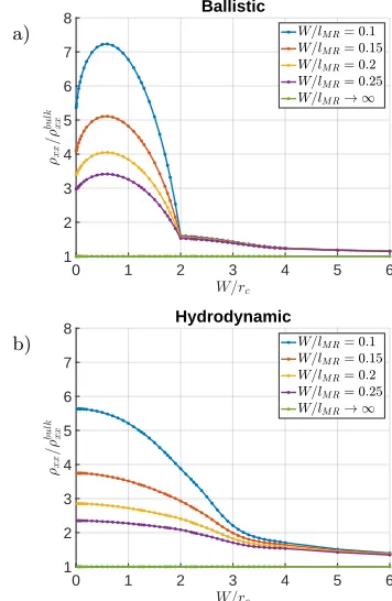
Using the above kinetic theory, we look at transport in and between these different regimes and identify clear signatures of a hydrodynamic regime. In figures 1 and 2, we give respectively the magnetoresistance and the Hall resistivity in a typical ballistic case (lM C/lM R= 10,W .

lM R) and a typical hydrodynamic case (lM C/lM R= 0.05,

lM C < W < lM R).

In the ballistic regime (Fig 1.a), the magnetoresistance shows a maximum around W/rc ' 0.55 and a rapid

change of slope at W/rc = 2, as previously reported

[36, 38]. In this ballistic regime, transport is dominated by electrons with a velocity close to the longitudinal (ˆx) direction for which scattering on boundaries are very rare. These trajectories are bent by the field, leading to an increase in boundary scattering and therefore an increase of ρxx at low fields. At higher fields, when the

cyclotron radius becomes of the order ofW, a larger and larger fraction of electrons present near the middle of the wire stop seeing the boundaries at all, and at large fields the bulk resistivity is therefore recovered.

In contrast, in the hydrodynamic regime (Fig 1.b), the longitudinal magnetoresistance decays monotonically and there is no sharp slope change at W/rc = 2. The

magnetoresistance follows a Lorentzian-like curve, in agreement with the hydrodynamic calculation of Eq. 5. This absence of sharp behavior atW/rc= 2 shows that,

in this case, momentum-conserving scattering is domi-nant and no electron can ever go over a full cyclotron or-bit without being scattered. As explicit in Eq. 5, the rel-evant dimensionless parameter is therefore nowlM C/rc,

as opposed toW/rcin the ballistic case. The absence of a

maximum of the magnetoresistance and of a sharp slope change at W/rc = 2 can be used as clear signatures of

the hydrodynamic regime. Note that the different scaling of ρxx withW in zero applied field can also be used to

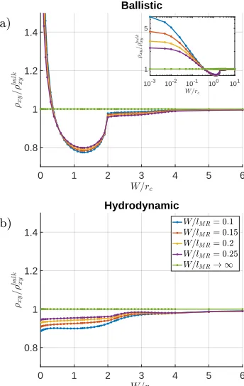
differentiate the two regimes, as reported in [25]. The Hall resistivity also shows strikingly different be-haviors in the ballistic and hydrodynamic regimes. As seen in Fig. 2.b, in the ballistic case, ρxy exhibits a

minimum at W/rc ' 1.3 and a sharp slope change at

W/rc = 2, in analogy with ρxx and in agreement with

the perturbative calculation given in Ref. [39]. While, in the ballistic case, ∆ρxy ≡ ρxy−ρbulkxy is positive at low

fields and negative at large fields, it is always negative in the hydrodynamic case (see Fig 2.b). The sign of ∆ρxy

can therefore be used a clear signature of hydrodynamic effects: one would expect a smaller (resp. larger) Hall slope at small fields than at large fields in the hydrody-namic (resp. ballistic) regime.

It was checked that, in both the cases oflM C/lM R= 10

and lM C/lM R = 0.05, if W becomes larger than lM R,

0 1 2 3 4 5 6

1 2 3 4 5 6 7

8 Ballistic a)

0 1 2 3 4 5 6

1 2 3 4 5 6 7

8 Hydrodynamic b)

FIG. 1. Magnetoresistance for the ballistic (lM C/lM R= 10)

(a) and hydrodynamic case (lM C/lM R= 0.05) (b).

Ohmic behavior is recovered. It was also checked that, in the case of lM C/lM R = 0.05, if W becomes smaller

thanlM R, ballistic behavior is recovered.

QUANTUM LIMIT

While the calculations up to this point have been clas-sical, it is instructive to look at the large magnetic field limit, rc/lM C →0. In this limit, one finds from Eq. 4

that

ηxy→

1

8vFrc (10)

which, crucially, does not depend on lM C. Now, using

ν = 2πl2

Bn, vF = ~kF/m with kF =

√

4πn and l2

B =

~/eB, one finds

˜

ηxy=nmηxy=

1 8π

~ν2 l2

B

(11)

which gives the quantized value of the dynamical viscos-ity ˜η for a quantum Hall system at filling ν. Inverting the resistivity tensor obtained in Eq. 3 and taking the large field limit leads to the conductivity:

σxy=ν

e2

h

1 +η˜xy ~n

(qefflB)2

2π/qeff= 2πW/ √

12'1.8W

0 1 2 3 4 5 6 0.8

1 1.2 1.4

Ballistic

10-3 10-2 10-1 100 101 1

5 a)

0 1 2 3 4 5 6

0.8 1 1.2 1.4

Hydrodynamic b)

FIG. 2. Hall resistivity for the ballistic (lM C/lM R= 10) (a)

and hydrodynamic case (lM C/lM R= 0.05) (b). The inset of

panel (a) shows the saturation of the Hall resistivity at low fields in the ballistic case.

The large magnetic field extrapolation of the classical cal-culation found in this paper is therefore consistent with the form of the finite-q correction found by Hoyos and Son in the quantum case [30] [40]. In the quantum Hall regime, the relative deviation ofσxyfrom its bulk value is

of the order ofν2_(q

efflB)2. For realistic system sizes, the

factor (qefflB)2 would probably be too small to lead to

a measurable deviation. One could then turn to optical probes whereqeff could be chosen in the X-ray range.

CONCLUSION

In conclusion, we have identified clear, qualitative sig-natures of hydrodynamic behavior in transport measure-ments of mesoscopic metallic samples under magnetic fields. This type of measurement is possible with read-ily available experimental techniques, and would make it possible to measure the classical Hall viscosity of the elec-tron gas, which to the best of our knowledge has never been measured in a solid-state system. This would both further the evidence of a hydrodynamic regime in elec-tronic transport and constitute an important step to-wards an experimental understanding of the quantum Hall viscosity.

ACKNOWLEDGEMENTS

Helpful conversations with Tankut Can and Sriram Ganeshan are acknowledged. The authors acknowledge support from the Emergent Phenomena in Quantum Sys-tems initiative of the Gordon and Betty Moore Founda-tion (T. S.) and NSF DMR-1507141 and a Simons In-vestigatorship (J.E.M.). We also acknowledge the sup-port of the Max Planck Society and the UK Engineer-ing and Physical Sciences Research Council under grant EP/I032487/1.

[1] R. Gurzhi, Sov. Phys. JETP44, 771 (1963). [2] R. Gurzhi, Physics-Uspekhi11, 255 (1968). [3] J. E. Black, Phys. Rev. B21, 3279 (1980).

[4] Z. Z. Yu, M. Haerle, J. W. Zwart, J. Bass, W. P. Pratt, and P. A. Schroeder, Phys. Rev. Lett.52, 368 (1984). [5] R. Gurzhi, A. Kalinenko, and A. Kopeliovich, Physical

review letters74, 3872 (1995).

[6] L. Molenkamp and M. De Jong, Solid-state electronics

37, 551 (1994).

[7] L. W. Molenkamp and M. J. M. de Jong, Phys. Rev. B

49, 5038 (1994).

[8] M. J. M. de Jong and L. W. Molenkamp, Phys. Rev. B

51, 13389 (1995).

[9] M. Dyakonov and M. Shur, Phys. Rev. Lett. 71, 2465 (1993).

[10] E. Chow, H. P. Wei, S. M. Girvin, and M. Shayegan, Phys. Rev. Lett.77, 1143 (1996).

[11] B. Spivak and S. A. Kivelson, Annals of Physics321, 2071 (2006).

[12] A. V. Andreev, S. A. Kivelson, and B. Spivak, Phys. Rev. Lett.106, 256804 (2011).

[13] I. Torre, A. Tomadin, A. K. Geim, and M. Polini, Phys. Rev. B92, 165433 (2015).

[14] P. S. Alekseev, Phys. Rev. Lett.117, 166601 (2016). [15] A. Tomadin, G. Vignale, and M. Polini, Phys. Rev. Lett.

113, 235901 (2014).

[16] L. Levitov and G. Falkovich, Nat Phys12, 672 (2016). [17] M. Sherafati, A. Principi, and G. Vignale, Phys. Rev. B

94, 125427 (2016).

[18] H. Guo, E. Ilseven, G. Falkovich, and L. Levitov, ArXiv e-prints (2016), arXiv:1607.07269 [cond-mat.mes-hall]. [19] H. Guo, E. Ilseven, G. Falkovich, and L. Levitov, ArXiv

e-prints (2016), arXiv:1612.09239 [cond-mat.mes-hall]. [20] A. Lucas, ArXiv e-prints (2016), arXiv:1612.00856

[cond-mat.mes-hall].

[21] A. Levchenko, H.-Y. Xie, and A. V. Andreev, ArXiv e-prints (2016), arXiv:1612.09275 [cond-mat.mes-hall]. [22] S. Ganeshan and A. G. Abanov, ArXiv e-prints (2017),

arXiv:1703.04522 [physics.flu-dyn].

[23] D. A. Bandurin, I. Torre, R. K. Kumar, M. Ben Shalom, A. Tomadin, A. Principi, G. H. Auton, E. Khestanova, K. S. Novoselov, I. V. Grigorieva, L. A. Ponomarenko, A. K. Geim, and M. Polini, Science351, 1055 (2016), http://science.sciencemag.org/content/351/6277/1055.full.pdf. [24] J. Crossno, J. K. Shi, K. Wang, X. Liu,

and K. C. Fong, Science 351, 1058 (2016), http://science.sciencemag.org/content/351/6277/1058.full.pdf. [25] P. J. W. Moll, P. Kushwaha, N. Nandi, B. Schmidt,

and A. P. Mackenzie, Science 351, 1061 (2016), http://science.sciencemag.org/content/351/6277/1061.full.pdf. [26] A. P. Mackenzie, Reports on Progress in Physics 80,

032501 (2017).

[27] P. K. Kovtun, D. T. Son, and A. O. Starinets, Phys. Rev. Lett. 94, 111601 (2005).

[28] S. A. Hartnoll, Nat Phys11, 54 (2015). [29] N. Read, Phys. Rev. B79, 045308 (2009).

[30] C. Hoyos and D. T. Son, Phys. Rev. Lett.108, 066805 (2012).

[31] Following Ref. [14], we consider the case of an isochoric flow, ∇ ·~v= 0. Even though our solution exhibits non-zero variations in the local electron density compared to the average density, the pressure contribution coming from those variations is negligible.

[32] J. E. Avron, R. Seiler, and P. G. Zograf, Phys. Rev. Lett.

75, 697 (1995).

[33] N. Read and E. H. Rezayi, Phys. Rev. B 84, 085316 (2011).

[34] T. L. Hughes, R. G. Leigh, and O. Parrikar, Phys. Rev. D88, 025040 (2013).

[35] C. Hoyos, International Journal of Modern Physics B28, 1430007 (2014).

[36] E. Ditlefsen and J. Lothe, Philo-sophical Magazine 14, 759 (1966), http://dx.doi.org/10.1080/14786436608211970.

[37] R. Courant and D. Hilbert, “General theory of partial differential equations of first order,” in Methods of Mathematical Physics (Wiley-VCH Ver-lag GmbH, 2008) pp. 62–131.

[38] C. Beenakker and H. van Houten, in Semiconductor Heterostructures and Nanostructures, Solid State Physics, Vol. 44, edited by H. Ehrenreich and D. Turnbull (Academic Press, 1991) pp. 1 – 228. [39] E. H. Sondheimer, Phys. Rev.80, 401 (1950).

[40] Our classical calculation deals with compressible fluids and is therefore not a priori expected to apply to incom-pressible quantum Hall fluids. Yet, out comincom-pressible cal-culation could still apply to a quantum Hall system with

W .lB, which is effectively a gapless system because of

finite-size effects. Interestingly, this is the regime in which our calculations predict a sizable viscous contribution to