METHODS FOR ELLIPTIC PROBLEMS ON COMPLICATED DOMAINS
PAOLA F. ANTONIETTI ∗, STEFANO GIANI †, AND PAUL HOUSTON ‡
Abstract. In this paper we introduce thehp–version discontinuous Galerkin composite finite element method for the discretization of second–order elliptic partial differential equations. This class of methods allows for the approximation of problems posed on computational domains which may contain a huge number of local geometrical features, or micro-structures. While standard numerical methods can be devised for such problems, the computational effort may be extremely high, as the minimal number of elements needed to represent the underlying domain can be very large. In contrast, the minimal dimension of the underlying composite finite element space isindependentof the number of geometric features. The key idea in the construction of this latter class of methods is that the computational domain Ω is no longer resolved by the mesh; instead, the finite element basis (or shape) functions are adapted to the geometric details present in Ω. In this article, we extend these ideas to the discontinuous Galerkin setting, based on employing thehp–version of the finite element method. Numerical experiments highlighting the practical application of the proposed numerical scheme will be presented.
Key words. Composite finite element methods, discontinuous Galerkin methods,hp–version finite element methods
1. Introduction. The numerical approximation of partial differential equations (PDEs) posed on complicated domains which contain ‘small’ geometrical features, or so-called micro-structures, is of vital importance in engineering applications. In such situations, an extremely large number of elements may be required for a given mesh generator to produce even a ‘coarse’ mesh which adequately describes the underlying geometry. With this in mind, the solution of the resulting system of equations em-anating, for example, from a finite element discretization of the underlying PDE of engineering interest on the resulting ‘coarse’ mesh, may be impractical due to the large numbers of degrees of freedom involved. Moreover, since this initial ‘coarse’ mesh al-ready contains such a large number of elements, the use of efficient multi-level solvers, such as multigrid, or domain decomposition, using, for example, Schwarz-type precon-ditioners, may be difficult, as an adequate sequence of ‘coarser’ grids which represent the geometry are unavailable.
In recent years, a new class of finite elements, referred to as Composite Finite El-ements (CFEs), have been developed for the numerical solution of partial differential equations, which are particularly suited to problems characterized by small details in the computational domain or micro-structures; see, for example, [11, 10], for details. This class of methods are closely related to the Shortley-Weller discretizations devel-oped in the context of finite difference approximations, cf. [17]. The key idea of CFEs is to exploit general shaped element domains upon which elemental basis functions may only be locally piecewise smooth. In particular, an element domain within a CFE may consist of a collection of neighbouring elements present within a standard finite element method, with the basis function of the CFE being constructed as a
∗MOX–Modeling and Scientific Computing, Dipartimento di Matematica, Politecnico di Milano, Piazza Leondardo da Vinci 32, 20133 Milano, Italy, email: [email protected].
†School of Mathematical Sciences, University of Nottingham, University Park, Nottingham NG7 2RD, UK, email: [email protected].
‡School of Mathematical Sciences, University of Nottingham, University Park, Nottingham NG7 2RD, UK, email: [email protected].
linear combination of those defined on the standard finite element subdomains; see below for further details. In this way, CFEs offer an ideal mathematical and practical framework within which finite element solutions on (coarse) aggregated meshes may be defined. To date, CFEs have been developed in the context ofh–version conforming finite element methods. In this article, we consider the generalisation of this class of schemes to the case whenhp–version discontinuous Galerkin composite finite element methods (DGCFEMs) are employed. For simplicity of presentation, here we consider DGCFEMs as a numerical solver for a simple second–order elliptic PDE posed on a computational domain which contains small details, or micro-structures. The appli-cation of this approach within multi-level solvers will be considered elsewhere. We point out that the general philosophy of CFE methods is to construct the underlying finite element spaces based on first generating a hierarchy of meshes, such that the finest mesh does indeed provide an accurate representation of the underlying compu-tational domain, followed by the introduction of appropriate prolongation operators which determine how the finite element basis functions on the coarse mesh are defined in terms of those on the fine grid. A closely related method based on employing a fictitious boundary approach is developed by Larson & Johansson in [13]; cf., also the work presented in the series of articles [6, 7, 8].
The structure of this article is as follows. In Section 2, we introduce the model problem and state the necessary assumptions on the computational domain Ω. Sec-tion 3 introduces the composite finite element spaces considered in this article, based on exploiting the ideas developed in the series of articles [11, 10, 14]. In Section 4 we formulate the DGCFEM; the stability and a priorianalysis of the proposed method is then undertaken in Sections 5, 6, and 7. In Section 8 we briefly outline how the proposed DGCFEM may be efficiently implemented. The practical performance of the DGCFEM for a range of two– and three–dimensional problems is studied in Sec-tion 9. Finally, in SecSec-tion 10 we summarize the work presented in this paper and draw some conclusions.
2. Model problem. In this article we consider the following model problem: givenf ∈L2(Ω), find usuch that
−∆u=f in Ω, (2.1)
u= 0 on∂Ω. (2.2)
Here, Ω is a bounded, connected Lipschitz domain inRd,d >1, with boundary∂Ω;
in particular, it is assumed that Ω is a ‘complicated’ domain, in the sense that it contains small details or micro-structures. With this in mind, throughout this article, we assume that Ω is such that the following extension result holds.
Theorem 2.1. Let Ωbe a domain with a Lipschitz boundary. Then there exists
a linear extension operatorE:Hs(Ω)→Hs(
Rd),s∈N0, such that Ev|Ω=v and
kEvkHs(Rd)≤CkvkHs(Ω),
whereC is a positive constant depending only on sandΩ. Proof. See Stein [18, Theorem 5, p. 181]
Remark 2.2. We note the conditions on the domainΩmay be weakened. Indeed,
3. Construction of the composite finite element spaces. In order to con-struct the CFE space, we proceed in the following steps; we point out that the discus-sion presented in this section is based on the articles by Sauter and co-workers; see, for example, [11, 10, 14]. In Section 3.1, we construct a hierarchy of finite element meshes which can be used to describe a complicated domain Ω⊂Rd; for simplicity
of presentation, we assume that d= 2, though the general approach naturally gen-eralizes to higher–dimensional domains. Having constructed a suitable sequence of meshes, in Section 3.2 we introduce the corresponding CFE space, which consists of piecewise discontinuous polynomials, defined on ‘generalized’ elemental domains.
3.1. Finite element meshes. In this section we outline a general strategy to generate a hierarchy of finite element meshes, cf. [11]. We point out that any such hierarchy of meshes may be employed within this framework.
To begin, we first need to construct a sequence of reference meshes, which we shall denote by ˆThi, i = 1, . . . , `. We assume that the reference meshes are nested, in the sense that every element ˆκi ∈ Tˆhi, i= 1, . . . , `−1, is a parent of a subset of elements which belong to the finer mesh ˆThj, where j = i+ 1, . . . , `. To this end, we proceed as follows: we define a coarse conforming shape–regular mesh ˆTH ={ˆκ},
consisting of (standard) closed disjoint elements ˆκ. Bystandardelement domains, we mean quadrilaterals/triangles in two dimensions (d= 2), and tetrahedra/hexahedra whend= 3. Here, we assume that ˆTH is anoverlappingmesh is the sense that it does notresolve the boundary of the computational domain Ω. More precisely, we assume that ˆTH satisfies the following condition:
Ω⊂ΩH=
[
ˆ
κ∈TˆH
ˆ
κ
◦
and κˆ◦∩Ω6=∅ ∀ˆκ∈TˆH,
where, for a closed setD⊂Rd,D◦denotes the interior ofD, cf. [14], for example. The
finite element mesh ˆTHshould be viewed as having a granularity that is affordable for
which to solve our underlying problem, though is far too coarse to actually represent the underlying geometry Ω.
Given ˆTH, we may now construct a sequence of successively refined (nested)
com-putational meshes using the following algorithm.
Algorithm 3.1 (Refine Mesh).
1. Set Tˆh1= ˆTH, and the mesh counter`= 1. 2. Set Tˆh`+1 =∅.
3. For allκˆ∈Tˆh` do
(a) Ifˆκ⊂ΩthenTˆh`+1= ˆTh`+1
S{ˆκ};
(b) Otherwise refine ˆκ=Snˆκ
i=1ˆκi; here, nˆκ will depend on both the type of element to be refined, and the type of refinement (isotropic/anisotropic) undertaken; for the standard red refinement of a triangular element κˆ, we have that nˆκ = 4. For i= 1, . . . , nˆκ, ifκˆi∩Ω6=∅ then setTˆh`+1 =
ˆ Th`+1
S
{ˆκi}.
4. Perform additional refinement of elements in Tˆh`+1 to undertake appropriate mesh smoothing; cf. Remark 3.2 below.
5. If the reference mesh Tˆh` is sufficiently fine, in the sense that it provides a
Remark 3.2. Mesh smoothing is undertaken to ensure that the resulting mesh
ˆ
Thi, i = 1,2, . . . , `, is 1–irregular. We remark that additional refinement may also
be undertaken to ensure that so-called islands of unrefined elements are subsequently refined, for example. In particular, near the boundary, we ensure that the elements are conforming in order to allow for subsequent movement to the boundary, cf. below.
Remark 3.3. The termination condition in Algorithm 3.1 should be sufficient
to guarantee that nodes close to the boundary of Ω may be moved onto ∂Ω without destroying the logical connectivity of the finest reference meshTˆh`, while, at the same
time, not distorting the elements too much, cf. below. For example, for each κˆ ∈ ˆ
Th` satisfying ˆκ∩∂Ω 6= ∅, we require that for each vertex xˆv of κˆ, we have that
dist(ˆxv, ∂Ω)hκˆ, wherehκˆ denotes the granularity of ˆκ.
Remark 3.4. Algorithm 3.1 simply provides a prototype of a typical refinement
algorithm that could be employed to generate the sequence of nested reference meshes
{Tˆhi}
`
i=1; we stress that alternative sequences of grids may also be employed.
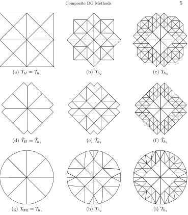
As an example, we consider the situation when Ω is a circular domain in R2,
with center at the origin and radius 3/4. The sequence of reference grids {Tˆhi}
` i=1,
generated by Algorithm 3.1, in the case when`= 3, are depicted in Figures 3.1(a)–(c). We recall that the reference meshes{Tˆhi}
`
i=1 are nested, cf. above. Formally, we
write this as follows: given ˆκi ∈Tˆhi, for somei, where 2≤i≤`, the father element ˆ
κi−1∈Tˆhi−1 such that ˆκi⊂ˆκi−1is given by the mapping
Fii−1(ˆκi) = ˆκi−1.
Thereby, the mapping
Fi`=Fii+1◦Fii+2+1◦. . .◦F``−1,
provides the link between the father elements on the reference mesh ˆThi,i= 1, . . . , `− 1, with its children on the finest reference mesh ˆTh`. More precisely, given an element ˆ
κ`∈Tˆh`, the father element ˆκi ∈Tˆhi,i= 1, . . . , `−1, which satisfies ˆκ`⊂κˆi is given by:
F`i(ˆκ`) = ˆκi.
We now proceed to define the sequence of logical and physical meshes ˜Thi andThi,
i= 1, . . . , `, respectively. To this end, we write ˆNi to denote the set of nodal (mesh)
points which define the reference mesh ˆThi, i = 1, . . . , `, respectively. The finest physical meshTh` is defined from the reference mesh ˆTh` by moving grid points ˆx∈Nˆ` of ˆTh` which are close to the boundary∂Ω, i.e., points which satisfy dist(ˆx, ∂Ω)hˆκ, for example. During this process some elements of the reference mesh ˆTh` may end up lying completely outside the computational domain; in this case, they are removed from the physical meshTh`. More precisely, the process of moving nodes ˆx∈Nˆ`onto the boundary naturally defines the bijective mapping
Φ : ˆN`→ N`,
whereN` denotes the set of mapped vertex points.
With this construction, the mapping Φ can be employed to map an element ˆ
κ∈Tˆh` to a so–called physical element κ. To simplify notation, we simply refer to this mapping as Φ as well; thereby, we write
(a) ˆTH= ˆTh1 (b) ˆTh2 (c) ˆTh3
(d) ˜TH = ˜Th1 (e) ˜Th2 (f) ˜Th3
[image:5.612.83.452.73.495.2](g)TCFE=Th1 (h)Th2 (i)Th3
Fig. 3.1. Hierarchy of meshes: (a)–(c) Reference meshes; (d)–(f ) Logical Meshes; (g)–(i) Corresponding physical meshes.
In this setting, Φ is bijective relative to the elements which are not removed from the mesh under refinement. During the process of moving nodes onto the boundary∂Ω, we noted that some elements in the reference mesh ˆTh` may be removed. With this in mind we define the finest logical mesh T˜h` to be equal to the set of elements in the reference mesh ˆTh` which are needed to construct the finest physical meshTh`. Thereby, ˜Th` ⊆ Tˆh`; indeed, in the case when Φ ≡ I (the identity operator), then clearly ˜Th` = ˆTh`. Given that any element ˜κ∈T˜h` also satisfies ˜κ∈Tˆh`, we note that
Φ(˜κ) =κ,
for someκ∈ Th`.
With this notation the physical fine meshTh` may be defined as follows:
The newly created finest physical meshTh` is a standardboundary conforming mesh upon which standard finite element/finite volume methods may be applied. In the current context, we assume that the geometry is complicated in the sense that Th` is too fine to undertake computations. Instead, we wish to only use Th` to create a coarse composite finite element meshTCFE upon which numerical simulations will be performed.
With this construction, we may now naturally create a hierarchy of logical and physical meshes {T˜hi}
`
i=1 and {Thi}
`
i=1, respectively, by simply coarsening ˜Th` and Th`, respectively. In order to ensure that these meshes are nested, the element do-mains within these meshes may consist of general polygons; this is in contrast to the construction outlined in [11] where sequences of non-nested meshes consisting of standard element types are defined. To this end, we write
˜
Thi ={˜κ: ˜κ=∪˜κ`, ˜κ`∈T˜h`, which share a common parent from mesh leveli, i.e., F`i(˜κ`) is the same for all members of this set},
Thi ={κ:κ=∪κ`, κ`∈ Th`, which share a common parent from mesh leveli, i.e., F`i(Φ−1(κ`)) is the same for all members of this set},
i = 1, . . . , `−1. Returning to the above example, when Ω is a circular domain in
R2, the sequence of logical and physical grids {T˜hi}
`
i=1 and {Thi}
`
i=1, respectively,
in the case when ` = 3, are depicted in Figures 3.1(d)–(f) and Figures 3.1(g)–(i), respectively. We refer to the coarsest level physical mesh Th1 to as the composite finite element mesh; in particular, we denote this byTCFE, i.e.,TCFE=Th1.
With this notation the mapping Φ may be employed to transform an element
κ∈ TCFEto the corresponding element ˜κ∈ Th1; here, we denote the restriction of Φ to
κby Φκsuch that Φκ(˜κ) =κ. Since only nodes close to the boundary are moved, we
assume that the element mapping Φκ defines the shape ofκ, without any significant
rescaling. With this in mind, we assume that the element mapping Φκis close to the
identity in the following sense: the Jacobi matrixJΦκ of Φκ satisfies
C1−1≤ kdetJΦκkL∞(κ)≤C1, kJ −>
Φκ kL∞(κ)≤C2, kJ −>
Φκ kL∞(∂κ)≤C3 (3.1) for all κin TCFE uniformly throughout the mesh for some positive constants C1, C2,
and C3. This will be important as our error estimates will be expressed in terms of
Sobolev norms over the element domains ˜κ.
3.2. Finite element spaces. Corresponding to the meshes {Thi}
`
i=1, we
de-fine the corresponding sequence of discontinuous Galerkin (DG) finite element spaces
V(Thi, p),i= 1, . . . , `, respectively, consisting of piecewise discontinuous polynomials of degree p. For simplicity of presentation, we first assume that the polynomial de-gree is uniformly distributed over the meshTh`; the extension to variable polynomial degrees follows in a natural fashion, cf. below. With this in mind, we write
V(Thi, p) ={u∈L2(Ω) :u|κ∈ Pp(κ)∀κ∈ Thi},
i = 1, . . . , `, where Pp(κ) denotes the set of polynomials of degree at most p ≥ 1
defined over the general polygonκ.
With this construction, noting that the meshes {Thi}
`
i=1 are nested, we deduce
that
The classical prolongation (injection) operator fromV(Thi, p) toV(Thi+1, p), 1≤i≤
`−1 is denoted by
Pii+1:V(Thi, p)→V(Thi+1, p), i= 1, . . . , `−1.
Thereby, we may define the prolongation operator from V(Thi, p) to V(Th`, p), 1≤
i≤`−1, by
Pi=P``−1P
`−1
`−2. . . P
i+1
i .
With this notation, we may writeV(Thi, p), 1≤i≤`−1, in the following alternative form
V(Thi, p) ={u∈L2(Ω) :u=P
>
i φ, φ∈V(Th`, p)}, (3.2) where the restriction operatorPi> is defined as the transpose ofPi.
Remark 3.5. The use of the prolongation operatorPi within the definition of the
finite element spacesV(Thi, p),i= 1, . . . , `, given in (3.2) allows for the introduction
of different spaces, depending on the specific choice of Pi. Indeed, here the finite element spaces are constructed in such a manner that on each (composite) element
κ∈ Thi,i= 1, . . . , `, a the restriction of a functionv∈V(Thi, p)toκis a polynomial
of degree p. This is in contrast to the construction considered in [11]; indeed, [11] employs basis functions which are piecewise polynomials on each composite element domain. Note also, that [11] employs finite element spaces consisting of continuous, rather than discontinuous, piecewise polynomials.
We now refer to V(Th1, p) as the composite finite element space V(TCFE, p), i.e.,
V(TCFE, p) =V(Th1, p). The use of a variable polynomial degree on each composite
element κ ∈ TCFE may now be admitted in a natural fashion. Indeed, writing p to denote the composite polynomial degree vector, such thatp|κ=pκ, we define the
corresponding composite finite element spaceV(TCFE,p). In this setting, it is implicitly assumed that the children of the elementκ∈ TCFEall have the same polynomial degree
pκ.
4. Composite discontinuous Galerkin finite element method. In this sec-tion, we introduce thehp-version of the (symmetric) interior penalty DGCFEM for the numerical approximation of (2.1)–(2.2). To this end, we first introduce the following notation.
We denote by FI
CFE the set of all interior faces of the partition TCFE of Ω, and by FB
CFE the set of all boundary faces of TCFE. Furthermore, we define F =FCFEI ∪ FCFEB . The boundary∂κof an elementκand the sets∂κ\∂Ω and∂κ∩∂Ω will be identified in a natural way with the corresponding subsets ofF. Letκ+andκ−be two adjacent elements of TCFE, and x an arbitrary point on the interior face F ∈ FCFEI given by
F =∂κ+∩∂κ−. Furthermore, let v and q be scalar- and vector-valued functions, respectively, that are smooth inside each element κ±. By (v±,q±), we denote the traces of (v,q) on F taken from within the interior of κ±, respectively. Then, the averages ofvandqat x∈F are given by
{{v}}= 1 2(v
++v−), {{q}}= 1 2(q
++q−),
respectively, where we denote bynκ± the unit outward normal vector of∂κ±, respec-tively. On a boundary faceF ∈ FB
CFE, we set{{v}}=v,{{q}}=q, and [[v]] =vn, withn denoting the unit outward normal vector on the boundary∂Ω.
With this notation, we make the following key assumptions: (A1) For all elements κ∈ TCFE, we define
Cκ= card
F ∈ FCFEI ∪ FCFEB :F ⊂∂κ .
In the following we assume that there exists a positive constantCF such that
max
κ∈TCFE
Cκ≤CF,
uniformly with respect to the mesh size. (A2) Inverse inequality. Given a faceF ∈ FI
CFE∪ F
B
CFEof an elementκ∈ TCFE, there exists a positive constant Cinv, independent of the local mesh size and local
polynomial order, such that
k∇vk2
L2(F)≤Cinv p2κ
hF
k∇vk2
L2(κ)
for allv∈V(TCFE,p), wherehF is arepresentativelength scale associated to
the faceF ⊂∂κ.
(A3) We assume that the polynomial degree vectorpis of bounded local variation, that is, there is a constantρ≥1 such that
ρ−1≤pκ/pκ0 ≤ρ,
wheneverκandκ0 share a common face ((d−1)–dimensional facet).
Remark 4.1. We remark that in the case whenκis a ‘standard’ (isotropic)
ele-ment in the sense thatκ= ˆκ∈TˆH, for example, the inverse inequality stated in
As-sumption (A2) immediately follows from [9, 4], for example, withhF =hκ. Moreover, [9] also considers the case when the underlying mesh consists of anisotropic elements; loosely speaking, in this latter setting, hF must be chosen to be the dimension of the elementκ in the orthogonal direction to the faceF under consideration. For general composite elements, which intersect the boundary of the computational domain, the above inverse inequality is expected to hold with hF ≈h`, whereh`≈hκ/2`−1.
With this notation, we consider the (symmetric) interior penalty DGCFEM for the numerical approximation of (2.1)–(2.2): finduh∈V(TCFE,p) such that
BDG(uh, v) =Fh(v) (4.1)
for allv∈V(TCFE,p), where
BDG(u, v) =
X
κ∈TCFE
Z
κ
∇u· ∇v dx− X
F∈FI
CFE∪FCFEB
Z
F
{{∇hv}} ·[[u]] +{{∇hu}} ·[[v]]ds
+ X
F∈FI
CFE∪F
B
CFE
Z
F
σ[[u]]·[[v]]ds,
Fh(v) =
Z
Here, ∇h denotes the elementwise gradient operator. Furthermore, the function σ∈
L∞(FI
CFE∪ F
B
CFE) is the discontinuity stabilization function that is chosen as follows: we define the functionp∈L∞(FI
CFE∪ F
B
CFE) by
p(x) :=
(
max(pκ, pκ0), x∈F ∈ FI
CFE, F =∂κ∩∂κ
0,
pκ, x∈F ∈ FCFEB , F ∈∂κ∩∂Ω,
and set
σ|F =γp2h−F1, (4.2)
with a parameterγ >0 that is independent ofhF andp.
5. Stability analysis. Before embarking on the error analysis of thehp–version DGCFEM (4.1), we first derive some preliminary results. Let us first introduce the DG–norm||| · |||DG by
|||v|||2DG= X
κ∈TCFE
k∇vk2L2(κ)+ X
F∈FI
CFE∪F
B
CFE
kσ1/2[[v]]k2L2(F). (5.1)
For a given faceF ∈ FI
CFE∪ FCFEB , such that F ⊂∂κfor some κ∈ TCFE, we write ˜
F to denote the respective face of the mapped element ˜κ based on employing the element mapping Φκ. More precisely, we write ˜F = Φ−κ1(F). Further, we definemF
and mF˜ to denote the (d−1)–dimensional measure (volume) of the faces F and ˜F,
respectively. In view of (3.1), we note that there exists a positive constant C4, such
that
C4−1mF˜ ≤mF ≤C4mF˜ (5.2)
for every face F ∈ FI
CFE∪ FCFEB . Moreover, the surface JacobianSF,F˜ arising in the
transformation of the faceF to ˜F may be uniformly bounded in the following manner
kSF,F˜kL∞( ˜F)≤C5 (5.3)
for all facesF ∈ FI
CFE∪ FCFEB , whereC5is a positive constant.
Lemma 5.1. Withσdefined as in (4.2), there exists a positive constantC, which
depends only on the constantsCF andCinv, cf. Assumptions (A1) , (A2) and (A3) above, respectively, such that
BDG(v, v)≥C|||v|||DG2 ∀v∈V(TCFE,p), (5.4)
provided that the (positive) constant γ arising in the definition of the discontinuity penalization parameterσ is chosen sufficiently large.
Proof. Forv∈V(TCFE,p), we note that
BDG(v, v) =
X
κ∈TCFE
k∇vk2
L2(κ)−2
X
F∈FI
CFE∪FCFEB
Z
F
{{∇v}} ·[[v]] ds+ X
F∈FI
CFE∪FCFEB
kσ1/2[[v]]k2
L2(F),
≡I + II + III. (5.5)
In order to bound term II, we first note that forF∈ FI
CFE, we have that
Z
F
{{∇v}} ·[[v]] ds≤ kσ−1/2{{∇v}}kL2(F)kσ
1/2[[v]]k L2(F)
≤ 1 2
kσ−1/2∇v+kL2(F)+kσ −1/2
∇v−kL2(F)
kσ1/2[[v]]kL2(F)
≤kσ−1/2∇v+k2L2(F)+kσ−1/2∇v−k2L2(F)+ 1 8kσ
1/2[[v
here, we have employed the Cauchy–Schwarz inequality, together with the arithmetic– geometric mean inequality. Employing the inverse inequality stated in Assump-tion (A2), together with (A3), we deduce that
Z
F
{{∇v}} ·[[v]] ds≤Cinv p2
κ+
hF
kσ−1/2∇vk2
L2(κ+)+
p2
κ−
hF
kσ−1/2∇vk2
L2(κ−)
+1 8kσ
1/2[[v]]k2
L2(F)
≤ Cinvρ
2
γ
k∇vk2L2(κ+)+k∇vk
2
L2(κ−)
+ 1 8kσ
1/2[[v
]]k2L2(F),(5.6)
where we have used the definition of the interior penalty parameterσ, cf. (4.2). In an analogous fashion, forF∈ FB
CFE, we have that
Z
F
{{∇v}} ·[[v]] ds≤Cinv
γ k∇vk 2
L2(κ+)+
1 4kσ
1/2
[[v]]k2L2(F). (5.7)
Thereby, exploiting Assumption (A1) above, inserting (5.6) and (5.7) into (5.5) gives
BDG(v, v) =
1−CinvCFρ
2
γ
X
κ∈TCFE
k∇vk2
L2(κ)+
1− 1 4
X
F∈FI
CFE∪FCFEB
kσ1/2[[v]]k2
L2(F).
Thereby, the bilinear formBDG(·,·) is coercive overV(TCFE,p)×V(TCFE,p), assuming that >1/4 andγ > CinvCFρ2.
6. Approximation results. In this section we develop the approximation re-sults needed for the forthcominga priorierror estimation developed in Section 7. To this end, givenκ∈ TCFE, we write ˜κ∈T˜h1 to denote the corresponding element from
the logical mesh ˜Th1 which satisfies Φ(˜κ) =κ. Moreover, we write ˆκ∈Tˆh1 to denote
the element in the reference mesh ˆTh1 such that ˜κ⊆κˆ.
With this notation, we now recall the following approximation result.
Lemma 6.1. Suppose thatˆκ∈Tˆh1 is a d–simplex ord–parallelepiped of diameter
hˆκ. Suppose further that v|κˆ∈Hkκˆ(ˆκ),kκˆ ≥0, for ˆκ∈Tˆh1. Then, there exists Πˆpv inPpˆκ(ˆκ),pκˆ= 1,2, . . . , such that for0≤m≤kκˆ,
kv−ΠˆpvkHm(ˆκ)≤C
hsˆκ−m
ˆ
κ
pkκˆ−q
ˆ
κ
kvkHkˆκ(ˆκ),
where 1≤sˆκ ≤min{pκˆ+ 1, kˆκ}, pκˆ ≥1, for κˆ ∈Tˆh1, and C is a positive constant, independent ofv and the discretisation parameters.
Proof. For the proof, see Lemma 4.5 in [5] ford= 2; whend >2 the argument is completely analogous.
Given the operator ˆΠp defined in Lemma 6.1, we define the projection operators
˜
Πp and Πp on ˜κandκ, respectively, by the relations
˜
Πp˜v= ˆΠp(Ev˜)|˜κ, Πpv= ( ˜Πp(v◦Φ))◦Φ−1,
Lemma 6.2. Given κ∈ TCFE, letF ⊂∂κ denote one of its faces. For a function
v∈Hkκ(κ), the following bounds hold
|v−Πpv|Hm(κ)≤C
hsκ−m
κ
pkκ−m
κ
kE˜vkHkκ(ˆκ), (6.1)
|v−Πpv|Hm(F)≤C 1
h1F/2
hsκ−m
κ
pkκ−m−1/2
κ
kE˜vkHkκ(ˆκ), (6.2)
where 0≤m≤kκ,1 ≤sκ≤min{pκ+ 1, kκ}, pκ ≥1, andC is a positive constant, independent ofv and the discretisation parameters.
Proof. The proof is based on exploiting a scaling argument together with (3.1) and Lemma 6.1. To this end, we have
|v−Πpv|2Hm(κ)≤ kdetJΦκkL∞(κ)kJ −>
Φκ k
2m L∞(κ)|˜v−
˜
Πpv˜|2Hm(˜κ) ≤C1(C2)2m|Ev˜−Πˆp(Ev˜)|2Hm(ˆκ)
≤Ch 2(sκ−m)
κ
p2(kκ−m)
κ
kEv˜k2
Hkκ(ˆκ), (6.3)
which gives (6.1). To prove (6.2), we first recall the multiplicative trace inequality
kvk2L2(F)≤C(k∇vkL2(κ)kvkL2(κ)+h −1
F kvk
2
L2(κ)), (6.4)
where C is a positive independent of the meshsize. We remark, cf. Remark 4.1, that hF appears in (6.4) rather than hκ due to the general shape of the element κ.
Employing (6.4), together with (3.1), (5.3), (5.2) and (6.1) we immediately deduce (6.2).
7. A priori error analysis. In this section we derive ana priorierror bound for the interior penalty DGCFEM introduced in Section 4. To this end, we decompose the global erroru−uhas
u−uh= (u−Πpu) + (Πpu−uh)≡η+ξ , (7.1)
where Πp denotes the projection operator introduced in Section 6. With these
defini-tions we have the following result.
Lemma 7.1. Foru∈ H3/2+(Ω), >0, the functions ξ andη defined by (7.1)
satisfy the following inequality
|||ξ|||DG≤C|||η|||∗DG,
where
|||η|||∗DG=
X
κ∈TCFE
k∇ηk2
L2(κ)+ X
F∈FI
CFE∪F
B
CFE
kσ−1/2{{∇η}}k2
L2(F)+kσ
1/2[[η]]k2
L2(F)
1/2
andC is a positive constant that depends only on the dimensiond.
Proof. This result follows from application of the Galerkin orthogonality of the DGCFEM, together with the inverse inequality in Assumption (A2); for details, see [12, 19].
Theorem 7.2. Let Ω ⊂ Rd be a bounded polyhedral domain, and let TCFE = {κ} be a subdivision of Ω as outlined in Section 3.1, where κhas diameter hκ. Let
uh ∈V(TCFE, p)be the composite discontinuous Galerkin approximation to udefined
by (4.1)and suppose that u|κ ∈Hkκ(κ)for each κ∈ TCFE for integers kκ≥1. Then, the following error bound holds
|||u−uh|||2DG≤C
X
κ∈TCFE
h2sκ
κ
h2
F
1
p2kκ−3
κ
kEu˜k2
Hkκ(ˆκ),
for any integers sκ, 1 ≤ sκ ≤min(pκ+ 1, kκ), and pκ ≥ 1. Here, C is a positive constant that depends only on the dimensiondand the shape-regularity of TˆH.
Proof. Decomposing the erroru−uh as in (7.1), and exploiting Lemma 7.1, we
deduce that
|||u−uh|||DG≤ |||η|||DG+C|||η|||∗DG≤(1 +C)|||η|||
∗
DG. (7.2)
Employing Lemma 6.2, together with the definition of the interior penalty parameter (4.2), we deduce that
|||η|||∗DG≤C "
X
κ∈TCFE
h2(sκ−1)
κ
p2(kκ−1)
κ
+h
2(sκ−1)
κ
p2kκ−1
κ
+h
2sκ
κ
h2
F
1
p2kκ−3
κ
!
kEu˜k2
Hkκ(ˆκ) #1/2
,(7.3)
whereCis a positive constant, which is independent of the mesh parameters. Inserting (7.3) into (7.2) gives the statement of the Theorem.
Remark 7.3. We note that since the fine mesh Th` is fixed, we have that
hF ≥
hκ
2`−1.
Thereby, the a priori error bound derived in Theorem 7.2 may be rewritten in the following form:
|||u−uh|||2DG≤C
0 X
κ∈TCFE
h2(sκ−1)
κ
p2kκ−3
κ
kEu˜k2
Hkκ(ˆκ),
where C0 = C2`−1. Moreover, for uniform orders pκ = p ≥ 1, sκ = s, 2 ≤ s ≤
min(p+ 1, k),k≥1, andh= maxκ∈TCFEhκ, we get the bound
|||u−uh|||DG≤C
hs−1 pk−3/2ku˜k
2
Hk(Ω);
here, we have employed Theorem 2.1. This bound is optimal inh, suboptimal inpby
p1/2, and coincides with estimates derived in [12] and [15] for so-called standard DG methods.
8. Implementation. In this section we discuss several aspects concerning the implementation of the DGCFEM. To this end, we first write
ACFExCFE=fCFE
to denote the linear system of equations stemming from the discretization of (2.1)– (2.2), based on employing the DGCFEM (4.1), which utilizes the CFE finite element spaceV(TCFE,p). Similarly, we write
to denote the linear system of equations which arise from the standardDGFEM dis-cretization of problem (2.1)–(2.2) based on employing the (standard) finite element space V(Th`, p) consisting of discontinuous piecewise polynomials of degree p. The entries of the matrixACFE and those of the vectorfCFEfor the CFE method are com-puted in a different manner to the those for the standard DG method. Indeed, the sparsity of the matrixACFEreflects the topology of the meshTCFE; thereby, the actual values of the entries in both the matrixACFEand vector fCFE are computed based on aggregating the appropriate entries of Ah` and fh`, respectively. The construction of the CFE space, as described in Section 3, implies that even when the mesh TCFE contains just a small number of elements, the supports of the corresponding compos-ite fincompos-ite element basis functionsφCFEwhich belong to the spaceV(TCFE,p) accurately reflect the complexity of the geometry of the underlying computational domain Ω
There are two key aspects related to the construction of the matrix and right-hand side vectorACFEandfCFE, respectively. Firstly, any basis functionφCFEwhich belongs to the space V(TCFE,p) also belongs to the polynomial space Pp(κCFE), where κCFE is the composite finite element domain over whichφCFE is defined. Thereby, in case whenp= 1 andd= 2, there are three basis functions φCFE,i, i= 1, . . . ,3, associated
to the elementκCFE; here, the indexi denotes a local ordering of the basis functions related toκCFE. Secondly, any basis functionφCFE,i,i= 1, . . . ,dim(V(TCFE,p)), wherei now denotes the global ordering of the basis functions, can be constructed as a linear combination of the basis functionsφh`,j ofV(Th`, p), i.e.,
φCFE,i:=
X
j=1,...,dim(V(Th`,p))
αi,jφh`,j , (8.1)
where αi,j are real coefficients which determine how the CFE space V(TCFE,p) is constructed from the standard finite element space V(Th`, p). This representation follows immediately, since it is assumed the meshes are nested and that all the children elements of a CFE elementκCFEhave the same polynomial degree asκCFE; indeed, we have thatV(TCFE,p)⊂V(Th`, p). Writing Λ to denote the set of all coefficients αi,j, we deduce from (8.1) that]Λ = dim(V(Th`, p))×dim(V(TCFE,p)). A straightforward consequence of (8.1) is that any entryACFE[i, r] of the matrixACFE is simply a linear combination of the entries ofAh`; indeed, we note that
ACFE[i, j] =BDG(φCFE,i, φCFE,j) :=
X
m,n=1,...,dim(V(Th`,p))
αi,mαj,nBDG(φh`,m, φh`,n)
= X
m,n=1,...,dim(V(Th`,p))
αi,mαj,nAh`[m, n]. (8.2)
Similarly, the entries present in the vectorfCFEmay be defined in an analogous fashion:
fCFE[i] =Fh(φCFE,i) :=
X
j=1,...,dim(V(Th`,p))
αi,jFh(φh`,j)
= X
j=1,...,dim(V(Th`,p))
αi,jfh`[j]. (8.3)
Remark 8.1. From (8.2) and (8.3) it is clear that in order to construct ACFE
and fCFE, it is not necessary to store Ah` and fh`, which would potentially require a
fCFE from the entries ofAh` andfh`, respectively, using the above linear combinations
determined by the coefficients αi,j. In this way, the amount of memory required to construct the linear system of equations stemming from the CFE method is essentially just the memory needed to storeACFE andfCFE (which are generally small, compared
toAh` andfh`) and the coefficientsαi,j. However, the CPU time needed to construct
the CFE linear system is clearly dependent on the dimension of the underlying finite element spaceV(Th`, p).
As already stated above, the role of the coefficientsαi,j is to provide information
concerning how the basis functions φCFE,i present in the coarse space V(TCFE,p) are defined in terms of the basis functions defined on the finer spaceV(Th`, p). We remark that this construction is element-wise in the sense that for each elementκ∈V(Th`, p), there is a subset of coefficients Λκ⊂Λ, such that the corresponding linear combination
of the basis functions defined onκ, reconstruct the restriction of the basis functions defined on the father element κCFE to κ. Repeating this process for all children κ of κCFE, we are able to entirely reconstruct the basis functions of the coarse space defined on κCFE. Since it is assumed that the same order of polynomialsp are used on both κ and its father, we have that]Λκ =n2κ, wherenκ denotes the dimension
of the local polynomial space on elementκ; i.e.,nκ=pκ(pκ+ 1)/2 in the case when
triangular elements are used in two–dimensions, for example. An interesting property of these coefficients αi,j is that they are completely independent of the underlying
PDE problem at hand, but only depend on the two finite element spaces V(TCFE,p) and V(Th`, p). We write φCFE,κCFE,i, i = 1, . . . ,dim(Pp(κCFE)), to denote the basis
functions defined over element κCFE∈ TCFE; similarly, φh`,κ,j, j = 1, . . . ,dim(Pp(κ)), denotes the corresponding set of basis functions associated with element κ ∈ Th`. Given thatκCFE∈ TCFE is defined as the union of their child elements present inTh`, the intersection between the support of a basis function φCFE,κCFE,i defined overκCFE
and a basis functionφh`,κ,j defined onκ∈ Th` is zero unless the elementκis a child of
κCFE; if this latter condition is not satisfied, then clearly, the corresponding coefficients present inαi,jbe identically equal to zero. This observation dramatically reduces the
number of coefficients that need to be computed; indeed, we may characterize the coefficients that may be non-zero as follows
Λ0:= [
κ∈Thl
Λκ , Λ0⊂Λ ,
which implies that]Λ0=Pκ∈T
hln
2
κ< ]Λ.
The most general way to compute the coefficients Λ0 is by solving a family of
square linear systemsR. The family Rcan be split in subfamilies Rκ, one for each
element κ∈ Th`. All the linear systems in the same subfamilyRκ are characterized to have the same matrix, but a different right-hand side. This can be exploited, for example, when an LU decomposition is used to solve all the linear systems in the family, since even if there are as many linear systems to solve as the number of elements in Th` times the dimension of the space V(TCFE,p), only as many LU decompositions as the number of elements in Th` are needed. Denoting byκCFE the father of an elementκ, and by{αi,j}the set of coefficients corresponding to the basis
functions of the two elements, we have that the linear systems in the subfamily ofκ
have the form
Cκακ,i=φκ,i ,
basis function φCFE,κCFE,i on the support of κ, the matrix Cκ is the same for any
φCFE,κCFE,i and φκ,i depends on the restriction of φCFE,κCFE,i to κ. The dimension of
the linear systems in the subfamily is equal to the number of basis functions of the element κ, which is the same as the number of basis functions of its father element
κCFE, due to the constraint on the choice of polynomial orders we imposed between the two meshes.
In order to define the matrices Cκ and vectors φκ,i, we need do define a set
of points Qκ,p, for each element κ, whose cardinality depends on the order of the
approximating polynomialpon the element. As an example, letκref be the reference triangle with vertices (0,0), (1,0) and (0,1); moreover letQs, with s∈ R+, be the
set of all pointsq in the real plane such thatq:= (nse1, mse2), withn, m∈Nand e1,e2 is the canonical basis ofR2. Then the setQκ,p is defined as:
Qκ,p:=Aκ(Q1/p∩κref),
where Aκ is the affine transformation which maps κref into κ. The points present
in Qκ,p, define where the basis functions φCFE,κCFE,i, φh`,κ,j are evaluated in order to assemble the matrices Cκ and the vectors φκ. Indeed, for any κand any φCFE,κCFE,i
the vectorφκ is given by
φκ,i[j] :=φCFE,κCFE,i(qj) ∀qj ∈ Qκ,p.
Similarly, for anyκ, the matrixCκ is defined as
Cκ[r, j]; =φh`,κ,r(qj) ∀qj∈ Qκ,p ∀φh`,κ,r .
The computation of the solutions of all these linear systems can be quite expen-sive; however, this process may be undertaken in a more efficient manner. To this end, suppose for the moment that both finite element spacesV(TCFE,p) andV(Th`, p) employ a set of nodal Lagrange basis function on each element. Then, it follows straightforwardly, from the properties of the nodal basis functions and the definitions of the setsQκ,p, that all matricesCκ reduce to the identity matrix. Thereby, in this
case, we conclude that
ακ,i≡φκ,i ;
in this case the computation of the coefficients in Λ0, simply requires the evaluation of
the basis functionsφCFE,iat the nodes determined by the setsQκ,p. With this
obser-vation, more general modal bases may be considered, with only a small computational overhead. Indeed, suppose that for anyp,Bpis the matrix that transforms the nodal
polynomial basis for Pp into an alternative basis which spans the same polynomial
space, such as a modal basis, for example. Since these matricesBpare invariant under
affine transformations, they can be computed just for the reference element in advance and stored. Now, if for the example when modal basis functions are employed within both finite element spacesV(TCFE,p) and V(Th`, p), then the components of the sys-tems ˜Cκα˜κ,i= ˜φκ,i for the modal basis functions are equivalent to the components
of the systems for the nodal basis functions in the following manner:
Cκ≡B−p1C˜κBp, φκ,i≡B−p1φ˜κ,i ,
i.e., ˜ακ,i := Bpακ,i. This approach is extremely cheap, since it does not require
the inversion of a linear system of equations; indeed, the matrices Bp can be all
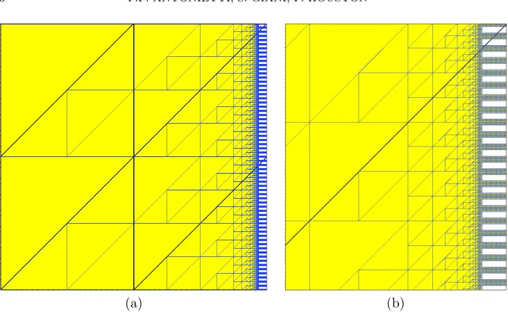
(a) (b)
Fig. 9.1. Example 1: (a) Initial composite finite element mesh. The colour blue denotes elements present in the fine level mesh (which consists of 20160 triangular elements); elements plotted in black form the coarse level mesh (containing 8 elements); finally, the domainΩis shown in yellow. (b) Zoom of (a).
9. Numerical experiments. In this section we present a series of computa-tional examples to numerically investigate the asymptotic convergence behaviour of the proposed DGCFEM for problems where the underlying computational domain contains micro-structures. Throughout this section the DGCFEM solutionuhdefined
by (4.1) is computed with the constant γ appearing in the interior penalty param-eter σ defined by (4.2) equal to 10. All the numerical examples presented in this section have been computed using the AptoFEM package (www.aptofem.com); here, the resulting system of linear equations is solved based on employing the Multifrontal Massively Parallel Solver (MUMPS), see [1, 2, 3].
9.1. Two–dimensional domain with a complicated boundary. In this first example, we consider a computational domain with a complicated boundary; to this end, we let Ω be the unit square in two–dimensions, where a series of tiny ‘finger– like’ cuts have been removed from the right-hand boundary, i.e., where x = 1, 0≤
y ≤ 1. More precisely, the right-hand side boundary of the domain possesses 64 equidistributed tiny ‘gaps’; cf. Figure 9.1. In this example, we select the right-hand side forcing functionf and appropriate inhomogeneous boundary conditionu=g on
∂Ω, so that the analytical solution to (2.1)–(2.2) is given byu= tanh(2x).
In order to compute the numerical approximation to (2.1)–(2.2) using the DGCFEM defined in (4.1), we first construct a sequence of meshes based on employing Algo-rithm 3.1. To this end, the coarsest mesh reference mesh ˆTHis selected to be a uniform
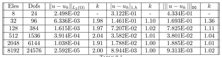
Eles Dofs ku−uhkL2(Ω) k |u−uh|1,h k |||u−uh|||DG k
8 24 2.498E-02 - 3.122E-01 - 4.334E-01
-32 96 6.336E-03 1.98 1.461E-01 1.10 1.693E-01 1.36
128 384 1.615E-03 1.97 7.207E-02 1.02 7.825E-02 1.11
512 1536 3.914E-04 2.04 3.582E-02 1.01 3.801E-02 1.04
2048 6144 1.038E-04 1.91 1.788E-02 1.00 1.885E-02 1.01
[image:17.612.72.441.92.187.2]8192 24576 2.592E-05 2.00 8.944E-03 1.00 9.313E-03 1.02
Table 9.1
Example 1: Convergence of the DGCFEM on a sequence of uniform triangular composite ele-ments withp= 1.
Eles Dofs ku−uhkL2(Ω) k |u−uh|1,h k |||u−uh|||DG k
8 48 4.744E-03 - 4.998E-02 - 7.600E-02
-32 192 5.870E-04 3.01 1.553E-02 1.69 2.038E-02 1.90
128 768 7.512E-05 2.97 3.924E-03 1.98 4.754E-03 2.10
512 3072 1.228E-05 2.61 9.881E-04 1.99 1.119E-03 2.09
2048 12288 1.108E-06 3.47 2.446E-04 2.01 2.717E-04 2.04
8192 49152 1.398E-07 2.99 6.124E-05 2.00 6.598E-05 2.04
Table 9.2
Example 1: Convergence of the DGCFEM on a sequence of uniform triangular composite ele-ments withp= 2.
be exactly triangulated using Algorithm 3.1, without the need to move any nodal points in the finest reference mesh. Thereby, in this setting, the respective hierarchy of logical and physical meshes are both identical.
We now investigate the asymptotic convergence of the proposed DGCFEM on a sequence of successively finer uniform triangular meshes, starting withTCFEconsisting of 8 composite elemental domains, for p= 1,2; see Tables 9.1 & 9.2, respectively. In each case we show the number of elements (Eles) and number of degrees of freedom (Dofs) in the composite finite element spaceV(TCFE,p), theL2(Ω), the brokenH1 (Ω)-semi-norm (denoted by|·|1,h) and the DG–norm of the erroru−uh, together with their
respective rates of convergence, denoted bykin each case. We remark that none of the (composite) finite element meshes employed here are fine enough to exactly represent the computational domain Ω.
From Tables 9.1 & 9.2, we observe that both theL2(Ω) norm and brokenH1(Ω) seminorm of the error converge at the expected optimal rate, even in the presence of such micro-structure present in the boundary of the computational domain Ω. More precisely, we observe that ku−uhkL2(Ω) and |u−uh|1,h converge to zero like
O(hp+1) and O(hp), respectively, for each fixed p, as h tends to zero. In terms
of the convergence of the DGCFEM with respect to the DG–norm, we observe the convergence rateO(hp), ashtends to zero, for each fixedp; this corresponds to the
expected rate of convergence of the so-calledstandardDGFEM, cf. [4], for example, in the absence of micro-structures. The observed rate of convergence of the DGCFEM with respect to the DG–norm is in accordance with Theorem 7.2, since most elements
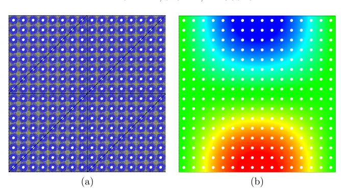
(a) (b)
Fig. 9.2. Example 2: (a) Initial composite finite element mesh. The colour blue denotes elements present in the fine level mesh (which consists of 85500 triangular elements); elements plotted in black form the coarse level mesh (containing 8 elements); finally, the domainΩis shown in yellow. (b) Analytical solution.
9.2. Two–dimensional domain with micro-structures. In this second ex-ample, we consider the case when the computational domain Ω contains a large num-ber of small geometric features. To this end, we set Ω to be the unit square (0,1)2in
two-dimensions, which has had a series of uniformly spaced circular holes removed; here, we consider the case where 256 small circular holes are removed from (0,1)2, see Figure 9.2(a). In this example, we select the right-hand side forcing function f and appropriate inhomogeneous boundary conditionu=g on∂Ω, so that the analytical solution to (2.1)–(2.2) is given byu= sin(πx) cos(πy), cf. Figure 9.2(b).
As in the previous example, we first define the coarsest reference mesh ˆTH to be a
uniform triangular mesh consisting of 8 elements. This mesh is then refined to generate a sequence of reference meshes according to Algorithm 3.1. Given that the underlying geometry cannot be exactly represented by such a sequence of refined meshes, nodes close to the boundary are moved in order to provide an accurate description of the computational domain. Thereby, in this setting the corresponding sequence of physical meshes differ from their respective logical and reference meshes. Here, the fine mesh consists of 85500 triangular elements; in particular, edges of elements present in the fine mesh which have nodes on one of the circular holes are curved using a local quadratic representation of the edge. We remark that, to avoid ‘cracks’ appearing in the finest mesh in the vicinity of the holes present in Ω when nodes are locally moved, additional refinement has been undertaken near the circular boundaries.
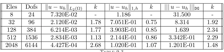
In Tables 9.3 & 9.4 we investigate the asymptotic convergence of the proposed DGCFEM on a sequence of successively finer uniform triangular meshes, starting withTCFEconsisting of 8 composite elemental domains, for p= 1,2, respectively. As in the previous example, we compute the L2(Ω), the brokenH1(Ω)-semi-norm and the DG–norm of the erroru−uh, together with their respective rates of convergence.
For this example, the rates of convergence are less consistent than those reported in the previous example. For bothp= 1 and p= 2, the quantitiesku−uhkL2(Ω) and
|u−uhk1,happear to convergence slightly sub-optimally, excluding on the last mesh,
Eles Dofs ku−uhkL2(Ω) k |u−uhk1,h k |||u−uh|||DG k
8 24 7.320E-02 - 1.186 - 31.500
-32 96 2.120E-02 1.78 7.051E-01 0.75 8.314 1.92
128 384 6.214E-03 1.77 3.903E-01 0.85 1.639 2.34
512 1536 2.834E-03 1.13 2.144E-01 0.86 3.342E-01 2.29
[image:19.612.77.437.91.175.2]2048 6144 4.427E-04 2.68 1.020E-01 1.07 1.201E-01 1.48
Table 9.3
Example 2: Convergence of the DGCFEM on a sequence of uniform triangular composite ele-ments withp= 1.
Eles Dofs ku−uhkL2(Ω) k |u−uh|1,h k |||u−uh|||DG k
8 48 1.699E-02 - 4.089E-01 - 13.447
-32 192 2.477E-03 2.78 1.078E-01 1.92 1.941 2.79
128 768 5.734E-04 2.11 3.739E-02 1.53 3.159E-01 2.62
512 3072 1.531E-04 1.91 1.288E-02 1.54 3.208E-02 3.30
2048 12288 1.088E-05 3.81 2.212E-03 2.54 2.515E-03 3.67
Table 9.4
Example 2: Convergence of the DGCFEM on a sequence of uniform triangular composite ele-ments withp= 2.
standard DGFEM; in the latter case, we simply compute the numerical solution on the unit square (0,1)2 without any holes. Here, we now observe that the accuracy and rate of convergence of the DGCFEM, which takes into account the holes present in the computational domain, is very similar to the standard DGFEM which cannot treat the micro-structures present in Ω on such coarse meshes. Indeed, this clearly illustrates that the presence holes/micro-structures in the computational domain does
notlead to a degradation in the quality of the computed solution when the DGCFEM is exploited. Finally, Tables 9.3 & 9.4 indicate that the DG-norm of the error in the DGCFEM solution converges to zero at a faster rate than we would expect for the standard DGFEM. This is in accordance with Theorem 7.2, due to the definition of
hF; indeed, as noted in Remark 4.1,hF may be selected to be equal to the element
dimension only on ‘standard’ element domains, while on composite element domains, we must selecthF to be equal to the size of the elements present in the fine mesh.
For this latter choice, hF is effectively fixed as the composite finite element mesh
is refined; thereby, the order of convergence of the DGCFEM with respect to the DG-norm may exceed the standard predicted order ofO(hp), cf. Theorem 7.2.
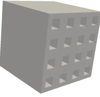
9.3. Three–dimensional domain with micro-structures. In this final ex-ample, we consider a three–dimensional problem which contains a number of holes. More precisely, we let Ω to be the unit cube (0,1)3 which has had 16 rectangular sections removed; cf. Figure 9.4. We point out that the holes only go to a depth of a half of the domain width. We select the right-hand side forcing function f and appropriate inhomogeneous boundary conditionu=g on∂Ω, so that the analytical solution to (2.1)–(2.2) is given byu= sin(πx) cos(πy) sin(πz).
Here, the coarsest mesh reference mesh ˆTH is selected to be a uniform tetrahedral
[image:19.612.73.438.219.298.2]do-101 102 10−6
10−5 10−4 10−3 10−2 10−1 100
p=1
p=2
dof1/2
L2
−Error
DGCFEM DGFEM
101 102
10−3 10−2 10−1 100
p=1
p=2
dof1/2
H
1−Error
DGCFEM DGFEM
[image:20.612.75.444.77.256.2](a) (b)
Fig. 9.3.Example 2. Comparison between the DGCFEM and the standard DGFEM (computed without any holes): (a)ku−uhkL2(Ω); (b)|u−uh|1,h.
Fig. 9.4.Computational domainΩ.
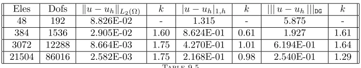
main Ω. Here, we point out that the choice of the initial mesh and the definition of Ω have been selected so that Ω may be exactly triangulated using Algorithm 3.1, with-out the need to move any nodal points in the finest reference mesh. The asymptotic convergence of the proposed DGCFEM on a sequence of successively finer uniform tetrahedral meshes, starting withTCFEconsisting of 48 composite elemental domains, forp= 1,2 is investigated Tables 9.5 & 9.6, respectively. Here, we observe that the
L2(Ω)–norm of the error converges at a slightly sub-optimal rate for p= 1, though |u−uh|1,h tends to zero at roughly the optimal rate of O(hp), for each fixed p, as
the mesh is uniformly refined. As in the previous example, the DG–norm of the error again converges to zero, as the mesh is refined, at a slightly faster rate compared to the expected rate when the standard DGFEM is employed, cf. Theorem 7.2.
[image:20.612.176.342.301.462.2]Eles Dofs ku−uhkL2(Ω) k |u−uh|1,h k |||u−uh|||DG k
48 192 8.826E-02 - 1.315 - 5.875
-384 1536 2.905E-02 1.60 8.624E-01 0.61 1.927 1.61
3072 12288 8.664E-03 1.75 4.270E-01 1.01 6.194E-01 1.64
[image:21.612.72.441.93.163.2]21504 86016 2.582E-03 1.75 2.168E-01 0.98 2.540E-01 1.29
Table 9.5
Example 3: Convergence of the DGCFEM on a sequence of uniform triangular composite ele-ments withp= 1.
Eles Dofs ku−uhkL2(Ω) k |u−uh|1,h k |||u−uh|||DG k
48 480 2.707E-02 - 5.577E-01 - 2.931
-384 3840 5.075E-03 2.42 1.770E-01 1.66 4.557E-01 2.69
3072 30720 5.983E-04 3.08 4.288E-02 2.05 6.015E-02 2.92
21504 215040 7.401E-05 3.01 1.076E-02 1.99 1.250E-02 2.27
Table 9.6
Example 3: Convergence of the DGCFEM on a sequence of uniform triangular composite ele-ments withp= 2.
approximation of PDE problems posed on complicated domains which contain local geometrical features in an efficient manner. In this article we have undertaken thea priori error analysis of the proposed DGCFEM, based on generating a hierarchy of meshes, such that the finest mesh does indeed provide an accurate representation of the underlying computational domain. The finite element spaces can then be defined in a very natural manner, based on employing appropriate prolongation operators. The approach here is to recover finite element spaces, such that on each composite element the numerical solution is a polynomial; by selecting alternative prolongation operators, cf. [11], for example, finite element basis functions which are piecewise polynomial on each composite element may also be defined. Numerical experiments highlighting the application of the proposed DGCFEM for a range of two– and three– dimensional problems have been presented. Future work will be concerned with thea posteriorierror analysis of DGCFEMs, as well as the application of DGCFEMs within two–level Schwarz–type preconditioners.
Acknowledgements. SG and PH acknowledge the financial support of the EP-SRC under the grant EP/H005498.
REFERENCES
[1] P. R. Amestoy, I. S. Duff, J. Koster, and J.-Y. L’Excellent. A fully asynchronous multifrontal solver using distributed dynamic scheduling. SIAM Journal on Matrix Analysis and Ap-plications, 23(1):15–41, 2001.
[2] P. R. Amestoy, I. S. Duff, and J.-Y. L’Excellent. Multifrontal parallel distributed symmetricand unsymmetric solvers. Comput. Methods Appl. Mech. Eng., 184:501–520, 2000.
[3] P. R. Amestoy, A. Guermouche, J.-Y. L’Excellent, and S. Pralet. Hybrid scheduling for the parallel solution of linear systems. Parallel Computing, 32(2):136–156, 2006.
[4] D.N. Arnold, F. Brezzi, B. Cockburn, and L.D. Marini. Unified analysis of discontinuous Galerkin methods for elliptic problems.SIAM J. Numer. Anal., 39:1749–1779, 2001. [5] I. Babuˇska and M. Suri. Thehp–version of the finite element method with quasiuniform meshes.
RAIRO Anal. Num´er., 21:199–238, 1987.
[image:21.612.72.445.211.278.2]stabilized Lagrange multiplier method. Comput. Methods Appl. Mech. Engrg., 199:2680– 2686, 2010.
[7] E. Burman and P. Hansbo. An interior-penalty-stabilized Lagrange multiplier method for the finite-element solution of elliptic interface problems. IMA J. Numer. Anal., 30:870–885, 2010.
[8] E. Burman and P. Hansbo. Fictitious domain finite element methods using cut elements: II. A stabilized Nitsche method.Appl. Numer. Math., 62:328–341, 2012.
[9] E.H. Georgoulis, E. Hall, and P. Houston. Discontinuous Galerkin methods for advection– diffusion–reaction problems on anisotropically refined meshes. SIAM J. Sci. Comput., 30(1):246–271, 2007.
[10] W. Hackbusch and S.A. Sauter. Composite finite elements for problems containing small geo-metric details. Part II: Implementation and numerical results. Comput. Visual Sci., 1:15– 25, 1997.
[11] W. Hackbusch and S.A. Sauter. Composite finite elements for the approximation of PDEs on domains with complicated micro-structures.Numer. Math., 75:447–472, 1997.
[12] P. Houston, C. Schwab, and E. S¨uli. Discontinuoushp-finite element methods for advection– diffusion–reactio n problems.SIAM J. Numer. Anal., 39:2133–2163, 2002.
[13] A. Johansson and M.G. Larson. A high order discontinuous Galerkin Nitsche method for elliptic problems with fictitious boundary.Submitted for publication, 2011.
[14] M. Rech, S. Sauter, and A. Smolianski. Two-scale composite finite element method for the Dirichlet problem on complicated domains. Numer. Math., 102(4):681–708, 2006. [15] B. Rivi`ere, M.F. Wheeler, and V. Girault. Improved energy estimates for interior penalty,
constrained and discontinuous Galerkin methods for elliptic problems, Part I. Comput. Geosci., 3:337–360, 1999.
[16] S. A. Sauter and R. Warnke. Extension operators and approximation on domains containing small geometric details.East-West J. Numer. Math., 7(1):61–77, 1999.
[17] G.H. Shortley and R. Weller. Numerical solution of laplaces equation.J. Appl. Phys, 9:334–348, 1938.
[18] E. M. Stein. Singular Integrals and Differentiability Properties of Functions. Princeton, Uni-versity Press, Princeton, N.J., 1970.
[19] E. S¨uli, Ch. Schwab, and P. Houston. hp–DGFEM for partial differential equations with non-negative characteristic form. In B. Cockburn, G.E. Karniadakis, and C.-W. Shu, editors,