Normal and Bootstrap Confidence Intervals in Bitterlich Sampling

(1)

ISSN Print: 2163-0429

DOI: 10.4236/ojf.2020.101005 Dec. 13, 2019 58 Open Journal of Forestry

Normal and Bootstrap Confidence Intervals in

Bitterlich Sampling

Georgios Stamatellos, Aristeidis Georgakis

*

Laboratory of Forest Biometrics, School of Forestry and Natural Environment, Aristotle University of Thessaloniki, Thessaloniki, Greece

Abstract

The Bitterlich Sampling (horizontal point sampling) is a common method in forest inventories. By this method, the Horvitz-Thompson estimator is used in a number of independent sampling points for the estimation of overall tree volume in a forest area/stand. In this paper, confidence intervals are con-structed and evaluated using the normal approach and two bootstrap meth-ods; the percentile method (Cα) and the bias-corrected and accelerated

me-thod (BCα). The simulation results show that the normal confidence interval

has better coverage of true value at sample size 10. At sample sizes 20 and 30, it seems that there are no substantial differences in coverage between confi-dence intervals, although it could be noted a small superiority of BCα method.

At sample size 40, the coverage of the three confidence intervals is higher than the nominal coverage (95%).

Keywords

Simulation, Sample Size, Forest Management, Fir Forest

1. Introduction

Sampling in forest inventories is usually done by installing random points on the ground and selecting a group of trees around the points. Trees are generally se-lected using the two most well-known forest sampling methods: the fixed-area plot sampling and Bitterlich Sampling (BS) or horizontal point sampling.

In fixed area plot sampling, fixed shape and size are defined at each point (center) and are the basic sampling unit in which all the trees are measured

(Kershaw Jr., Ducey, Beers, & Husch, 2016;Matis, 2004). In BS, the tree j is se-lected in the sample if the random point i is at a distance crj from the tree, where rj is the radius of the circular surface (cross-section) of the tree at 1.30 m height

How to cite this paper: Stamatellos, G., & Georgakis, A. (2020). Normal and Boot-strap Confidence Intervals in Bitterlich Sampling. Open Journal of Forestry, 10, 58-65.

https://doi.org/10.4236/ojf.2020.101005

Received: October 30, 2019 Accepted: December 10, 2019 Published: December 13, 2019

(2)

DOI: 10.4236/ojf.2020.101005 59 Open Journal of Forestry

from the ground basal area and c is a constant, which is suitably selected to achieve a desired sampling density (Gregoire & Valentine, 2007;Roesch, Green, & Scott, 1993). The probability of selecting trees, by this method, is proportional to their basal area. The Horvitz-Thompson estimator can be used for parameter estimations such as the total volume of the forest area (Horvitz & Thompson, 1952;Schreuder, Gregoire, & Wood, 1993).

The distribution of total estimates from sampling with probability propor-tional to size is unknown (Hájek, 1981), therefore estimating confidence inter-vals based on the normal distribution may not be accurate. In forestry, many sampling designs with probability proportional to size (prediction) have a small sample size, so arising the question: how much accurate and consistent confi-dence intervals can be estimated in these cases (Magnussen, 2001)? This is also happening for small-scale forest management several times, so for economic reasons non-large fixed-areas samples or Bitterlich sampling points are selected. The simple application of the bootstrap method gives reliable estimates of va-riance for all regression estimators that have been used as well as for the Hor-vitz-Thompson estimator of BS (Schreuder, Ouyang, & Williams, 1992). In the case of small sample sizes, the estimating confidence interval with bootstrap methods did not behave well (Schreuder & Williams, 2000). The nearest neigh-bor techniques; parametric, bootstrap and jackknife variance estimators pro-duced comparable results (McRoberts, Magnussen, Tomppo, & Chirici, 2011). Recent research (Lyons, Keith, Phinn, Mason, & Elith, 2018) revolves that the resampling procedure provided accurate estimates of error for remote sensing classification and accuracy assessment. In general, there seem to be no results for confidence intervals evaluation with BS and bootstrap methods.

The purpose of the research is the evaluation of confidence intervals which have been created with Horvitz-Thompson estimator by applying the BS and utilizing bootstrap methods with small sample sizes. The results will be of great practical value because the data comes from a solid productive forest ecosystem.

In the next chapter, the BS is described somewhat more extensively, since the method is unknown in general, apart from those dealing with forest ecosystems. Additionally, methods of constructing and evaluating confidence intervals are given and the dataset acquisition is described. In chapter 3, the results are given and discussed while conclusions are drawn in the 4th chapter.

2. Methods and Data

(3)

diameter is equal to the projection of the angle α, there are ways in which it is judged whether these trees belong to the sample (De Vries, 1986;Kershaw Jr. et al., 2016). If yj is the volume of the trunk of the j-th tree, then the volume of all

the trees (M) of the forest area is given by the

1 M

j j

Y y

=

∑

_{. (1)}

The Horvitz-Thompson estimator of Y (De Vries, 1986; Schreuder et al., 1993) at the i-th sampling point is given by the following formula

1

ˆ mi

ij ij j

Y FA y g =

=

∑

_{, (2)}

where F is the criterion of tree selection (Basal Area Factor, BAF), A is the area of the forest,

( )

₄ 2

ij ij

g = π d _{the tree basal area (the area of the cross-section at}

the breast height of the tree) of the j tree and mi the number of trees selected in

the sampling point i. The probability of selection, πij =g FAij , depends on tree

basal area of the tree and therefore larger in volume trees have a greater proba-bility of being selected in the sample.

Although BS has many attractive features, the selected sample of trees at a sin-gle sampling point is a sample-group of adjacent trees, with consequence Y val-ues being correlated(Overton & Stehman, 1995). Better estimates of the charac-teristics of the forest area are made by taking a number of n independent points. Then, the estimate of Y is given as

1

ˆ n ˆ_i

i

Y Y n

=

∑

, (3)

where Yˆi with i=1,2, , n the estimate of Y at the point (Bitterlich unit) i

with variance

( )

2

(

)

2

1

ˆ M _j _j M _{j j} _jj _j _j

j j j

V Y y π y y′π ′ π π ′ Y n

′

= ≠

 

=_ + − _



∑

 , (4)

where πjj is the probability of both trees j and j΄ being included in the sample.

An unbiased variance estimator (Palley & Horwitz, 1961;Schreuder et al., 1993)

is given by the formula

( ) (

)

(

)

1

ˆ n ˆ ˆ_i ₁

i

V Y Y Y n n

=

∑

− − . (5)

The variance, as well as the Yˆ estimates, can be easily generated (Schreuder et al., 1993), either considering BS as a special case of sampling with a probabili-ty proportional to size, where the number of trees is a random variable (Palley & Horwitz, 1961) or considering it as a simple random sampling of the n from N

clusters in the population (Schreuder, 1970).

Both a normal and two bootstrap confidence intervals were estimated (Efron, 1982;Efron & Tibshirani, 1993). The bootstrap intervals were calculated with the percentile method (Cα) and the bias-corrected and accelerated method (BCα).

(4)

coverage 1-α with α the level of significance is given as

(

ˆ ˆ₁ _,

)

(

ˆ ₂

( )

ˆ ˆ_, ₂

( )

ˆ

)

o up a a

Y Y = Y z se Y Y z se Y− + , (6) where zα/2 is the value of the standard normal distribution and se

( )

. the

esti-mated standard error.

The (1 − α) 100% confidence interval with the percentile method, Cα, is given

by

(

)

(

( )2 (1 2)

)

1

ˆ ˆ_, ˆa _,ˆ a

o up

Y Y ₌ Y Y − _{, (7)}

where _Y_ˆ( )a2 _and _Y_ˆ(1−a2)

the 100α/2 and 100(1-α/2) percentiles respectively of the bootstrap distribution. In the Cα interval, with BCα a correction is made for

bias and skewness. Thus, the corresponding interval with BCα is estimated given

by

(

)

(

( )1 ( )2

)

1

ˆ ˆ_, ˆa _,ˆa o up

Y Y = Y Y , (8) where

(

)

0 2 1 0 0 2 ˆ ˆ ˆ ˆ 1 z z z z z α α α α  ₊   

= Φ +

 − + 

  (9)

(

)

0 1 2

2 0

0 1 2

ˆ ˆ ˆ ˆ 1 z z z z z α α α α − −  ₊   

= Φ +

 − + 

 . (10)

In the Equations (1) & (2), Φ (.) is the standard normal cumulative distribu-tion funcdistribu-tion and z aˆ ,0 ˆ are the coefficients for bias and acceleration.

Finally, was calculated the percentage of confidence intervals covered by the Y

parameter, the percentages miscoverage of Y on each side, the average width of the confidence intervals, as well as the coefficient of variation of the widths con-fidence intervals.

The data were obtained from the University Forest of Pertouli (39˚32'28''N 21˚27'57''E) in Greece (Stamatellos, 1991), which is almost entirely covered by hybrid fir (Abies x borisii-regis Mattf). The tree selection angle from sampling points was 2˚18' and F = 4 m2_∙ha−1_{(Matis, 2004)}_{. A number of 203 random}

sam-pling units of BS were considered as population and samples of n = (10, 20, 30 and 40) were taken without replacement. The number of iterations was 5000 for the simulation and 1500 for the bootstrap resampling. The experiment was pro-grammed with S-plus (Becker, Chambers, & Wilks, 1988; Venables & Ripley, 2000) and with R (James, Witten, Hastie, & Tibshirani, 2013;Robinson & Ha-mann, 2010;Team, 2013).

3. Results and Discussion

(5)

[image:5.595.208.538.126.411.2]

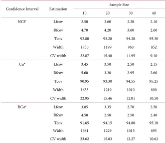
Table 1.Percentage (%) coverage failure of the true value Y, from the left (Lfcov) and from the right (Rfcov), % total coverage (Tcov), width of confidence intervals (Width) and widths coefficient of variation (CVwidth) as a function of the sample size (1 − a = 0.95).

Confidence Interval Estimation Sample Size

10 20 30 40

NCI* Lfcov 2.50 2.60 2.20 2.10

Rfcov 4.70 4.20 3.60 2.60

Tcov 92.80 93.20 94.20 95.30

Width 1730 1199 960 852

CV width 22.87 15.40 11.95 9.10

Cα* Lfcov 3.45 3.50 2.50 2.15

Rfcov 5.60 3.20 2.95 2.60

Tcov 90.95 93.30 94.55 95.25

Width 1653 1219 1010 890

CV width 22.95 15.46 12.01 10.50

BCα* Lfcov 3.85 3.35 2.70 2.50

Rfcov 4.50 2.50 2.50 2.40

Tcov 91.65 94.15 94.80 95.10

Width 1681 1229 1015 895

CV width 23.62 15.83 12.27 10.62

*by NCI (Normal), Cα (percentile method) and BCα (the bias-corrected and accelerated method).

The widths of confidence intervals as well as their variability decrease as the sample size increases for all estimated confidence intervals. Thus, the simulation iteration (5000) and sampling bootstrap (1500) numbers appear to be sufficient, ensuring consistency for all the estimates. With sample size 10, the overall cov-erage of the normal confidence interval is better (92.8%) than the covcov-erage of both bootstrap methods (90.95% and 91.65%), but the width (1730) of the nor-mal interval is greater from the widths of the bootstrap methods (1653 and 1681). At sample sizes, 20, 30 and 40 are not being observed significant differ-ences in the overall coverage of the three confidence intervals, with the BCα

method having slightly better coverage rates. The same is true for the confidence intervals widths, but now they are slightly smaller in the normal confidence in-terval. The variability of the confidence intervals is approximately the same (15.40, 15.46, 15.83). The 95% nominal coverage approach appears to be be-tween sample sizes 30 - 40 since in size 40 and the three confidence intervals it exceeds 95% nominal coverage. By comparing the two bootstrap methods, BCα

has a slightly better coverage up to sample size 30 and, correspondingly, slightly larger widths in confidence intervals.

(6)

(21.35%). Thus z-approach was preferred in order to keep at the same level the confidence interval widths up to less than 5%. A research result of Zhou & Dinh (2005) for the mean of the sample shows that if γˆ n<0.3, where γˆ is the skewness of the sample, the confidence interval which is based on t-approximation is good enough. The study found γˆ n<0.15 where γ =ˆ 0.46 and could be verified this result by considering BS as a simple random sampling n of N clus-ters of the population. The bootstrap confidence intervals were not well behaved for sample size 10, and this comes to an agreement with a relative result by

Schreuder & Williams (2000) for small sample sizes, although for different va-riables of the forest stand.

4. Conclusion

In conclusion, all three methods of constructing confidence intervals, to a large extent, almost approximate the nominal coverage in sample size 30, while pro-viding satisfactory coverage (>93%) in sample size 20. The normal confidence interval still has satisfactory coverage in the sample size 10, while for the same sample size, the bootstrap methods do not seem to perform well. The results came from a particular forest ecosystem with a clustered spatial distribution of trees and continuous management. However, it also needs research from other, different forest ecosystem structures in order to better evaluate the same confi-dence intervals, but also other types of conficonfi-dence intervals suggested by the li-terature.

Acknowledgements

This research has been financially supported by General Secretariat for Research and Technology (GSRT) and the Hellenic Foundation for Research and Innova-tion (HFRI) (Scholarship Code: 1319).

Conflicts of Interest

The authors declare no conflicts of interest regarding the publication of this pa-per.

References

Becker, R. A., Chambers, J. M., & Wilks, A. R. (1988). The New S Language: A Program-ming Environment for Data Analysis and Graphics. In Wadsworth and Brooks/Cole Advanced Books and Software. Berlin: Springer.

De Vries, P. G. (1986). Sampling Theory for Forest Inventory: A Teach-Yourself Course.

Berlin: Springer Science & Business Media. https://doi.org/10.1007/978-3-642-71581-5

Efron, B. (1982). The Jackknife, the Bootstrap, and Other Resampling Plans (Vol. 38). CBMS-NSF Regional Conference Series in Applied Mathematics, SIAM.

https://doi.org/10.1137/1.9781611970319

(7)

DOI: 10.4236/ojf.2020.101005 64 Open Journal of Forestry Eriksson, M. (1995). Design-Based Approaches to Horizontal-Point-Sampling. Forest

Science, 41, 890-907.

Gregoire, T. G., & Valentine, H. T. (2007). Sampling Strategies for Natural Resources and the Environment. London: Chapman and Hall/CRC.

https://doi.org/10.1201/9780203498880

Hájek, J. (1981). Sampling from a Finite Population (p. 247). New Yok:Marcel Dekker, Inc.

Horvitz, D. G., & Thompson, D. J. (1952). A Generalization of Sampling without Re-placement from a Finite Universe. Journal of the American Statistical Association, 47,

663-685. https://doi.org/10.1080/01621459.1952.10483446

James, G., Witten, D., Hastie, T., & Tibshirani, R. (2013). An Introduction to Statistical Learning with Applications in R. New York, Heidelberg, Dordrecht, London: Springer.

https://doi.org/10.1007/978-1-4614-7138-7_1

Kershaw Jr., J. A., Ducey, M. J., Beers, T. W., & Husch, B. (2016). Forest Mensuration

(5th ed.). New York: John Wiley & Sons. https://doi.org/10.1002/9781118902028 Lyons, M. B., Keith, D. A., Phinn, S. R., Mason, T. J., & Elith, J. (2018). A Comparison of

Resampling Methods for Remote Sensing Classification and Accuracy Assessment.

Remote Sensing of Environment, 208, 145-153. https://doi.org/10.1016/j.rse.2018.02.026

Magnussen, S. (2001). Saddlepoint Approximations for Statistical Inference of PPP Sam-ple Estimates. Scandinavian Journal of Forest Research, 16, 180-192.

https://doi.org/10.1080/028275801300088288

Matis, K. (2004). Forest Biometrics: II. Dendrometry (In Greek) (Vol. 2, 2nd ed.). Thes-saloniki, Greece: Pegasus.

McRoberts, R. E., Magnussen, S., Tomppo, E. O., & Chirici, G. (2011). Parametric, Boot-strap, and Jackknife Variance Estimators for the k-Nearest Neighbors Technique with Illustrations Using Forest Inventory and Satellite Image Data. Remote Sensing of En-vironment, 115, 3165-3174. https://doi.org/10.1016/j.rse.2011.07.002

Overton, W. S., & Stehman, S. V. (1995). The Horvitz-Thompson Theorem as a Unifying Perspective for Probability Sampling: With Examples from Natural Resource Sampling.

The American Statistician, 49, 261-268. https://doi.org/10.1080/00031305.1995.10476160

Palley, M. N., & Horwitz, L. G. (1961). Properties of Some Random and Systematic Point Sampling Estimators. Forest Science, 7, 52-65.

Robinson, A. P., & Hamann, J. D. (2010). Forest Analytics with R: An Introduction. Ber-lin: Springer Science & Business Media.

https://doi.org/10.1007/978-1-4419-7762-5_1

Roesch, F. A., Green, E. J., & Scott, C. T. (1993). An Alternative View of Forest Sampling.

Survey Methodology, Statistics Canada, 19, 199-204

Schreuder, H. T. (1970). Point Sampling Theory in the Framework of Equal-Probability Cluster Sampling. Forest Science, 16, 240-246.

Schreuder, H. T., & Williams, M. S. (2000). Reliability of Confidence Intervals Calculated by Bootstrap and Classical Methods Using the FIA 1-HA Plot Design.

https://doi.org/10.2737/RMRS-GTR-57

Schreuder, H. T., Gregoire, T. G., & Wood, G. B. (1993). Sampling Methods for Multire-source Forest Inventory. New York: John Wiley & Sons.

(8)

of Forest Research, 22, 1071-1078. https://doi.org/10.1139/x92-142

Stamatellos, G. (1991). Research of Forest Volume Estimation Possibilities with Two-Stages Sampling Designs (In Greek, with English Summary). Doctoral Thesis, Thessaloniki: Aristotle University of Thessaloniki.

Team, R. C. (2013). R: A Language and Environment for Statistical Computing.

Venables, W., & Ripley, B. D. (2000). S Programming. Berlin: Springer Science & Busi-ness Media. https://doi.org/10.1007/978-0-387-21856-4

Zhou, X. H., & Dinh, P. (2005). Nonparametric Confidence Intervals for the One- and Two-Sample Problems. Biostatistics, 6, 187-200.