The link between morphology and structure of brightest cluster galaxies:
automatic identification of cDs
Dongyao Zhao,
‹Alfonso Arag´on-Salamanca and Christopher J. Conselice
School of Physics and Astronomy, The University of Nottingham, University Park, Nottingham NG7 2RD, UK
Accepted 2015 January 24. Received 2015 January 20; in original form 2014 December 12
A B S T R A C T
We study a large sample of 625 low-redshift brightest cluster galaxies (BCGs) and link their morphologies to their structural properties. We derive visual morphologies and find that ∼57 per cent of the BCGs are cD galaxies,∼13 per cent are ellipticals, and∼21 per cent be-long to the intermediate classes mostly between E and cD. There is a continuous distribution in the properties of the BCG’s envelopes, ranging from undetected (E class) to clearly de-tected (cD class), with intermediate classes (E/cD and cD/E) showing the increasing degrees of the envelope presence. A minority (∼7 per cent) of BCGs have disc morphologies, with spirals and S0s in similar proportions, and the rest (∼2 per cent) are mergers. After carefully fitting the galaxies light distributions by using one-component (S´ersic) and two-component (S´ersic+Exponential) models, we find a clear link between the BCGs morphologies and their structures and conclude that a combination of the best-fitting parameters derived from the fits can be used to separate cD galaxies from non-cD BCGs. In particular, cDs and non-cDs show very different distributions in theRe–RFF plane, where Re is the effective radius and RFF (the residual flux fraction) measures the proportion of the galaxy flux present in the residual images after subtracting the models. In general, cDs have largerReand RFF values than ellip-ticals. Therefore we find, in a statistically robust way, a boundary separating cD and non-cD BCGs in this parameter space. BCGs with cD morphology can be selected with reasonably high completeness (∼75 per cent) and low contamination (∼20 per cent). This automatic and objective technique can be applied to any current or future BCG sample with good-quality images.
Key words: galaxies: clusters: general – galaxies: elliptical and lenticular, cD – galaxies: structure.
1 I N T R O D U C T I O N
The brightest cluster galaxies (BCGs) are the most luminous and massive galaxies in today’s Universe. Their stellar masses reach be-yond∼1011M
, and they reside at the bottom of the gravitational potential well of galaxy clusters and groups. Their formation and evolution relate closely to the evolution of the host clusters (Whiley et al.2008) and further tie to the history of large-scale structures in Universe (Conroy, Wechsler & Kravtsov2007). BCGs are typically classified as elliptical galaxies (Lauer & Postman1992), but a frac-tion of them possess an extended, low-surface-brightness envelope around the central region. These are referred to as cD galaxies (e.g. Dressler1984; Oegerle & Hill2001).
The surface-brightness profile of elliptical galaxies was orig-inally modelled using the empirical r1/4 de Vaucouleurs law
E-mail:[email protected]
(de Vaucouleurs1948). However, Lugger (1984) and Schombert (1986) showed that the r1/4 model cannot properly describe the
flux excess at large radii for most elliptical galaxies, and an addi-tional parameternwas introduced in the so-called S´ersic (r1/n) law
(S´ersic1963). For the most massive early-type galaxies, however, a single-S´ersic profile still does not reproduce their luminosity dis-tribution accurately. Gonzalez, Zabludoff & Zaritsky (2005) found that a sample of 30 BCGs were best fitted using a doubler1/4de
Vaucouleurs profile rather than a single-S´ersic law. Furthermore, Donzelli, Muriel & Madrid (2011) suggested that a two-component model with an inner S´ersic and an outer exponential profile is re-quired to properly decompose the light distribution of∼48 per cent of the BCGs in their 430 galaxy sample. A similar conclusion was obtained by Seigar, Graham & Jerjen (2007).
The light profiles of BCGs need to be explained by any success-ful model of galaxy formation and evolution. In hierarchical models of structure formation, a two-phase scenario is currently favoured. Hopkins et al. (2009) proposed that an early central starburst could
give rise to the bulge (elliptical) component of these galaxies, while the outer envelope was subsequently formed by the violent relax-ation of stars originating in galaxies which merged with the central galaxy. Alternatively, Oser et al. (2010) and Johansson, Naab & Ostriker (2012) suggested that intense dissipational processes such as cold accretion or gas-rich mergers could rapidly build up an ini-tially compact progenitor and, after the star formation is quenched, a second phase of slower, more protracted evolution is dominated by non-dissipational processes such as dry minor mergers to form the low-surface-brightness outskirts.
To shed light on the mechanism(s) leading to the formation of BCGs, especially of cD galaxies, we need to answer questions such as: Are elliptical and cD BCGs two clearly distinct and separated classes of galaxies? If so, are elliptical and cD BCGs formed by different processes or in different environments? Are the extended envelopes of cD galaxies intrinsically different structures which formed separately from the central bulge? To help answer these questions, in this paper we explore statistically how the visual clas-sification of BCGs into different morphological classes (e.g. ellipti-cal, cD; here referred to as ‘morphology’) relates to the quantitative structural properties of their light profiles (e.g. effective radiusRe,
S´ersic-indexn; generically called ‘structure’ in this paper). More-over, finding an automatic and objective way to select cD BCGs is non-trivial for future data bases and study. Recent study such as Liu et al. (2008) identified cD BCGs by Petrosian parameter profiles (Petrosian1976), but their method does not give an unambiguous criterion to separate cD galaxies from non-cD BCGs.
In this paper, we visually-classify 625 BCGs from the sample of von der Linden et al. (2007, hereafterL07) and fit accurate models to their light profiles. We find clear links between the visual mor-phologies and the structural parameters of BCGs, and these allow us to develop a quantitative and objective method to separate cDs galaxies from ellipticals BCGs. In a later paper (Zhao et al., in preparation), we will study how the visual morphology and struc-tural properties of BCGs correlate with their intrinsic properties (stellar masses) and their environment (cluster mass and galaxy density), and explore the implications that such correlations have for the formation mechanisms and histories of cDs/BCGs.
The paper is organized as follows. In Section 2, we introduce the BCG samples and the visual morphological classification of the BCGs. In Section 3, we describe the light distribution models and the fitting methods we use, and discuss how the results are affected by sky-subtraction uncertainties. This section also presents a quantitative evaluation of the quality of the fits. In Section 4, we present the structural properties of the BCGs in the sample. In Section 5, we introduce an objective diagnostic to separate cDs from non-cD BCGs using quantitative information from their light profiles. We summarize our main conclusions in Section 6.
2 DATA
2.1 BCG catalogue and images
To study the structural properties of BCGs in galaxy groups and clusters, we use the BCG catalogue published byL07. The groups and clusters that host these BCGs come from the C4 cluster cat-alogue (Miller et al.2005) extracted from the Sloan Digital Sky Survey (SDSS; York et al.2000) third data release spectroscopic sample. The cluster-finding algorithm used to build the C4 catalogue identifies clusters as overdensities in a seven-dimensional param-eter space of position, redshift, and colour, minimizing projection effects. The C4 catalogue gives a very clean widely-used cluster
sample which is well supported by simulations. Based on the C4 catalogue,L07restricted their cluster sample to the 0.02≤z≤0.10 redshift range to avoid problems related to the 55 arcsec ‘fibre collision’ region of SDSS. Within each cluster, L07 applied an improved algorithm to identify the BCG as the galaxy being clos-est to the deepclos-est point of the potential well of the cluster (see L07for a detailed discussion of this identification), and developed an iterative algorithm to measure the cluster velocity dispersion σr200within the virial radiusR200.1The catalogue created byL07
contains 625 BCGs in galaxy groups and clusters with redshifts 0.02≤ z≤0.10 spanning a wide range of cluster velocity dis-persions, from galaxy groups (σr200≤200 km s−1) to very massive
clusters (σr200∼1000 km s−1). 75 per cent of the BCGs inL07are in
dark matter haloes withσr200≥309 km s−1, where the completeness
of the haloes identified by the C4 algorithm is expected to be above 50 per cent. Obviously, for larger halo masses the completeness is higher.
The images we use to classify the BCGs and analyse their struc-tural properties come from the SDSS Seventh Data Release (DR7)
r-band images. We also use SDSS-DR7g-band images of the BCGs in Section 4.1. The BCG catalogue used in this paper together with their main properties is presented in Appendix A.
2.2 Visual classification
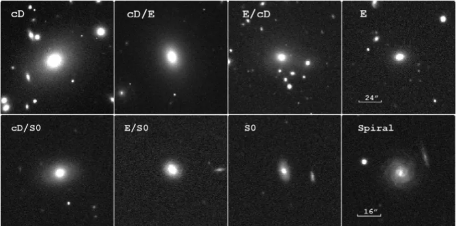
The 625 BCGs in L07sample were visually classified by care-ful inspection of the SDSS images. BCGs were displayed using a logarithmic scale between the sky level and the peak of the surface-brightness distribution. The contrast was adjusted manually to ensure that the low-surface-brightness envelopes were revealed if present. cD galaxies are identified by a visually extended envelope, while the envelope is not visible in our elliptical BCGs. Finally, the BCGs were classified into three main types: 414 cDs, including pure cD (356), cD/E (53), and cD/S0 (5); 155 ellipticals, including pure E (80), E/cD (72), and E/S0 (3); 46 disc galaxies, containing spirals (24) and S0s (22). The main morphological classes of BCGs are illustrated in Fig.1. There are also 10 BCGs undergoing major mergers, but we will not discuss them in this paper in any detail.
Over half of the BCGs in the sample are classified as cDs. Sepa-rating cD BCGs and non-cD elliptical BCGs is a very hard problem since there is no sharp distinction between these two classes (e.g. Patel et al.2006; Liu et al.2008). Detecting the extended stellar envelope that characterises cD galaxies depends not only on its dominance, but also on the quality and depth of the images, and on the details of the method(s) employed. We used intermediate classes such as cD/E (probably a cD, but could be E) and E/cD (probably E, but could be cD) to account for the uncertainty inherent in the visual classification.
Our careful inspection of the images clearly reveals that there is a wide range in the brightness and extent of the envelopes. There seems to be a continuous distribution in the envelope properties, ranging from undetected (pure E class) to clearly detected (pure cD class), with the intermediate classes (E/cD and cD/E) showing in-creasing degrees of envelope presence. This continuous distribution in envelope detectability will also be made evident in the structural analysis carried out later in this paper. The classification we present here does not intend to be a definitive one since such a thing is probably unachievable. Our aim is to obtain a homogeneous and
1R
200is the radius within which the average mass density is 200ρc, where
Figure 1. Examples of the main morphological classes of BCGs in our sample (cD, cD/E, E/cD, E, cD/S0, E/S0, S0, Spiral) illustrating the gradual transition between classes. The images are displayed using a logarithmic surface-brightness scale.
systematic visual classification of the BCGs and then study how such classification correlates with quantitative and objective struc-tural properties of the BCGs. The visual morphological types of all the galaxies in the sample are presented in Appendix A.
We checked the effect that the redshift of BCGs may have on the visual classification. cDs might be mistakenly identified as elliptical if they are more distant since the extended low-surface-brightness envelope may be harder to resolve at higher redshifts. Fig.2 illus-trates the redshift distribution of the three main types. cD galaxies generally share the same redshift distribution with elliptical BCGs, especially atz≥0.05. Atz <0.05, we identify a slightly higher proportion (by∼10 per cent) of cD galaxies. However, if we com-pare the structural properties of cD and elliptical BCGs which are at z≥0.05, the results we obtain do not significantly differ from those using the full-redshift sample. As an additional check, we artificially redshifted some of the lowest redshift galaxies (z∼0.02–0.03) to z=0.1, the highest redshift of the sample, taking into account cos-mological effects such as surface-brightness dimming. Because the redshift range of the BCGs we study is very narrow, the effect on the images is minimal and does not have any significant impact on the visual classification. We are therefore confident that our visual clas-sification is robust and that in the relatively narrow redshift range explored here any putative redshift-related biases will not affect our results.
3 Q UA N T I TAT I V E C H A R AC T E R I Z AT I O N O F A B C G S T R U C T U R E
The surface-brightness profiles of galaxies provide valuable infor-mation on their structure and clues to their forinfor-mation. It has become customary to fit the radial surface-brightness distribution using theo-retical functions which have parameters that include a measurement of size (e.g. half-light radius or scalelength), a characteristic surface brightness, and other parameter(s) describing the shape and proper-ties of the surface-brightness profiles. In this paper, we useGALFIT
(Peng et al.2002) to fit the 2D luminosity profile of each BCG using two parametric models, and thus determine the best-fitting
parame-Figure 2. Redshift distribution for BCGs with different morphological types. The red solid line corresponds to cD BCGs, the green dashed line to ellipticals, and the blue dotted line to disc (spiral and S0) BCGs. A Kolmogorov–Smirnov test indicates that the redshift distributions of cD and elliptical BCGs are only different at the∼2.4σlevel. cD galaxies share the same redshift distribution with elliptical BCGs atz≥0.05, while there are proportionally∼10 per cent more cD galaxies atz <0.05.
[image:3.595.311.538.327.582.2]We explore two models to represent the luminosity profile of the BCGs. A model commonly used to fit a variety of galaxy light profiles is the generalization of ther1/4de Vaucouleurs (1948) law
introduced by S´ersic (1963). The S´ersic model has the form
I(r)=Ieexp{−b[(r/Re)1/n−1]}, (1)
whereI(r) is the intensity at distancerfrom the centre,Re, the
ef-fective radius, is the radius that encloses half of the total luminosity,
Ieis the intensity atRe,nis the S´ersic index representing
concentra-tion, andb2n−0.33 (Caon, Capaccioli & D’Onofrio1993). The S´ersic function provides a good model for galaxy bulges and mas-sive elliptical galaxies. Since BCGs are mostly early-type galaxies, it is reasonable to fit their structure with single-S´ersic models first. Subsequently, in order to explore the complexity introduced by the extended envelopes of cD galaxies, we will also fit the light profile of BCGs adding an additional exponential component to the S´ersic profile. Adding this exponential component is the simplest way to describe the ‘extra-light’ from the extended envelope. Note that the exponential profileI(r)=I0exp (−r/rs) is just a S´ersic model with n=1. The models assume that the isophotes have elliptical shapes, and the ellipticity and orientation of each model component are parameters determined in the fitting process.
In order to runGALFIT, we require a postage stamp image for each
BCG with appropriate size to measure its structure over the full extent of the object, a mask image with the same size as the stamp image, an initial guess for the fitting parameters, an estimate of the background sky level, and a point spread function (PSF). Details on how these ingredients are produced and the fitting procedures are given below.
3.1 Pipeline for one-component fits:GALAPAGOS
We runGALFITusing theGALAPAGOSpipeline (Barden et al.2012). GALAPAGOShas been successfully applied to a wide variety of
ground-and space-based images (H¨aussler et al.2007; van der Wel et al. 2012,2014; Huertas-Company2013; Lani et al.2013). We applied the version ofGALAPAGOS1.0 to fit the SDSSr-band images of the
BCGs in our sample. The starting point are SDSS images with a size of 2047×1488 pixels. For each BCG, the pipeline carries out four main tasks before runningGALFITitself: (i) detection of all
the sources present in the image; (ii) cutting out the appropriate postage stamp and preparing the mask image; (iii) estimation of the sky background; (iv) preparation of the input file forGALFIT.
After completing these tasks,GALAPAGOSwill runGALFITusing the
appropriate images and input parameters. We describe now these tasks in detail.
(i) Source detection:SEXTRACTOR (Bertin & Arnouts1996) is
used to detect galaxies in the SDSS images. A set of configura-tion parameters defines how SEXTRACTORdetects sources. The
val-ues of the SEXTRACTORinput parameters follow Guo et al. (2009):
DETECT_MINAREA=25, DETECT_THRESH=3.0, and DE-BLEND_MINCONT=0.003. This set of parameters were tested to perform well on SDSSr-band images so that the bright and ex-tended BCGs were isolated from other sources without artificially deblending them into multiple components. SEXTRACTORalso
pro-vides estimates of several properties for the target BCGs and nearby objects such as their magnitude, size, axis ratio, and position angle. These values are used to calculate the initial guesses of the model parameters that are needed as inputs byGALFIT.
(ii) Postage stamp creation:GALAPAGOS cuts out a rectangular
postage stamp centred on the target BCG which will be used by
GALFITas input image. We define the ‘Kron ellipse’ for a galaxy
im-age as an ellipse whose semimajor axis is the Kron radius2(R kron),
with the ellipticity and orientation determined by SEXTRACTOR. The
postage stamp size is determined in such a way that it will fully contain an ellipse 3.5 times larger than the Kron ellipse, i.e. its semimajor axis is 3.5Rkron, and has the same ellipticity and
orienta-tion. The 3.5 factor represents a compromise between computational speed and ensuring that virtually all the BCG’s light is included in the postage stamp. At this stage, a mask image is also created, identifying and masking out all pixels belonging to objects in the postage stamp which will not be simultaneously fitted byGALFIT.
The aim is to reduce the computational time by excluding objects too far from the BCG or too faint to have any significant effect on the fit. Following Barden et al. (2012), an ‘exclusion ellipse’ is de-fined for each galaxy with a semimajor axis 1.5Rkron+20pixels, and
the same ellipticity and orientation as the Kron ellipse.GALAPAGOS
masks out all objects whose exclusion ellipse does not overlap with the exclusion ellipse of the target BCG. These objects are deemed to be too far away from the BCG to require simultaneous fitting. Furthermore, all objects more than 2.5 mag fainter than the BCG are also masked out since they are too faint to affect the BCG fit. The pixels that belong to these objects according to the SEXTRACTOR
segmentation maps are masked out and excluded from the fits. All the remaining objects will be simultaneously fitted byGALFITat the same time as the BCG. For a detailed description of this process and a justification of the parameter choice, see Barden et al. (2012).
(iii) Sky estimation:accurate estimates of the sky background level is crucial when fitting galaxy profiles, particularly when inter-ested in the low-surface-brightness outer regions. Overestimating the sky level will result in the underestimation of the galaxy flux, size, and S´ersic indexn, and vice versa.GALAPAGOSuses a flux growth curve method to robustly estimate the local sky background around the target galaxy. SDSS DR7 also provides a global sky value for the whole 2047×1488 image frame and local sky values for each galaxy. The SDSS PHOTO pipeline estimates the sky background using the median flux of all the pixels in the image after 2.33σ -clipping. However, according to the SDSS-III website, the version of PHOTO used in DR7 and earlier data releases tended to overes-timate both the global and local sky values. The sky measurement is improved by SDSS-III in later data releases, but since we use the images from DR7 we cannot use the SDSS sky value with enough confidence. H¨aussler et al. (2007) demonstrated that the sky mea-surement thatGALAPAGOSproduces is highly reliable for single-band
fits because it takes into account the effect of all the objects in the image. Therefore, in this study we use the local sky background estimated byGALAPAGOS. The accurate sky measurement provided
byGALAPAGOSindicates that we can reach a surface-brightness limit in therband of∼27 mag arcsec−2. This is deep enough to study
the faint extended structures of BCGs. For each galaxy, its local sky background is included in theGALFITinput file and is fixed during
the fitting procedure. Given the importance of accurate sky subtrac-tion, in Section 3.2 we will carry out an explicit comparison of our results using SDSS andGALAPAGOSsky estimates.
(iv)GALFIT Input: GALAPAGOSproduces an input file which
in-cludes initial guesses for the fitting parameters based on the SEXTRACTOR output. As mentioned above, all objects which are not masked out are fitted simultaneously using a S´ersic model. The
2In this paper, we use the following definition of ‘Kron radius’:
Rkron=2.5r1, wherer1is the first moment of the light distribution (Kron
initial-guess model parameters for these nearby companions are also determined from SEXTRACTOR. In order to obtain reasonable results,
we impose some constraints on the acceptable model parameter range. Our constrains on position, magnitude, axis ratio, and posi-tion angle follow H¨aussler et al. (2007). Additionally, the half-light radiusReis constrained within 0.3≤Re≤800 pixels. This prevents
the code from yielding unreasonably small or large sizes. Since the pixel size of the SDSS images is 0.396 arcsec,Reis constrained to
be larger than 0.12 arcsec, which is much smaller than the PSF, and smaller than half the size of the original input images, reasonable for the range of redshifts explored. In the originalGALAPAGOSpipeline,
the constraint on the S´ersic index is 0.2≤n≤8. These are reason-ably conservative limits, since normal galaxies withn>8 are rarely seen and are often associated with poor model fits. However, some studies have shown that very luminous elliptical galaxies withn>8 do exist (e.g. Graham et al.2005), therefore for the target BCGs we allownto be as large as 14 to keep the fits as free as possible. For the companion galaxies, which are fitted simultaneously, we still keep the constraint 0.2≤n≤8. The final ingredient needed byGALFITis
a PSF image appropriate for each BCG. These are extracted from the SDSS DR7 data products3according to the photometric band
used and the position of the BCG on the SDSS image.
3.2 Effect of the sky background subtraction: comparing SDSS andGALAPAGOSsky estimates
As described in Section 3.1, in this study we rely on the sky mea-surements provided byGALAPAGOS. However, it is important to test
the effect that the choice of sky background has on our results. We do this by comparing the fitted S´ersic model parametersnandRe
using theGALAPAGOSand SDSS sky estimates. As mentioned before,
SDSS DR7 provides a global sky value for the whole 2047×1488 image and local sky values for each galaxy. Guo et al. (2009) found that the local background estimates are generally larger than the global ones due to contamination from the outskirts of extended and bright sources, making them unreliable. We therefore restrict our comparison to the global SDSS sky values. We fit the BCG light profiles twice using exactly the same procedure and input pa-rameters (see Section 3.1) but changing only the sky background estimates. The first set of fits use the GALAPAGOS-determined sky
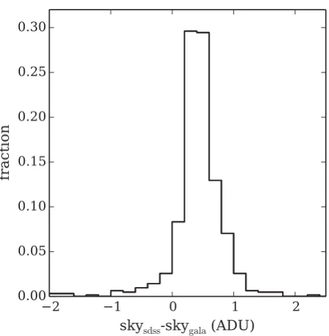
values, while the second set use the SDSS DR7 global ones. Fig.3shows the distribution of the difference between the SDSS DR7 global sky and the sky measured byGALAPAGOS. It is clear that the SDSS global sky is generally larger than the local sky from
GALAPAGOS. The effect from different sky values on the best-fitting structural parameters (S´ersic indexn and effective radiusRe) is
shown in Fig.4. It is clear that the SDSS larger sky values result in the values ofnsdssandre,sdssbeing smaller than the corresponding GALAPAGOSones. The effect becomes more severe for those BCGs
with large nandRe, most of which are cD galaxies. This means
the overestimated sky values would particularly affect the mea-surements on the low-surface-brightness envelopes of cD galaxies. Although it is difficult to know a priori which thetruevalue of the sky background is, based on the fact that the SDSS-III provides ev-idence that DR7 sky values are overestimated while H¨aussler et al. (2007) showed reasonable proof of the reliability of theGALAPAGOS
sky measurements, in what follows we will therefore trust and use theGALAPAGOS-determined sky values.
[image:5.595.308.547.52.296.2]3http://www.sdss.org/DR7/products/images/read_psf.html
Figure 3. Distribution of the difference between the SDSS DR7 global sky and theGALAPAGOS-measured sky values. In general, SDSS overestimates the
sky background. The average sky value measured byGALAPAGOSin the SDSS
[image:5.595.306.545.381.634.2]r-band BCG images is 140.8 ADU, corresponding to a surface brightness of∼20.9 mag arcsec−2.
Figure 4. Comparison on the best fitnandRefrom single-S´ersic models
using the SDSS andGALAPAGOS-measured sky estimates. Solid and open red circles correspond to pure cD and other cD galaxies (cD/E and cD/S0) respectively; solid and open green diamonds correspond to pure and other (E/cD and E/S0) elliptical BCGs respectively; solid blue triangles represent S0s and open ones are spirals. It shows that the SDSS overestimation of the global sky result in the values ofnsdssandre,sdssbeing smaller than the
3.3 Two-component fits
Although the light profiles of many early-type galaxies can be re-produces reasonably well with single-S´ersic models, the extended envelopes of cD galaxies may require an additional component. We therefore fitted all the BCGs byGALFITusing a two-component
model consisting of a S´ersic profile plus an exponential. The input postage stamp, mask image, PSF, and sky values required byGALFIT
remain the same as for the single-S´ersic fits. To ensure that we are fitting exactly the same light distribution, the location of the centre of the BCG is fixed to theX- andY-coordinates determined in the single fit, and we also force the initial guesses of the model param-eters to be the single-component fit results. The BCG companions are simultaneously fitted still with single-S´ersic profiles but with initial-guess parameters determined by the single-profile fits.
3.4 Residual flux fraction and reducedχ2
Although the models we are fitting are generally reasonably good descriptions of the BCG light profiles, real galaxies can be more complicated, with additional features and structures such as star-forming regions, spiral arms, and extended haloes. It is therefore desirable to quantify how good the fits are and what residuals re-main after subtracting the best-fitting models. A visual inspection of the residual images can generally give a good feel for how good a fit is, and sometimes tell us whether an additional component or components are required. However, more quantitative, repeatable, and objective diagnostics are also needed. The residual flux frac-tion (RFF; Hoyos et al.2011) provides one such diagnostic. It is defined as
RFF=
i,j∈A|Ii,j−Ii,jmodel| −0.8×i,j∈Aσi,jbkg
i,j∈AIi,j , (2)
whereAis the particular aperture used to calculate RFF. WithinA,
Ii,jis the original flux of pixel (i.j),Ii,jmodelis the model flux created
byGALFIT, andσi,jbkgis the rms of the background. RFF measures the
fraction of the signal contained in the residual image that cannot be explained by background noise. The 0.8 factor ensures that the expectation value of the RFF for a purely Gaussian noise error im-age of constant variance is 0.0. See Hoyos et al. (2011) for details. Obviously, this diagnostic can be applied to both single-S´ersic and two-component profiles, or any other model. The apertureAwe use to calculate RFF is the ‘Kron ellipse’ defined in Section 3.1 (an ellipse with semimajor axisRkronand the ellipticity and orientation
determined by SEXTRACTORfor the BCG).i,j∈AIi,j, the
denomina-tor of equation (2), is computed as the total BCG flux contained inside the Kron ellipse, which is one of the SEXTRACTORoutputs,
and therefore independent of the model fit.
Since BCGs usually reside in dense environments, sometimes there are some faint nearby objects contained within the Kron el-lipse that have not been fitted byGALFIT(those more than 2.5 mag
fainter than the BCG, see Section 3.1). These objects will be present in the residual image. Moreover, brighter companions that have been simultaneously fitted may also leave some residuals due to inaccu-racies in their fits. Therefore, even if the BCG light distribution has been accurately fitted, RFF can be affected by the residuals from the companion galaxies, failing to provide an accurate measure of the quality of the fit. To minimize the effect from companion galax-ies on RFF, we mask out the pixels belonging to all companions within the Kron ellipse using SEXTRACTORsegmentation maps. The
RFF will therefore measure the residuals from the BCG fit alone, excluding, as far as possible, those belonging to nearby galaxies.
An additional measurement of the fit accuracy is the reducedχ2,
which is minimized byGALFITwhen finding the best-fitting models. It is defined as
χ2
ν =
1 Ndof
i,j∈A
(Ii.j−Ii,jmodel)2
σ2
i,j ,
(3)
whereAis the aperture used to calculateχ2
ν, Ndofis the number
of degrees of freedom in the fit,Ii,jis the original image flux of
pixel (i,j).Imodel
i,j represents, for each pixel, the sum of the flux of
the models fitted to all the galaxies in the aperture, andσi,jis the
noise corresponding to pixel (i,j). This noise is calculated byGALFIT
taking into account the contribution of the Poisson errors and the read-out noise of the image (Peng et al.2002).
Similarly to RFF,χ2
ν also measures the deviation of the fitted
model from the original light distribution. The value of χ2
ν that
GALFITminimises to find the best-fitting model is calculated over
the whole postage stamp, and includes contributions from all the objects fitted. To make sure that we only take into account the contribution toχ2
νfrom the BCG fit, we calculate it within the Kron
ellipse of the BCG, masking out the nearby objects as we did when calculating RFF.
The choice of aperture (Kron ellipse with semimajor axis ofRkron)
over which we evaluate RFF andχ2
ν represents a good compromise
between covering a large fraction of the galaxy light while mini-mizing the impact of close companions. We carried out several tests to evaluate the sensitivity of our results to the changes in aperture size. If we reduce the semimajor axis of the aperture by 20 per cent or more we lose significant information on the extended halo of BCGs, which we must avoid. If we increase the semimajor axis of the aperture by 20 per cent or more, we potentially increase the sensitivity to the galaxy haloes but in the crowded central cluster regions contamination from companion galaxies becomes a serious problem, generally increasing RFF andχ2
ν. Changes in the aperture
semimajor axis within±20 per cent would have no effect on the conclusions of this paper.
3.5 Evaluating one-component and two-component fits
Since RFF andχ2
νcan quantify the residual images after subtracting
the model fits, we attempt to use them to assess whether a one-component (S´ersic) fit or a two-one-component (S´ersic+Exponential) fit is more appropriate to describe the light profile of individual BCGs. In order to do this, we first evaluate the effectiveness of RFF and χ2
ν at quantifying the goodness-of-fit. We visually examine the fits
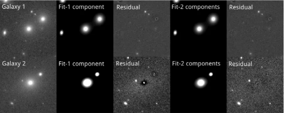
and residuals obtained from both one- and two-component models for all the BCGs in our sample. In some cases, two of which are illustrated in Fig.5, it is obvious which model is clearly favoured.
Figure 5. Example of one-component (S´ersic) fits and two-component (S´ersic+Exponential) fits for 1C and 2C BCGs, respectively. From left to right, the panels show the original image, the one-component model, the residuals after subtracting the one-component fit, the two-component model, and the residuals after subtracting the two-component fit. The upper panels show a 1C BCG where a one-component fit does a good job and adding a second component does not visibly improve the residuals. The lower panels show a 2C BCG, where the one-component residual exhibits clear excess light at large radii, suggesting that a second component is necessary. Indeed, the two-component residual is much better for this BCG.
and 25 2C BCGs. Since we want to test the sensitivity of RFF and χ2
ν, we concentrate for now on this small but robust subsample. The
rest of the BCGs (537) cannot be confidently classified into 1C or 2C BCGs because it is too hard to tell visually due to the residuals containing significant structures which cannot be accurately fitted by such simple models.
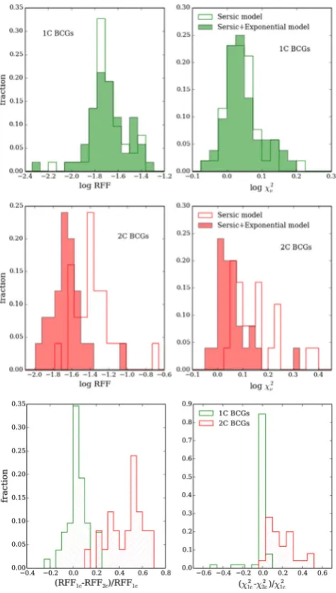
Fig.6presents a comparison of the RFF andχ2
νvalues for the
one-and two-component fits of the 53 1C BCGs one-and 25 2C BCGs. For 1C BCGs, the RFF andχ2
ν distributions of one- and two-component
fits are virtually indistinguishable. Neither RFF nor χ2
ν improve
significantly when the second component is added. However, RFF andχ2
ν are significantly smaller for the two-component fits of 2C
BCGs. It is clear therefore that the quantitative information that RFF andχ2
νprovide agrees very well with the visual assessments of
the fits. Both RFF andχ2
ν are sensitive to changes in the residuals,
but RFF appears to be more sensitive. As shown in the bottom panels of Fig.6, the improvement in the two-component fit for 2C BCGs is around 40–60 per cent when measured by RFF, while it is only∼20 per cent when measured byχ2
ν. A further useful piece
of information obtained from this test is that the typical values of log RFF and logχ2
ν for fits deemed to be good by visual inspection
are log RFF −1.7+−00..1106, and of logχν20.042+−00..033025(median+/−
first and third quartiles of the parameter distributions).
As mentioned before, the majority of the BCGs cannot be visually classified into 1C or 2C BCGs with high certainty because their light distributions are too complex to be accurately represented by such simple models. Nevertheless, we can use the quantitative information provided by RFF andχ2
ν to gauge to what extent the
BCGs are better fit by a two-component model than by a one-component model. This will be discussed later.
We would like to point out that this is the first time that the resid-ual flux is calculated consideringonlythe contribution of the target galaxies when estimating both RFF andχ2
ν, explicitly excluding the
contribution due to the companion galaxies. For instance, Hoyos et al. (2011) also used RFF to evaluate the goodness-of-fit, but they measured the residuals over all pixels within a specific area around the target galaxies, without excluding nearby companions. Simi-larly, theχ2
ν values fromGALFIThave also been applied to evaluate
which fitting model is better (e.g. Bruce et al.2012), but the effect
of nearby objects on theχ2
ν values was also overlooked. Using the
2C BCG sample, we assessed the importance of this improvement. If the RFF andχ2
ν are calculated considering the residuals in all the
pixels inside the relevant aperture, the RFF andχ2
ν distributions for
the two-component fits of 2C BCGs cannot be distinguished from the one-component results. The effect of the contribution to the residuals from companion galaxies is so severe that it renders such a comparison useless. Our method therefore represents a significant step forward. It is extremely important to exclude the contribution of the companion galaxies when calculating RFF andχ2
νin this kind
of analysis.
4 S T R U C T U R A L P R O P E RT I E S O F B C G s
Our morphologically-classified BCGs provide a large sample to statistically study their structural properties and link them to their morphological properties. In what follows we consider the three main morphological classes of BCGs: cDs (including all BCGs classified as pure cD, cD/E, and cD/S0); ellipticals (including pure E, E/cD, and E/S0), and disc (spiral and S0) BCGs. The 10 BCGs classified as mergers are excluded (see Section 2.2 for details). We decided to include the galaxies with ‘uncertain’ morphologies (such as cD/E and E/cD) in our analysis to reflect the difficulties involved in visual classification. However, to ensure the robustness of our analysis, at every stage we have checked that considering only ‘pure’ cD and elliptical BCGs (i.e. excluding the cD/E, cD/S0, E/cD, and E/S0 classes) would not change our conclusions.
Since most BCGs are early-type galaxies, we will first consider and discuss single-S´ersic models when fitting their SDSSr-band images. We will subsequently use S´ersic+Exponential models to see whether the fits are improved. But before embarking in the analysis of the parameters derived from these model fits, we first evaluate their uncertainties.
4.1 Structural parameter uncertainties
The parameter uncertainties thatGALFITreports are calculated using
Figure 6. The top four panels show the distribution of log RFF (left) and logχ2
ν (right) for single-S´ersic (open histograms) and S´ersic+Exponential (solid histogram) fits. The two uppermost panels correspond to the 53 1C BCGs, while the middle panels correspond to the 25 2C BCGs. The two bottom panels show the difference in RFF andχ2
ν between one-component and two-component models for both sets of BCGs. Clearly, the RFF and
χ2
νdistributions of one- and two-component fits are virtually indistinguish-able for 1C BCGs. However, RFF andχ2
ν tend to be significantly smaller for the two-component fits of 2C BCGs. Typical values for good fits are log RFF −1.7+−00..1106, and logχ2
ν0.042−+00..033025(median+/−the first and
third quartiles of the parameters). Both RFF andχν2are sensitive to the magnitude of the residuals, but RFF is appears to be significantly more sensitive.
et al.2010). These formal uncertainties are only meaningful when the model provides a good fit to the image, in which case the fluctu-ations in the residual image are only due to Poisson noise. However, for real galaxy images the residual images contain not only Poisso-nian noise, but also systematics from non-stochastic and stochastic factors due to additional components not included in the fitting func-tion (e.g. spiral arms, star-forming regions), asymmetries, shape mismatch, flat-fielding errors and so on. These non-random factors usually dominate the uncertainty of the parameters, and the uncer-tainties inferred from the covariance matrices are only lower-limit
estimates (Peng et al.2010). Therefore, if we rely on the errors reported byGALFITthe uncertainties in the structural parameters of
the BCGs could be severely underestimated. Indeed, these formal errors seem unrealistically small: typicalGALFITuncertainties forRe
andnare only∼1–2 per cent. A more robust and realistic way of determining these uncertainties is clearly needed.
We have measured the structural parameters of the BCGs in our sample using the SDSSr-band images. Independent measurements can also be obtained using the SDSSg-band images. In principle, the structural parameters could be wavelength dependent. However, theg−rcolours of massive early-type galaxies with old stellar pop-ulations are quite spatially uniform and do not change much from galaxy-to-galaxy (e.g. Fukugita, Shimasaku & Ichikawa1995). Fur-thermore, morphologicalk-corrections are negligible for early-type galaxies between these two bands (e.g. Taylor-Mager et al.2007), so it is reasonable to expect that the intrinsic structural parameters will not change much betweengandrbands. Therefore, any differ-ences in the measured parameters between these two bands should be largely dominated by measurement errors. Moreover, if there are significant wavelength-dependent differences in the measured pa-rameters that are driven by real physical differences, it is reasonable to expect that these may correlate with other galaxy properties such as their colour, morphology, redshift, cluster velocity dispersion, etc. No such correlations were found, so we are confident that the intrinsic differences are not significant in these two bands.
We useGALAPAGOSto fit the SDSSg-band images of the BCGs
in our sample in exactly the same way as we did for ther-band images. Fig. 7shows a comparison of the Re and RFF1c values
obtained in both bands. Similar comparisons were carried out for the rest of the structural parameters. The scatter around the 1-to-1 relations is due, in principle, to both intrinsic wavelength-dependent differences and measurement errors. Since, as we have argued, the intrinsic differences are not expected to be significant between these two bands, the measurement errors should dominate the scatter. We can thus use this scatter as an estimate of realistic, albeit perhaps marginally pessimistic, parameter uncertainties. The average errors areδ(n)0.9,δ(logRe)0.16, andδ(log RFF1c)0.13.
The right-hand panel of Fig.7shows that the errors inReand RFF
are not correlated. This is an important point since these two are the main parameters that we will use as diagnostics in our analysis in Section 5.
4.2 Single-S´ersic models
We analyse now the behaviour of four parameters derived from the best-fittng single-S´ersic models along with the morphological clas-sifications. Two of them, the S´ersic indexnand the effective radius
Re, provide information on the intrinsic properties of the BCGs.
The other two, RFF andχ2
ν, show how well the models fit the real
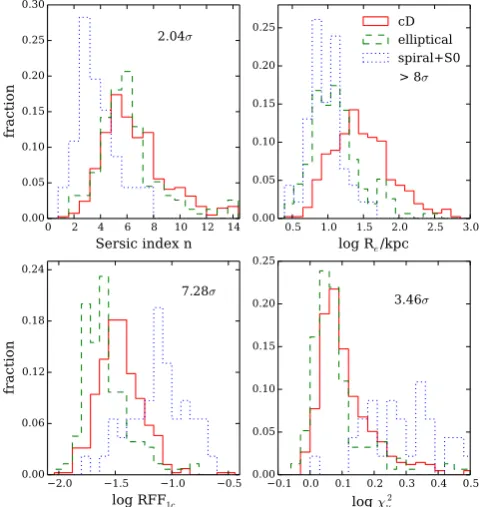
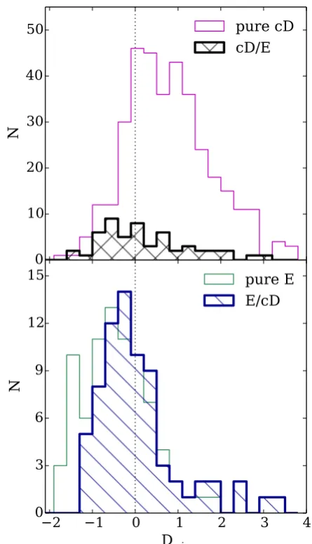
light distribution of the BCGs and also provide information about their detailed structure. The values of these parameters are listed in Appendix A. Fig.8shows the distribution of these parameters for the three main BCG morphologies. Theσ value in each panel indi-cates the significance (confidence level) of the observed differences between the cD and elliptical BCG parameter distributions. These are derived from two-sample Kolmogorov–Smirnov (K–S) tests.
4.2.1 S´ersic index n
Figure 7. Comparison of theRe(left-hand panel) and RFF1c(middle panel) values obtained in both the SDSSg- andrbands. The solid lines correspond to
the 1-to-1 relations. The right-hand panel shows log (Re,g/Re,r) versus log (RFF1c,g/RFF1c,r). The error bars in the bottom-right corner are derived from the
rms scatter of each parameter.
Figure 8. Distribution of the S´ersic indexn(upper left), effective radiusRe
(upper right), log RFF1c(lower left), and logχν2(lower right) from
single-S´ersic fits for the BCGs divided by morphology. The red solid line cor-responds to cD galaxies, the green dashed line to ellipticals, and the blue dotted line to spirals and S0s. Theσ value in each panel indicates the sig-nificance (confidence level) of the observed differences between the cD and elliptical BCG parameter distributions. These are derived from two-sample Kolmogorov–Smirnov tests.
panel of Fig.8presents thendistributions for the three main BCG morphologies. It is clear that disc (spiral and S0) BCGs tend to have smaller values ofn, as expected. However, thendistribution for disc BCGs is skewed towards larger values (n3) than those of the nor-mal disc galaxy population (e.g.n=2.5 in Shen et al.2003). This is because most disc BCGs are early-type bulge-dominated spirals and S0s. Elliptical and cD BCGs tend to have largernvalues (n≥4). The ndistributions of cD and elliptical BCGs are quite similar. A K–S test indicates that the distributions are not significantly dif-ferent: the significance of any possible difference is just 2.04σ.
4.2.2 Effective radius Re
The effective radius Re is a measurement of the extent (or size)
of the light distribution. The upper-right panel of Fig.8shows the distributions of logRe. Disc BCGs tend to have relatively small
sizes, and the vast majority of them (∼85 per cent) haveResmaller
than∼15h−1 kpc. About 75 per cent of the elliptical BCGs also
haveRe15h−1kpc, while cD galaxies tend to be significantly
larger. More than 60 per cent of cDs haveRe15h−1kpc. A K–S
test demonstrates that the difference inRedistributions between cD
and elliptical BCGs is very significant. This suggests thatRecould
be a good discriminator to separate cD and elliptical BCGs.
4.2.3 Residual flux fraction and reducedχ2
The lower-left panel of Fig.8presents the RFF1cdistributions in
a log10scale, where RFF1cdenotes RFF for one-component
mod-els. The RFF1cof disc BCGs has a much broader distribution and
reaches significantly larger values than those of cDs and ellipticals. This reflects the fact that a single-S´ersic model is not a good repre-sentation of the light distribution of galaxies with clear discs, spiral arms, and star-forming regions. Early-type BCGs have smoother light distributions that can be reasonably well reproduced with a S´ersic profile, and their RFF1ctend to be smaller. However, there
are statistically significant differences between the RFF1c
distri-butions of cD and elliptical BCGs. About 60 per cent of elliptical BCGs have RFF1cvalues in the range corresponding to good fits
(see Section 3.5 and Fig.6), while just∼25 per cent of cD galaxies do. This suggests that most elliptical BCGs can be well represented by single-S´ersic models, while most cD galaxies are harder to model with such a simple profile. Since an extended envelope is a general property of cD galaxies, their deviation from a single-S´ersic pro-file may be due, at least partially, to this extended envelope. This suggests that an additional model component may be required for them. We will re-visit two-component models in Section 4.3. The clear difference in RFF suggests that RFF could be another good discriminator to separate cD and elliptical BCGs.
Similar conclusions can be reached from the distributions ofχ2
ν
shown in the lower-right panel of Fig.8, albeit less clearly. This is not surprising since, as shown in Section 3.5, both RFF and χ2
ν measure the strength of the residuals, butχν2 is significantly
less sensitive. Therefore, RFF is expected to be more efficient for separating cD and elliptical BCGs thanχ2
[image:9.595.42.284.267.521.2]These results show a clear link between the visual morphologies of BCGs and their structural properties. Although cD galaxies tend to have similar shapes to elliptical BCGs, they usually have larger sizes and their structures generally deviate more from single-S´ersic profiles. In contrast, elliptical BCGs tend to be smaller, and their light profiles are statistically more consistent with single-S´ersic models. These structural differences, especially in Re and RFF,
could therefore provide quantitative ways to separate elliptical and cD BCGs without relying on visual inspection. We will explore these issues in Section 5.
4.3 S´ersic+Exponential models
The RFF distributions shown in Section 4.2 indicate that elliptical BCGs are statistically better fitted by a single-S´ersic model than cDs. Since a distinctive feature of cD galaxies is their extended luminous halo, two-component models may be more appropriate to describe accurately the light distributions of cD BCGs. Following Seigar et al. (2007) and Donzelli et al. (2011), we explore here how a model consisting of an inner S´ersic profile and an outer exponential envelope performs when fitting BCG images. The fitting process was described in detail in Section 3.3.
As shown in Section 3.5, both RFF andχ2
ν can provide
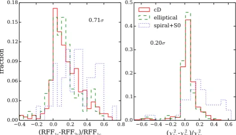
quan-titative information to assess whether BCGs are better fitted by a two-component model than by a one-component model, at least in very clear cases. Fig.9shows a comparison of these param-eters obtained for single-S´ersic and S´ersic+Exponential models. In the left-hand panel, we show a histogram of the fractional dif-ferences in the RFF values (RFF1c− RFF2c)/RFF1cfor all three
BCG types. The right-hand panel shows the correspondingχ2
ν
frac-tional differences (χ2
ν,1c−χ 2
ν,2c)/χ 2
ν,1c. It is clear that for disc BCGs,
the S´ersic+Exponential model does a better job. This is not sur-prising since spiral and lenticular galaxies contain clearly distinct bulges and discs. For elliptical BCGs, the improvement in RFF and χ2
ν for two-component models is generally quite small, as
expected: elliptical galaxies are known to be reasonably well fit-ted by S´ersic models, so the extra component does not improve the residuals significantly. Perhaps surprisingly, the improvement is also only marginally better for cDs: the typical fractional dif-ferences for cD galaxies are (RFF1c−RFF2c)/RFF1c=0.11+−00..1408
and (χ2
ν,1c−χ 2
ν,2c)/χ 2
ν,1c=0.035+ 0.053
−0.029(median+/−first and third
[image:10.595.48.285.528.664.2]quartiles of the parameter distributions).
Figure 9. Comparison of the residuals between single-S´ersic and S´ersic+Exponential models. The left-hand panel shows the fractional dif-ferences in RFF obtained with two-component and one-component fits for cD (red solid line), elliptical (green dashed line), and disc (blue dotted line) BCGs. The right-hand panel shows the corresponding fractional differences forχ2
ν.
Since the distributions shown in Fig.9for ellipticals and cDs are statistically indistinguishable, there is no clear separation that could be used to distinguish elliptical and cD BCGs by com-paring one-component and two-component fits. Moreover, on av-erage, S´ersic+Exponential model does not fit the profile of cD BCGs clearly better than single-S´ersic model. The reason is that for cD BCGs the values of RFF andχ2
ν are generally not
domi-nated by the presence or absence of a second exponential model component but by other structures present in the residual images, such as double cores. Since there is no clear improvement in the S´ersic+Exponential model, the model with the smallest number of parameters (i.e. single-S´ersic model) will be preferred for simplic-ity. The following discussions are based on the results from the single-S´ersic fits.
4.4 Summary of Section 4
In this section, we have analysed the differences in the structural properties of BCGs as a function of morphology. These structural parameters have been derived from one-component (S´ersic) and two-component (S´ersic+Exponential) model fits. Disc BCGs (a small minority) have smaller S´ersic indices (n) than elliptical and cD BCGs, as expected. They also have different, generally broader, distributions of RFF andχ2
ν. Elliptical and cD BCGs have similar
nvalues, but cDs tend to have larger values ofRe, RFF andχν2.
These differences do not depend strongly on whether we use one-or two-component models.
The observed structural differences could provide quantitative ways to separate elliptical and cD BCGs without relying on visual inspection. We explore these in Section 5. Furthermore, the differ-ences we have found in the structural parameters suggest that the formation histories of elliptical and cD BCGs may be different. For instance, gas-rich major mergers and other dissipative processes may be responsible for building the inner (S´ersic-like) component, while dissipationless minor mergers may contribute to the build-up of the outer extended envelope and to the growth of galaxy sizes (e.g. Oser et al.2010; Johansson et al.2012; Huang et al.2013). We will explore in a subsequent paper (Zhao et al., in preparation) whether the morphological and structural properties of BCGs are linked to other intrinsic BCG properties such as their stellar mass, and/or to the properties of their environment. These links will provide more clues to the formation history of cDs/BCGs.
5 S E PA R AT I N G E L L I P T I C A L A N D C D B C G s
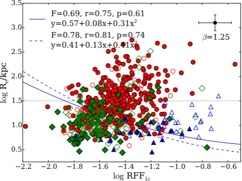
The results of Section 4.2 suggest that we may be able to use the different distributions of cD and non-cD BCGs on the logRe–
log RFF1cplane to separate them in an objective, quantitative and
automatic way. Fig.10shows that cDs are clearly segregated from other BCGs in this two-dimensional parameter space. We attempt to find a robust, well-defined way to separate, statistically, cD and non-cD BCGs using the information provided by this diagram. In other words, we suppose to find an ‘optimal border’ that can separate them.
5.1 Method description and the optimal border
Figure 10. logReversus log RFF1cfor the BCGs in our sample. We use this
diagram to find the optimal border to separate cD from non-cD BCGs. The symbols are the same as in Fig.4. The black dotted line is the ‘first guess’ for the border. The blue solid curve is the optimal border determined when we consider all cD BCGs (cD, cD/E and cD/S0) as cD galaxies. The blue dashed curve is the optimal border determined when we consider only pure cD and pure elliptical BCGs (excluding all cD/E, cD/S0, E/cD, E/S0, spiral and S0 BCGs). The legend shows the maximumF-score for the optimal borders and the corresponding completenessrand specificityp. The equations defining the optimal borders are also shown. The error bar shows the mean error of each parameter. We usedβ=1.25 in this case.
often results in a decrease in sample purity, and vice versa. We need therefore to find the best compromise between these competing requirements. In general, the optimal solution will depend on the specific intent for the selected sample, and therefore on the decision of how much weight to give to completeness and to purity. It is useful to define a measurement on the quality of the selection method that combines both requirements in a well-defined way. The optimal solution will then be obtained by maximizing this quality parameter. Following Hoyos et al. (2012) thesensitivity, which is often known ascompletenessin astronomy, is defined as
r= # True Positives
# True Positives+# False Negatives. (4)
Similarly, we definespecificityas
p= #True Negatives
# True Negatives+#False Positives. (5)
A ‘True Positive’ is an object retrieved by the selection process with the required properties (i.e. a cD galaxy that is correctly selected as such). A ‘False Negative’ is an item that is not retrieved by the selection process but does present the needed properties (a cD galaxy that is not selected). A ‘True Negative’ is an item that is rightfully rejected by the selection process since it does not have the required properties (for instance, an elliptical galaxy that is not selected as a cD). A ‘False Positive’ is an item that is incorrectly picked up by the selection process, but does not have the properties of interest (for example, an elliptical galaxy that is wrongly selected as a cD).
Sensitivityandspecificitycan be combined into a single number, known as the F-score (van Rijsbergen 1979), which provides a single measure on the quality of the selection process. TheF-score is just a weighted harmonic average ofrandp,
Fβ= (1+β
2)×p×t
β2×p+r , (6)
whereβis a control parameter that regulates the relative importance of completeness with respect to specificity. This is a user-supplied value that depends on the particular goals of the study. We will explore later how the choice ofβaffects our selecting results. At this stage, a value ofβ=1.25 is used, which can be thought of as weighing completeness more than the lack of contamination. For our BCG samples, theF-score is used to grade the performance of the diagnostics we use when separating cD galaxies from the parent population.
The selection process that we will apply to the parent popula-tion of BCGs in order to select cD galaxies will be defined by a ‘border’ in the logRe–log RFF1cplane (see Fig.10). This border
will be represented by a second-order polynomial in the horizontal coordinate. Higher-order polynomials (or more complex functions) could be used, but the additional complexity is not required here. In our specific problem, the cD galaxies play the role of the ‘items presenting the required properties’ discussed above, and the parent population is the complete sample of BCGs.
According to the definition ofsensitivityandspecificity, the BCGs in the parent sample are classified into four categories by their position relative to the border. In the logRe–log RFF1c plane, cD
galaxies dominate the region of largeReand RFF1c. We therefore
define this region as the ‘cD side’. Thus
(i) cD galaxies that fall on the cD side of the border are True Positives.
(ii) cD galaxies that do not fall on the cD side of the border are called False Negatives.
(iii) Elliptical and disc (spiral and S0) BCGs that fall on the cD side are regarded as False Positives.
(iv) Elliptical and disc (spiral and S0) BCGs that do not fall on the cD side of the border are True Negatives.
The optimal border is found by maximizing the F-score value. Following the method described in Hoyos et al. (2012), we use the Amoeba algorithm (Press & Spergel1988) to carry out this maximization and find the polynomial defining the border.
It is clear from Fig.10that the selected galaxy sample on the cD side of the optimal border will not contain only cD galaxies, and a degree of contamination will be present. We define contamination (Hoyos et al.2012) as
C= #non-cDs tested as positive
#all positives . (7)
The numerator are the non-cD BCGs which are on the cD side of the optimal border. The denominator of this fraction includes both cD galaxies and non-cD BCGs on the cD side.
Fig.10shows the logRe–log RFF1cplane for the BCGs in our
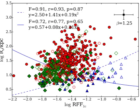
Figure 11. Two-step process to select cD BCGs. Symbols and legend are the same as in Fig.10. Disc (spiral and S0) BCGs are separated from non-disc BCGs (cDs and ellipticals) first using the optimal border shown as the blue dashed curve. cD galaxies are then selected using the optimal border shown as the blue solid curve. See the text for details.
this technique is more effective (cleaner) at selecting cD galaxies than at selecting non-cD BCGs.
Note that if we consider a ‘cleaner’ sample that contains only pure cD and pure elliptical BCGs (excluding all cD/E, cD/S0, E/cD, E/S0, spiral, and S0 BCGs), the optimal border (blue dashed curve in Fig.10) does not change significantly, but the quality of the selection as determined by theF-score value, the completenessr and the specificitypimproves. This is not surprising: the identification of BCGs as pure cDs/Es (as opposed to the ‘dubious’ ones) depends on more secure morphological characteristics which should be linked more clearly to the structural parameters. However, considering only this cleaner sample is not a realistic scenario since in practical cases we would like to start from a full sample of BCGs and find which ones are cDs. Nevertheless, it is reassuring that the border we determine does not depend very strongly on the exact training set used.
On the selected cD side, spiral BCGs are an important source of contamination. However, since most of them appear in the large RFF1cregion, it would be possible to go a step further to
imple-ment a simple further refineimple-ment in our method to separate spirals from the selected cDs: very few cD galaxies have log RFF1clarger
than∼−1.1. This would significantly improve the purity of the cD sample at very little cost in terms of its completeness.
Moreover, it is clear from Fig.10that all disc BCGs (spirals and S0s) contribute significantly to the contamination of either the cD or the elliptical samples separated by the best border. However, we can use the fact that disc BCGs distribute over a distinct area on the logRe–log RFF1cplane to apply a two-step process to exclude
them from our cD selection. First, the disc BCGs can be separated from the elliptical and cD BCGs, and then the cD BCGs can be selected out of the rest BCG sample. Fig.11illustrates the results of this two-step selection. The blue dashed curve is the optimal border determined in the first step. By excluding disc BCGs using this border, a very complete (r=0.93) and pure (p=0.87) non-disc BCG sample is built. The cDs can then be separated from the ellipticals using the optimal border shown by the blue solid curve with a completeness of 77 per cent (305 cDs are selected), and a contamination of only 14 per cent. Compared to the single-step cD selection (311 cDs were selected with 20 per cent contamination),
the two-step process clearly selects a very similar number of cDs but with better purity. The decision on whether the increase in purity is worth the additional complexity is left to the reader. In the reminder of this paper, we will use the single-step selection process for simplicity.
The automatic techniques we have developed can be applied to any BCG sample, but the optimal border needs to be adapted and calibrated using the imaging data from which the parent sample was derived. The calibration can be performed using a sub-sample of visually-classified BCGs, and then automatically applied to the complete sample using the structural parameters determined from standard single-S´ersic fits.
Aβvalue needs to be chosen depending on whether we are more interested in the completeness of the cD sample or in its purity, but we suggest thatβ=1.25 represents a reasonable compromise (see Section 5.3). Furthermore, it is important to remember that this method works better at selecting a sample of cD galaxies rather than a sample of non-cDs.
5.2 Distance to the optimal border
It is informative to explore the distribution of the points in the logRe–log RFF1cplane (Fig.10) in terms of their minimum
(per-pendicular) distance to the optimal border. We define the distance from each point to the optimal border as
D=
log RFF1c
σlog RFF1c
2
+
logRe
σlogRe
2
, (8)
wherelog RFF1cis the difference in log RFF1cbetween the data
point and the optimal border, and σlog RFF1c is the dispersion in
log RFF1ccomputed for all the points.logReandσlogRe have a
similar meaning but for logRe. Note that, because the units of the x- andy-axes are different, the distance is measured in units of the scatter of each parameter. For each point, the minimum distance
Dmincan be then determined. Fig.12shows the distribution of these
minimum distances for the different morphologies. As expected, the vast majority (>80 per cent) of the cDs show positive distances (they are above the optimal border line) while most of the ellipticals have negative ones. Under 20 per cent of the cDs spill over to the negative region, severely contaminating the non-cD sample, while a few ellipticals weakly contaminate the cD region. The measurement errors in logRe(∼0.16) and log RFF1c(∼0.13) result in distance
errors on the order of 0.7 in this metric. This contributes to the cDs’ ‘spillover’, but does not completely explain it. Reducing the measurement errors would certainly improve the performance of our method, but it would never make it perfect.
Interestingly, the spiral and S0 BCGs are quite well separated: the former show mostly positive distances while the later have mostly negative ones. This is mainly due to spirals having generally larger RFF1cvalues because the spiral arms and star-forming regions are
Figure 12. Distribution of the minimum distances to the optimal border shown in Fig.10for the cD and elliptical BCGs (top panel) and the spiral and S0 BCGs (bottom panel). Positive and negative distances correspond to points above and below the optimal border line, respectively.
the structural parameters: when the visual classifier is certain that a BCG is a cD, its structural parameters almost always confirm it, while in uncertain cases (e.g. cD/E) the structural parameters reflect this uncertainty. Similar conclusions can also be obtained from the pure elliptical BCGs and uncertain ones (e.g. E/cD), as shown in the bottom panel of Fig.13.
This analysis confirms the visual impression in terms of the BCG structure that there is a continuous distribution in the properties of the BCG extended envelopes, ranging from undetected (pure E class) to clearly detected (pure cD class), with the intermediate classes (E/cD and cD/E) showing increasing degrees of envelope presence. This continuous distribution in envelope detectability is reflected quantitatively in the structural parameters of the BCGs, by the minimum distance to the optimal border providing some indication of the relative importance of the envelope.
5.3 Effect of theβparameter
[image:13.595.54.277.64.451.2]In theF-score definition, theβparameter is used to apportion weight to the completeness and the specificity. For larger values ofβthe
Figure 13. Distribution of the minimum distances to the optimal border shown in Fig.10for the pure cD BCGs and cD/E BCGs (top panel). The bottom panel shows the corresponding histograms for pure E BCGs and E/cD BCGs.
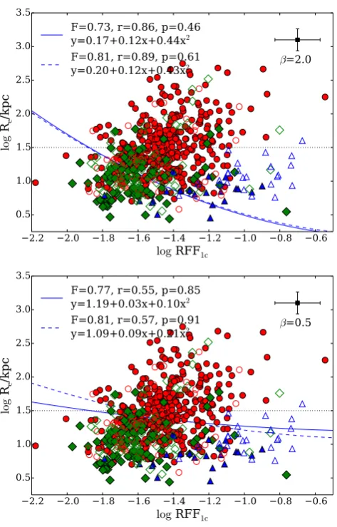
completeness is given a larger weight than the lack of contamination. Conversely, smaller values ofβ prioritise lack of contamination above completeness. To test how changingβaffects the results of the selection process, we repeat the exercise carried out in Section 5.1 but usingβ=2.0 andβ=0.5 in the determination of the optimal border.
Figure 14. Illustration of the effect ofβon the optimal border. The symbols, lines and legends have the same meaning as in Fig.10but we useβ=2.0 for the upper panel andβ=0.5 for the lower panel. Withβ=2.0 we give more weight to the completeness than to the lack of contamination. When usingβ=0.5, the lack of contamination is given more importance than achieving higher completeness. The choice onβdepends on the aims of the specific research.
technique is cleaner and more effective at selecting cD galaxies than at selecting non-cD BCGs.
As before, if we consider a cleaner sample that contains only pure cD and pure elliptical BCGs, the optimal border (blue dashed curve) does not change significantly, but the F-score value, the completenessrand the specificitypimprove. However, we have argued that this does not represent a realistic scenario.
We conclude thatβ=1.25 represents a good compromise, as its optimal border picks up a cD galaxy sample reasonably complete, and with relatively small contamination. However, no single value ofβcan be considered to be ‘correct’ and needs to be set according to the scientific goals of the study.
6 C O N C L U S I O N S
In this paper, we have analysed a well-defined sample of 625 low-redshift BCGs published inL07with the aim of linking their mor-phologies to their structural properties. We morphologically clas-sified the BCGs using SDSSr-band images and found that over half of them (∼57 per cent) are pure cD galaxies and pure
ellipti-cal BCGs constitute∼13 per cent of the sample. The intermediate classes (mostly cD/E or E/cD) account for∼21 per cent. It suggests a continuous distribution in the properties of the BCG extended en-velopes, ranging from undetected (pure E class) to clearly detected (pure cD class), with the intermediate classes (E/cD and cD/E) showing increasing degrees of envelope presence. We found this continuous distribution in envelope detectability is reflected quan-titatively in the structural parameters of the BCGs. There is also a minority of BCGs that are neither cD nor elliptical. About 7 per cent are disc galaxies (spirals and S0s, in similar proportions) and the rest (∼2 per cent) are in merging (see Appendix A).
In order to link the morphologies of the BCGs to their struc-tural properties, we have fitted the BCGs light distributions with the SDSSr-band images using one-component (S´ersic) and two-component (S´ersic+Exponential) models. We first characterized how well the models fit the target BCG by using two quantita-tive diagnostics. One diagnostic is the residual flux fraction (RFF), which measures the fraction of the galaxy flux presenting in the residual images after subtracting the models. The other diagnostic is the reducedχ2
ν. We concluded that generally it is very difficult
to find a robust diagnostic to decide, in a statistic way, whether a one-component or a two-component model is preferred for BCGs, especially for cD galaxies. Since there is no evident improvement by using two-component model fits, our other conclusions rely on the one-component S´ersic fits.
From simple one-component S´ersic profile fits, we have found a clear link between the BCGs morphologies and their structures, and claimed that a combination of the best-fitting parameters can be used to separate cD galaxies from non-cD BCGs. In particular, cDs and non-cDs show very different distributions in theRe–RFF1c
plane, whereRe is the effective radius and RFF1c is the residual
flux fraction, both determined from S´ersic fits. cDs have, generally, largerReand RFF1cvalues than ellipticals. Therefore we found, in
a statistically robust way, a boundary to separate cD and non-cD BCGs in this parameter space. BCGs with cD morphology can be selected with reasonably high completeness (∼75 per cent) and low contamination (∼20 per cent).
This automatic and objective technique can be applied to any current or future BCG samples which have good quality images. The method needs to be adapted and calibrated using the imaging data from which the parent sample was derived. Once calibrated with a representative sub-sample of visually-classified BCGs, this technique can be applied to the complete sample using the structural parameters determined from standard single-S´ersic fits.
In a subsequent paper (Zhao et al., in preparation), we will explore how the morphological and structural properties of BCGs are linked to other intrinsic BCG properties such as their stellar mass, and/or to the properties of their environments. These links will provide more clues to the formation history of cDs/BCGs.
AC K N OW L E D G E M E N T S