Probabilistic Cosmology

ISSN Online: 2153-120X ISSN Print: 2153-1196

DOI: 10.4236/jmp.2019.1012095 Oct. 30, 2019 1424 Journal of Modern Physics

Probabilistic Cosmology

Martin Tamm

Department of Mathematics, University of Stockholm, Stockholm, Sweden

Abstract

In this paper, an alternative approach to cosmology is discussed. Rather than starting from the field equations of general relativity, one can investigate the probability space of all possible universes and try to decide what kind of un-iverse is the most probable one. Here two quite different models for this probability space are presented: the combinatorial model and the random curvature model. In addition, it is briefly discussed how these models could be applied to explain two fundamental problems of cosmology: Time’s Arrow and the accelerating expansion.

Keywords

Cosmology, Ensemble, Time’s Arrow, Accelerating Expansion, Multiverse

1. Introduction

What is the most common way of solving a problem in physics? In the tradition which goes back at least to Newton, the dominating answer tends to be: Find the equations of motion (and solve them).

This answer has been enormously successful in the history of modern physics. This was also the way modern cosmology started a century ago. To illustrate this approach, let us consider a closed universe of the simplest possible topological type, i.e. a 4-sphere. And let us in addition also assume it to be homogeneous and isotropic at every moment of time. Can we then determine how the radius

( )

a t of the universe varies with time? The pioneering work for answering this question was based on the so called Friedmann equation (see Friedmann [1]):

( )

( )

( )

( )

0

2 2 3

6

6 d 6 _.

d

a a t

t

a t a t a t

 _{ + =}

 

  (1.1)

This is essentially just the time-time-component of Einstein’s general field equa-tions

How to cite this paper: Tamm, M. (2019) Probabilistic Cosmology. Journal of Mod-ern Physics, 10, 1424-1438.

https://doi.org/10.4236/jmp.2019.1012095

Received: September 30, 2019 Accepted: October 27, 2019 Published: October 30, 2019 Copyright © 2019 by author(s) and Scientific Research Publishing Inc. This work is licensed under the Creative Commons Attribution International License (CC BY 4.0).

http://creativecommons.org/licenses/by/4.0/

DOI: 10.4236/jmp.2019.1012095 1425 Journal of Modern Physics

8 ,

ij ij

G = πT (1.2)

where Gij is the Einstein tensor and Tij is the stress-energy tensor (for further

details, see e.g. Misner, Thorne, Wheeler [2] or Wald [3]). Multiplying by the factor a t

( )

( )

_{( )}

( )

_{( )}

d _{1 or} d _1,

d d

a a

a _t a _t

t a t t a t

 _{ = − = ± −}

 

  (1.3)

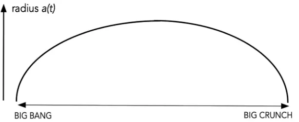
from which it is easy to see that a solution, starting from a=0 _{at the Big Bang,} will grow until it reaches its maximal value a0 and then, by symmetric consid-erations, decrease until it again becomes zero (at the Big Crunch). In fact, it is not difficult to see that the solutions of (1.3) are cycloidal curves, so the Fried-mann equation made it possible to predict the time-development of the universe from the beginning to the end (see Figure 1). Nowadays however, this is neither the best nor the most popular model for cosmology. In particular, it fails to ex-plain the accelerating expansion (see Adam, Riess et al. [4] and Perlmutter et al.

[5]).

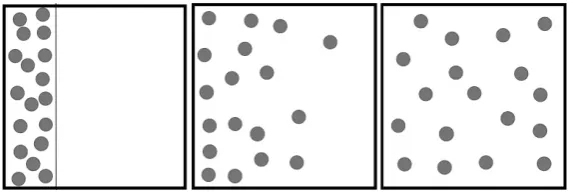
But, if we now return to the original question, there are also other answers to how problems in physics can be solved. For example, in statistical mechanics a competing answer could be: Consider all possibilities and find the most probable kind. As a trivial illustration, consider the situation where a gas is initially con-fined by a wall to a part of an otherwise empty container as in Figure 2 (left). What happens if the wall is removed? Clearly, the gas will immediately start to spread out (middle) to fill up the whole container, and at the end of this process (right), the gas will be very evenly distributed over the interior. How should we explain this phenomenon? It is of course in principle possible to try to use the

Figure 1. The time development of the closed Friedmann model.

DOI: 10.4236/jmp.2019.1012095 1426 Journal of Modern Physics equations of motion for some set of initial conditions. But this would lead to ex-tremely complicated computational problems, even for a moderate number of particles. A much simpler method, and in a sense a more convincing one, would be to note that the number of micro-states of the gas which correspond to the evenly distributed macro-state is enormously much larger than the number of micro-states which correspond to the un-evenly distributed macro-state we started with, and in fact much larger than the number of micro-states corres-ponding to any other macro-state as well. Thus, neglecting almost everything about the microscopic processes that underlies the development and instead just considering it to be more or less a random process, we can, using little more than high school mathematics, convincingly argue that the gas will end up in a state of even distribution.

The purpose of the present paper is to try to show how this way of reasoning could be used in modern cosmology, and also that it may have the potential to change our views on cosmology in general.

How should this way of thinking be implemented? The idea is to consider the set of all possible universes as a huge probability space, and then try to find out what types of universes dominate in this probability space.

It goes without saying that it is impossible to construct a model for the proba-bility space of all universes in any kind of detail. Rather, the strategy in this pa-per will be the opposite one; to find extremely simple models. Still, the hope is that these models will somehow reflect fundamental properties that are not so easy to spot within are more traditional framework.

Is this a multiverse theory? Answering this question will mainly be left to the reader, since it is more a question about philosophical interpretation than about science. From the specific point of view of the author however, the answer may be said to be yes: to consider all universes to have the same ontological status does seem to be the most natural interpretation. But on the other hand, it should be kept in mind that we are here concerned with multiverses of a very restricted kind, which can be viewed as a natural outflow of Feynmann’s “Democracy of all Histories” approach to physics. Thus, this is (regardless of the interpretation) essentially based on ordinary quantum physics and has no relation to the more speculative multiverse theories that have been discussed in recent years.

The main examples of such simplified multiverse models which I want to dis-cuss in this paper are the following:

• The combinatorial multiverse. • The random curvature multiverse.

DOI: 10.4236/jmp.2019.1012095 1427 Journal of Modern Physics

[6], Tamm [7], Tamm [8], Tamm [9]. The examples are as follows: • The asymmetry of time.

• The accelerating expansion.

It should also be said that the purpose here is not to make firm predictions to be compared to observations. Such predictions may very well be made at a later stage, but so far the ambition has rather been to make the models as simple as possible, and also they may contain various parameters which may be difficult to determine.

I will be mainly concerned with closed universes. Part of the reason for this will become clearer as we proceed. But it is of course possible to try to apply the same way of thinking to open universes as well. It is just harder to treat them in the context of probability spaces, something which is well known from ordinary quantum physics.

The underlying physics will mainly be treated in a kind of semi-classical set-ting. This is in a way very natural since the problems are macroscopic, but still in the end it may be argued that a quantum mechanical treatment would be pre-ferable. As has already been said, in this paper I consider simplicity in the pres-entation to be the most important thing. However, I will briefly come back to this question in Section 7.

2. The Combinatorial Multiverse

In this section we will study the perhaps simplest of all models, namely the com-binatorial one. Thus, for each moment of time between the endpoints −T0 and

0

T (corresponding to the Big Bang and the Big Crunch), consider the set of all possible configurations or “states” that a possible universe could be in. To simpl-ify still further, let us assume time to be discrete (and integer valued). Thus, we have moments of time

0, 0 1, 0 2, , 0 2, 0 1, ,0

T T T T T T

− − + − + _ − − _(2.1)

and for each such moment of time we have a certain number of possible states. At times −T0 and T0, we assume that there is only one unique state, but for each moment of time between the endpoints, there are many different states. All these states are then the nodes of a huge graph, and a universe is a path in this graph where the edges are specified by the dynamics of the model: between each pair of adjacent moments of time, say t and t+1, there will be a certain number of edges between the corresponding states, indicating those time-developments which are possible, and the totality of all such edges defines what we mean by the dynamics of the model. A very schematic picture is shown in Figure 3.

Remark 1. The word “state” here should be interpreted with some caution. It should not be interpreted as representing ordinary quantum states in the usual sense. Rather, states here may be thought of as “distinguishable configurations”, which is clearly a kind of semi-classical approximation (see Tamm [6]).

DOI: 10.4236/jmp.2019.1012095 1428 Journal of Modern Physics

Figure 3. One universe in the combinatorial multiverse [7].

example, the decay or non-decay of a certain particle may lead to completely different futures within a reasonably short time, in spite of the fact that the de-velopment of the underlying wave-function is supposed to be unique.

As it stands however, this model is too simple to generate any results. In fact, there are no observable differences at all between the states, which means that there are no measurable variables which could be related to the (so far non-specified) dynamics. In the next section, which is devoted to the second law of thermody-namics, we will therefore consider one additional variable: the entropy.

3. Time’s Arrow

The term “Time’s Arrow” was coined by Eddington [10] and refers to the fact that macroscopic time is directed; there is an arrow pointing from the past towards the future. For some reason we can remember yesterday but we cannot remem-ber tomorrow. Another formulation, which perhaps lends itself better to physi-cal reasoning, is to say that entropy grows in the direction towards the future.

The problem with Time’s Arrow is that the underlying equations of motion, which are supposed to be responsible for the macroscopic behavior, are essen-tially invariant under reversal of the direction of time. This can also be expressed by saying that on the microscopic level there is no arrow. So where does the ma-croscopic arrow come from?

There seems to be no question in physics where the tentative answers have been so diverse (see e.g. Barbour [11], Halliwell, Perez-Mercander, Zurek [12], Zeh [13]). One way to resolve this problem could be to simply just state that the boundary conditions of the universe are very different in the future and in the past. If we assume that the universe starts from a very improbable state of very low entropy immediately after the Big Bang, and then develops towards more and more probable states in the future very much like the gas in Figure 2, then the growth of entropy in between may appear to be perfectly natural, something which was in essence clear already to Ludwig Boltzmann. But assuming such differences in the boundary conditions would amount to little more than as-suming an arrow of time from the start.

DOI: 10.4236/jmp.2019.1012095 1429 Journal of Modern Physics would not at all imply that the time in each single universe would share this property. In fact, it could very well be that the symmetry would be broken so that the overwhelming majority of all universes would have a directed time, in the sense that the entropy would be monotonic. To put it shortly, all these un-iverses would have the same endpoints, but only half of them would have the same Big Bang as we have. In the other half, our Big Bang would instead be the Big Crunch.

To model this in a way which is sufficiently simple to allow for computations, we will make use of the combinatorial multiverse in the previous section, but with the concept of entropy added to it.

Thus, let us assume that to every state we can assign a certain number S which we call the entropy of the state. To make the model as simple as possible, let us also assume that S only takes integer values.

How many states correspond to a given value of S? According to Boltzmann, we have that

1

log S, e .kB

B

S k= Ω ⇔ Ω =W W = _(3.1) Although this formula was derived under special circumstances, it does represent a generally excepted truth in statistical mechanics: the number of states grows ex-ponentially with the entropy. In the following, this will be taken to hold true at every given moment of time for the universe as a whole. A schematic modifica-tion of Figure 3 for a very small multiverse is shown in Figure 4. In this picture, one possible path (universe) is shown, in this case with monotonically increasing entropy. However, before the model can be put into use we still need to specify which paths are allowed, i.e. specify the (time-symmetric) dynamics of the model. In other words, we need to agree on some rule for deciding which states are ac-cessible from a given state.

DOI: 10.4236/jmp.2019.1012095 1430 Journal of Modern Physics To this end, simplifying still further, we assume that the entropy can only change by ±1 during each unit of time. The idea is then to make use of Boltzmanns intuition that the universe with time moves from less probable states to more probable ones. In its original form however, this idea has a definite direction of time built in to it, which obviously makes it unsuitable in the present context. Therefore, we will instead make use of the following probabilistic time-symmetric version:

Principle 1. (The Time Symmetric Boltzmann Principle) For every state at time t with entropy S, the dynamics allows for a very large number K of “ access-ible states” with entropy S+1 _{at times} t−1 _and t+1_{. But on the other hand,} the chance δ _{for finding an edge leading to a state with entropy} S−1 _(at time t−1 _or t+1_{) is very small.}

Note that with this simplified dynamics, we do not compare the differences in probability between different paths in any detail. Rather, we just classify transi-tions as possible or not possible.

Remark 2. For the conditions in the symmetric Boltzmann principle to be compatible, it is necessary that K W, where W is the constant in (3.1). In fact, in this case it is easy to see that only a fraction K/W of states can be reached from states with lower entropy at the previous (or next) moment of time, so in this case, δ =K W _1_.

In addition to this, we also need some assumptions at the ends (BB and BC). In this case, let us assume that the entropy is zero, but that during the very first and last units of time, “everything is possible”, i.e. that there is a positive proba-bility for a transition to any of the states at the next (previous) moment. Howev-er, the probability does not necessarily have to be the same for all states. RathHowev-er, it seems very natural to assume that the probability for such a transition de-creases rapidly with the entropy of the state, i.e. the by far most probable transi-tions lead to states with very low entropy. This is of course just a coarse way of modeling the very extreme situation just after the Big Bang or just before the Big Crunch.

Summing up the discussion, we can now define the combinatorial multiverse with entropy added in the following way:

Definition 1. A universe U is a chain of states, one state Σt at time t for each

t, with the property that the transition between Σt and Σt′ is always possible according to the dynamical laws, where t′ = ±t 1.

Definition 2. The combinatorial multiverse (with entropy) M is the set of all possible universes U in the sense of Definition 1.

Note that with the above definitions, the probability weight of a certain un-iverse only depends on the weights of the first and last steps, since for all other steps we have simply put the weights equal to one.

4. The Broken Symmetry

DOI: 10.4236/jmp.2019.1012095 1431 Journal of Modern Physics universes with different kinds of behavior of the entropy, for this I simply refer to Tamm [6], Tamm [7], Tamm [8]. But it may still be worthwhile to briefly discuss how the combinatorial multiverse can be used to explain time asymme-try.

With suitable choices for the parameters of the model, it is easy to convince oneself that the probability for a universe with a monotonic behavior of the en-tropy is enormously much larger than, e.g. the probability for a universe with low entropy at both ends. In fact, if δ _{in the time symmetric Boltzmann}

prin-ciple is small enough, then the probability for such a behavior will be so small that it is almost neglectable in comparison with the probability for a monotonic behavior, even if in the monotonic case the last (or first) step will be very im-probable.

Thus, since it seems to be an experimental fact that we live in a universe with low entropy at least one end, we have in a sense arrived at an explanation for the fact that an observer who is confined to such a universe will, with overwhelming probability, experience a directed time: there are simply so many more universes of this kind.

Is this a sufficient explanation for the arrow of time? From the point of view of the author, this model should rather be considered as a first step towards such an explanation, and more refined models should be designed. Certainly, there are many simplifications in the above model, and some of them may even appear to be rather extreme. But on the other hand, most of them can be said to be quite harmless for explaining the underlying mechanism, e.g. discrete time and integ-er-valued entropy.

But there is one assumption which is somewhat problematic in the Symmetric Boltzmann Principle above: if we apply it probabilistically, then it leads to a kind of Markov property in the sense that the probability for the entropy to go up or down at a certain step is completely independent of the pre-history. This is quite in contrast to our own universe, where an event (e.g. a supernova), can leave traces that can still be seen billions of years later.

However, one can attempt to construct slightly more complicated models which do not have this behavior. For example, a kind of assumption which would not have this Markov property would be to assume that the probability for the increase/decrease of the entropy at a certain step (forwards or backwards in time) should depend on the n previous (following) steps. If we for instance let

2

n= , this would mean that an increase (or decrease) of the entropy from time

k

t to tk+1 will be more likely if we already know that at the previous step from 1

k

t − to tk the entropy has increased (decreased).

In fact, it can also be argued that such a modified model would not only be more realistic, but would also in a sense give clearer results than the above mod-el. For instance, one can attempt to prove that in such a model, the total proba-bility mass of all universes with directed time (in anyone of the two directions) must be very close to 1. And certainly, there are other ways to improve further.

DOI: 10.4236/jmp.2019.1012095 1432 Journal of Modern Physics or quantum mechanical mechanics is of course large. This is, for better or for worse, both the strength and the weakness of probabilistic cosmology as it is presented here: extreme simplification may be the price we have to pay in order to see the forest in spite of all the trees.

5. The Random Curvature Multiverse

In this section, we will briefly discuss another kind of simple model for a multi-verse, which is however quite different from the combinatorial multiverse in Sections 2, 3 and 4. Here it will not be the entropy but rather the scalar curvature which will be the central concept. Nevertheless, the basic approach is the same: we start from very general statistical assumptions and try to determine the most probable type of universe.

Thus, let us consider the probability space of all possible metrics on a certain space-time manifold, only subject to the condition that the total 4-volume is a fixed number. Scalar curvature is essentially additive in separate regions, so what can we say about the probability for a certain value of the total scalar curvature in a region D which is a union of many smaller regions?

Remark 3. It is generally believed that the fluctuations in R become more and more violent when we move towards shorter and shorter length scales. From this point of view, one can wonder if it makes sense to consider the total scalar cur-vature in a region at all?

The easiest way to get around this difficulty is to simply consider the mean scalar curvature at some (short) length scale. As it turns out, everything to come is essentially independent of the choice of this length scale, so I will not com-ment further on this here.

To each such smaller region we assume that there is a certain probability dis-tribution for the different possible metrics. Exactly what this probability distri-bution actually looks like on the microlevel is of course difficult to know, but the point is that under quite general assumptions this will not be important. Let us just suppose that it depends only on the scalar curvature. This is in fact very much in the spirit of the early theory of general relativity, where R plays a central role (compare e.g. the deduction of the field equations from the Hilbert Palatini principle in Misner, Thorne, Wheeler [2]). We also suppose, starting from the idea that zero curvature is the most natural state, that the mean value of this dis-tribution is zero. This assumption may be non-obvious, but nevertheless serves as a good starting point.

If we now consider the total curvature R in D to be the sum of the tions from all the smaller subregions, and if we (roughly) treat these contribu-tions as independent variables, then the central limit theorem (see Fischer [14]) says that the probability for a certain value of R is

{

}

exp −

µ

 (5.1)

where ∆ _{is the volume of D.}

DOI: 10.4236/jmp.2019.1012095 1433 Journal of Modern Physics the metric g in D on a macroscopic scale where we do not observe any fluctua-tions of the curvature. In other words, the factor in (5.1) can be considered as a kind of measure of the resistance of space-time against bending.

What about the probability weight of a larger set Ω =αDα with metric g? Assuming multiplicativity (which essentially means that different regions are treated as independent of each other), and that all the regions have roughly the same volume ∆, we get the (un-normalized) probability

( )

{

}

{

}

g g g

P α R_α R_α R V

α

µ_∆  µ_∆  µ _Ω

Ω Π − = _− _≈ −



∑

∫

 (5.2)

where µ _{is a fixed constant. (Here we have, in the transition from sum to}

integral, tacitly made use of the additive property of the variance in normal dis-tributions.) So what we get is a kind of Ensemble of all possible metrics in Ω_,

where each metric gets a probability weight as above.

In classical general relativity, R is usually assumed to be zero everywhere, as long as there is no mass present. This is of course very well compatible with the present Ensemble, since R=0 _{will obviously maximize the exponential in} (5.2). However, when it comes to cosmology things become more complicated, and this kind of Ensemble may lead to non-trivial consequences.

The word Ensemble originally steams from statistical mechanics. So the idea is now to apply methods from classical statistical mechanics to the whole multi-verse (see e.g. Huang [15] for some background about Ensembles). First

com-pute the “state sum”: _exp

{

}

g g ΩµR V

Ξ =

∑

_∫

state sum,  = −logΞ, is what is usually refered to as the “Helmholtz Free Energy”. According to standard wisdom in statistical mechanics, the macrostates which minimize  (among all states with a given volume), are the by far most probable ones, i.e. the ones which may be realized.

In general, finding these macrostates can be difficult, since they are deter-mined by a sensitive interplay between the size of the terms in the state sum and their corresponding “densities of state”. However, in the case of interest here, corresponding to low curvature, it can be a reasonable first order approximation to assume that the density of states is the same for all competing states. In this case,  can essentially be computed as minus the logarithm of the largest term in Ξ_:

2_{d .}

g

R V

µ

_∫

 (5.3)

Remark 4. Note that terms like the “Helmholtz Free Energy” are used here to associate to a fundamental statistical principle. But it should of course be kept in mind that in this situation we deal with 4-dimensional states, and that this is not directly related to ordinary 3-dimensional energy.

ac-DOI: 10.4236/jmp.2019.1012095 1434 Journal of Modern Physics tion.

What happens if we minimize the action/free energy  in the case of a closed, homogeneous, isotropic universe? (Compare with the closed Friedmann model in Section 1). As long as we consider an empty universe without mass, the answer will be just a four-sphere. In fact, it turns out that in Lorentz geometry, such a sphere has R=0 _{everywhere, which obviously makes it minimizing.}

Figure 5 looks rather similar to the closed Friedmann universe in Figure 1, but it is not exactly the same.

Just as in the case with the combinatorial multiverse without entropy, the model is so far too simple to be able to generate any interesting results. To make it more interesting, we need to also include matter. This will be initiated in the next section.

6. A Geometric Model for the Accelerating Expansion

Can probabilistic cosmology explain the accelerating expansion? (or more gen-erally, determine the scale factor, explain inflation etc.).

A commonly made implication of the accelerating expansion is that the un-iverse must be open. On the other hand, as has been pointed out in Section 1, probabilistic cosmology is most easily applied to closed universes, since there are problems with making the set of all open universes into a probability space. As it turns out however, this is not an issue in the present situation, since one of the conclusions is in fact that accelerating expansion may be a very natural pheno-menon also in closed universes. In this section, I will sketch a very simple model based on the random curvature multiverse of the previous section.

Let us now once more return to the closed, homogeneous, isotropic universe we started with in Section 1. If we accept the accelerating expansion as a reality, then the most common way of explaining it is to reinterpret the field equation, which leads to the idea of dark energy. But is it evident that the field equations are the right starting point?

An alternative approach is offered by probabilistic cosmology. As we saw in the previous section, the cosmology of an empty random curvature multiverse is rather simple. But if we also take into account matter, the situation becomes much more interesting. So how should the gravitational forces be included?

DOI: 10.4236/jmp.2019.1012095 1435 Journal of Modern Physics The easiest way, and also the most traditional one (although perhaps not the most fundamental one), is to actually continue the analogy between minimizing  and the principle of least action. In this case, we can simply add the ordinary action associated with gravitation to  to obtain the total action.

To make everything as easy as possible, let us just make use of the usual clas-sical concept of potential energy. In this case it is easy to see that the total gravi-tational energy at a certain moment of time t should be of the form

( )

a t

⋅ (6.1)

which then leads to a contribution to the total action:

( )

0 1 d ,

T

T _{a t} t

β ₋

−

_∫

for some constant β _.

Remark 5. The form of the expression in (6.1) of course just expresses the fact that the (negative) potential energy between two bodies is inversely proportional to their distance. From this it follows easily e.g. that an expanding homogeneous gas will behave exactly in this way.

However, our universe as we know it does not expand as a homogeneous gas. This may have been a reasonable picture during the very first part of our history. But for the present expansion, it is much better to imagine the expansion as tak-ing place in between galaxies of more or less fixed size and mass. This will still give rise to an expression like in (6.2) for the action, but possibly with quite a different value of β _{. The distribution of galaxies is by the way also an}

interest-ing field for probabilistic cosmology, but it would lead too far to go into this here.

This is one reason why the present model should not be expected to give ac-curate results near the endpoints. Another reason is that in this case, gravita-tional physics alone may not be enough to explain the expansion rate.

Summing up, the problems becomes to minimize

( )

0

2_d T 1 _d

T

R V t

a t

β

Ω −

Φ =

_∫

_∫

where Ω _{stands for the whole universe, under the condition that}

( )

V =

_∫

_∫

is a fixed number, corresponding to the total 4-volume of Ω_{. What do the}

solu-tions to this minimizing problem look like?

A traditional method of attack is to look at the Euler-Lagrange equation for the functional

( )

(

)

0

0

2_d T 1 _{d d .}

T

R V t V V

a t

λ _Ω β ₋ λ _Ω

Φ =

_∫

_∫

_∫

DOI: 10.4236/jmp.2019.1012095 1436 Journal of Modern Physics global minimum of Φ_{, even if condition (6.4) is satisfied, since there could also}

be other stationary solutions. As it turns out, there are strong indications that the solution in this case is unique, which would then imply that finding the global minimum is in this case equivalent to solving the Euler-Lagrange equa-tion. This is simply because the solutions to the equations in this paper tend to be uniquely determined (at least in the time-symmetric, homogeneous and iso-tropic case). But a rigorous treatment of this question leads to difficult and un-solved problems, which also require a much heavier mathematical machinery than I can go into here.

Having said this, we can still study the solutions to the Euler-Lagrange equa-tion on a time-interval corresponding to the main part of the time-span of each universe. An example is plotted in Figure 6. If we compare this plot with the one in Figure 5, we note that here there is an interval of time in the beginning of the development where the function a t

( )

Remark 6. It is quite a mathematical task to give a complete treatment of the minimizing problem in this section. Some more details are given in Tamm [9], but still a lot of work remains to be done.

However, it may be worthwhile to comment on the difference in underlying intuitive perspective between the classical theory and the present one.

In the classical closed Friedmann universe in Section 1, matter gives rise to an attractive force which makes the universe re-contract into a Big Crunch. From the intuitive point of view of a classical initial value problem, this makes the be-havior in Figure 1 very natural.

In the present context however, the perspective is somewhat different. Here the total volume is given from the start. Perhaps we may think of the universe as built up from a fixed number of elementary constituents of some kind, each with a fixed “elementary” volume. So how will the empty universe in Figure 5 react when we add mass? Clearly, the influence should still be contractive, and the contractive force should be strongest close to the endpoints. But since the vo-lume is fixed, contraction near the ends must imply expansion somewhere in between. From this point of view, the behavior in Figure 6 becomes very natu-ral.

DOI: 10.4236/jmp.2019.1012095 1437 Journal of Modern Physics Remark 7. As has already been stated, the above Lagrangian approach may be the easiest way to include mass in the model. But there are bolder alternatives. One can for instance conversely attempt to interpret gravitational action in terms of curvature instead. In fact, it can be argued that in general, the presence of mass implies non-zero scalar curvature, and thus that mass in itself will con-tribute to the scalar curvature. Moreover, it can also be seen that two interacting bodies will give rise to less curvature than the sum of their separate contribu-tions, in fact in a way similar to (6.2). This way of viewing the problem has the interesting property that in a sense it puts mass and the curvature of space-time on an equal footing: in both cases their influence on the physical development comes from their contributions to the integral

2_{d .} R V Ω

∫

7. Conclusions

The two examples in this paper both represent extremely simplified models for the multiverse, but they also represent two very different kinds of simplification. This is in fact one of the main reasons for choosing them as examples in this pa-per; to show that there are very different ways to implement probabilistic cos-mology.

But would it not be better to try to create a common model which could in-clude all aspects of probabilistic cosmology in a unified way? This would very much be like wishing for a grand unifying theory for all of fundamental physics: it would be wonderful to have one, but it is not obvious that we do ourselves a favor by advocating such a theory if the time is not ripe for it. From this point of view, the only reasonable way forward would seem to be to use different kinds of simplifications in different contexts, and only in the end we may hope that all these different aspects will unite into a more complete and unified picture.

Having said this, it is still worth pointing out that the best (at least in the opi-nion of the author) proxy to such a united approach that we have is Feynmann’s democracy of all histories approach to physics. And, at least from an abstract point of view, this approach seems to be very well suited for the use of probabil-istic cosmology. From a more applied point of view however, there may still be a long way to go before e.g. both the Combinatorial Multiverse and the Random Curvature Multiverse can be treated within such a common framework.

DOI: 10.4236/jmp.2019.1012095 1438 Journal of Modern Physics tool box, the better are the perspectives for a success.

Conflicts of Interest

The author declares no conflicts of interest regarding the publication of this pa-per.

References

[1] Friedmann, A. (1922) Zeitschrift fur Physik, 10, 377-386. https://doi.org/10.1007/BF01332580

[2] Misner, C.M., Thorne, K.S. and Wheeler, J.A. (1973) Gravitation. W. H. Freeman and Company, San Francisco.

[3] Wald, R.M. (1984) General Relativity. The University of Chicago Press, Chicago. https://doi.org/10.7208/chicago/9780226870373.001.0001

[4] Adam, G.R., et al. (1998) The Astronomical Journal, 116, 1009-1038. https://doi.org/10.1086/300499

[5] Perlmutter, S., et al. (1999) The Astronomical Journal, 517, 565-586. https://doi.org/10.1086/307221

[6] Tamm, M. (2013) Physics Essays, 26, 237-246. https://doi.org/10.4006/0836-1398-26.2.237

[7] Tamm, M. (2015) International Journal of Astronomy and Astrophysics, 5, 70-78. https://doi.org/10.4236/ijaa.2015.52010

[8] Tamm, M. (2016) Symmetry, 8, 11. https://doi.org/10.3390/sym8030011 [9] Tamm, M. (2015) Journal of Modern Physics, 6, 239-251.

https://doi.org/10.4236/jmp.2015.63029

[10] Eddington, A.S. (1928) The Nature of the Physical World. Cambridge University Press, Cambridge, Chapters 3 & 4. https://doi.org/10.5962/bhl.title.5859

[11] Barbour, J. (1999) The End of Time. University Press, Oxford.

[12] Halliwell, J.J., Perez-Mercander, J. and Zurek, W.H. (1994) Physical Origins of Time Asymmetry. Cambridge University Press, Cambridge.

[13] Zeh, H.D. (2001) The Physical Basis of the Direction of Time. 4th Edition, Springer Verlag, Berlin Heidelberg. https://doi.org/10.1007/978-3-540-38861-6

[14] Fischer, H. (2011) A History of the Central Limit Theorem: From Classical to Mod-ern Probability Theory, Sources and Studies in the History of Mathematics and Physical Sciences. Springer, New York.

https://doi.org/10.1007/978-0-387-87857-7_8