Analysis of Double and Single Sided Induction Heating Systems by Layer Theory Approach

(1)

doi:10.4236/jemaa.2010.27052 Published Online July 2010 (http://www.SciRP.org/journal/jemaa)

Analysis of Double and Single Sided Induction

Heating Systems by Layer Theory Approach

Layth Jameel Buni Qaseer

General & Theoretical Electrical Engineering Department, University of Duisburg-Essen, Duisburg, Germany. Email: [email protected]

Received February 11th_{, 2010; revised April 8}th_{, 2010; accepted April 15}th_{, 2010.}

ABSTRACT

The iterative layer theory approach is applied to the analysis of double sided and single sided induction heating systems for continuous heating of thin metal strips. The excitation is transverse to the direction of strip motion and can be three phase or single phase. Nonmagnetic as well as ferromagnetic strips are employed. The important system parameters, namely, strip resistance, reactance, induced power and electromagnetic force are introduced. Accuracy of the method is verified with measurement of practical induction heating system together with comparison to numerical and analytical methods.

Keywords:Eddy Currents, Electromagnetic Analysis, Energy Conversion, Induction Heating

1. Introduction

THREE phase induction heating systems such as transverse flux induction heating (TFIH) systems and traveling wave induction heating (TWIH) systems have been ex-tensively studied in recent years. While numerical tech-niques are more popular and particularly useful for in-vestigating the induced current and power distributions taking into account longitudinal and transverse edge ef-fects, analytical methods are more convenient for the integral parameters determination and analysis.

3-D finite element method (FEM) has been employed in the analysis of TFIH systems [1-8] while 2-D and 3-D FEM have been employed in the analysis of TWIH systems [9-13]. Few papers relating to analytical methods for the analysis of single phase and traveling wave but cylindrical induction heating systems have been published [14-17].

Only a few researchers pay attention to this area in the world.

The TWIH is not fully appreciated with respect to their main advantages and possible industrial applica-tions [18].

A. Ali, V. Bukanin from St. Petersburg Electrotechn- ical University in Russia and F. Dughiero, M. Frozen, S. Lupi, P. Siega, V. Nemkov from University of Padua in Italy have obtained significant achievements in this area. In the very recent years, Takamitsu Sekine, Hideo Tomita, Shuji Obata and Yokio Saito from Tokyo Den-

ki University in Japan have designed an excellent trav-eling wave induction heating system and carried out experiment [19].

An analytical method based on the decomposition of the main magnetic flux imposed by means of an excitation coil into partial magnetic fluxes along different regions that comprise the assembly. The basic circuit parameters that feature the electric performance in induction heating devices having an excitation axial winding as found in induction motors for generating rotary magnetic fields are mathematically modeled [20].

Modern analytical approaches using transmission line terminology [21-23] are confined to lossless or low conductivity (dielectric) media where displacement currents are prominent at microwave frequencies in the order of hundreds of gigahertz, which is not the case as in this approach where induced power is the major objective of induction heating, moreover these methods are primarily applied to isotropic media while the layer theory is applied to both isotropic and anisotropic media, also it is not mentioned in these references whether these approaches may be used in the case of three phase (traveling wave) excitation.

The layer theory approach has been mainly used for the analysis of linear, tubular linear and helical motion induction motors as given in [24-26].

(2)

pect to the long and thin continuously moving strip. Sin-gle sided induction heating (SSIH) systems are TWIH systems that employ one inductor for exciting the metal strip while single phase induction heating systems are commonly known as longitudinal flux induction heating (LFIH) systems.

The primary object of this paper is to propose a general mathematical model for the induction heating system using the actual topology for single phase and three phase excitations with any number of poles for SSIH and DSIH systems. As a second object, the paper employs the multi-layer approach with the appropriate current sheet to calculate the flux density components, induced power in the strip, terminal impedance and the magnetic force acting on the strip in the direction of field travel in the case of TWIH systems.

2. Mathematical Model

2.1 Three – Phase Excitation

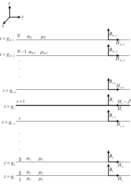
A general multi-region problem is analyzed. Figure 1

shows a cross-section of the N-region model used in the theory. The model is taken to be a set of planar regions. The current sheet lies between regions r and r + 1.

. . .

1

N N1 N1

N _N N

1

N

H _

2

N

H 

1

r

H

r

H

r

H J 1

N

B 

2

N

B 

1

r

B_

r

B x

y z

. . .

r

z g 1

r

z g 

1

r

1

 1

1 2

 2

2 3

 3

3

1 z g

2 H

1 H 2 B

1 B 2

z g

1

r

B

1

r

H

r 1

r

z g _ 2

N

z g 

1

N

z g 

σ1 μ1

σ3 μ3

σ2 μ2

σN-1 μN-1

[image:2.595.59.286.375.694.2]

σN μN

Figure 1. General model with current sheet at boundary

r z = g

The current sheet varies sinusoidally in the y-direction and with time. It is of infinite extent in the x-direction and infinitesimally thin in the z-direction.

Regions 1-N are layers of materials where the general region n has a conductivity σn and anisotropic relative

permeability µn. The anisotropy is an approximation

made in order to deal with slotted regions. The regions are traveling at velocity (1sn)f relative to a

station-ary reference frame where λ is the wavelength of applied field, f is the frequency and snis the slip in region n

de-fined as

n n

f s

f



where fn is frequency of the field experienced by region n.

In this frame the traveling field has a velocity f . It is assumed that displacement current is negligible and magnetic saturation is neglected. Maxwell’s equations for any region in the model are

H J

 

(1)

B E

t     



(2)

0

B

   (3)

0

E

   (4)

J E (5)

BH (6) The boundary conditions may be summarized as follows

1) The normal component of the magnetic flux density

Bz is continuous across a boundary.

2) All field components vanish at

z

 

.

3) The tangential component of magnetic field strength Hy is continuous across a boundary, but allowance

must be made for the current sheet in the manner ex-plained in Section 3.

2.1.1 Excitation Current Density

It is assumed that the winding produces perfect sinusoi-dal traveling wave. The line current density may be rep-resented as





Re exp[ ( )]

J  J j t ky  (7)

where J , and k are the line current density, angular frequency and wave length factor respectively. The line current density is given by

6 2N Ieff J

p

  

where I, p, τ and Neff are the r.m.s. value of the phase

(3)

of series turns per phase respectively. The wave length factor is defined as

k

 

 (8)

2.1.2 Field Equation of a General Region

As a first step in the analysis the field components of a general region are derived, assuming that all fields vary as exp[j(ωt – ky)], and omitting this factor for simplicity reasons from all the field expressions that follow. Taking only the x- component from both sides of (2) yields

0 x

B 

From (3) we have

z y B

jkB z

 _ 

which leads to

2

y

z B

B jk

z z

 

 

 (9)

Taking the z- component from both sides of (2) yields

x z

E B

k



  (10)

Taking only the x-component from both sides of (1) yields

y z

x B

B

E

y z 

 

 

  (11)

Therefore, using (9) and (10) into (11) yields 2

2 2

z Z B

α B

z 



 (12)

where

2 2

0 r

α k  jωμ μ σ

The solution is given by

cosh( ) sinh( )

z

B A αz C αz (13) where A and C are arbitrary constants to be determined from the boundary conditions.

From (3) we get





0

sinh( ) cosh( )

y

r

α

H A αz C αz

jkμ μ

  (14)

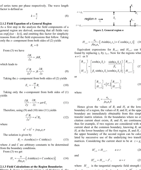
[image:3.595.56.533.72.648.2] [image:3.595.291.541.86.524.2]

2.1.3 Field Calculations at the Region Boundaries Figure 2 shows a general region n of thickness Sn the

normal component of magnetic flux density on the lower boundary is Bn-1 and the tangential component of mag-netic field strength is Hn-1. The corresponding values on the upper boundary are Bn andHn. From (13) and (14)

, cosh( ) sinh( )

z n n n n n

B A α z C α z (15)

1

n

zg

n

H

1

n

H_

n

B

1

n

B_

n

zg

n S

region n

n

f

Figure 2. General region n





, 0

sinh( ) cosh( )

n

y n n n n n

n

α

H A α z C α z

jkμ μ

  (16)

Equivalent expressions for Bz,n-1 and Hz,n-1 can be found by replacing znby zn-1. Now for the regions where

1

n or N

, , 1

cosh( ) sinh( )

z n n n n n z n

n

n n

y n n n n y n

B α S α S B

β

α S

H β αS H



     

 _ _ 

     

  _ _  

   

(17)

or

 

, , 1

z n z n

n

y n y n

B B

T

H H



   



   

    (18)

where

0

n n

n

α β

jμ μ k

 (19)

Hence given the values of Bz and Hy at the lower

boundary of a region, the values of Bz and Hy at the upper

boundary are immediately obtainable from this simple transfer matrix relation. At the boundaries where no ex-citation current sheet exists, Bz and Hy are continuous;

thus for example, if two regions are considered with no current sheet at the common boundary, knowing Bz and Hy at the lower boundary of the first region, Bz and Hy at

the upper boundary of the second region can be calcu-lated by successive use of the underlying two transfer matrices. Considering the current sheet to be at zgr,

then

, ,

y n y n

H H , n r (20) and

, ,

y n y n

H H J, n r (21) where H_{y n}_, is the tangential magnetic field strength in close lower proximity to the boundary and Hz n, is the

tangential magnetic field strength in close upper prox-imity to the boundary.

(4)

  



, 1 1 2 , 1 z n n n y n B T T H             …

 

, 1 , z r r y r B T H J      _ _

  (22)

and an inner part which supports the following relation

   

, 1 , z r r r y r B T T H          …

 

,1 2 ,1 z y B T H     

  (23)

If the top region is now considered, then as z , tanh( )αz 1 and all field quantities tend to zero, hence on the boundary gN1 the field quantities are related by

1 1

N N N

H _  β B _ (24) Therefore at any z within region N the field quantities become









1exp 1

z N N N

B B _ α g _ z

1exp{ ( 1 )}

y N N N N

H  β B _ α g _ z

Considering the bottom region where n= 1, the field quantities are related by

1 1 1

H βB (25) and at any z within region 1









1exp 1 1

z

B B α z g

1 1exp{ (1 1)}

y

H βB α z g

2.1.4 Surface Impedance Calculations

The surface impedance looking outwards at a boundary of zgn is defined as

, ,

1

, ,

x n z n n

y n y n

E B

Z

H k H



  _   _ (26)

and the surface impedance looking inwards is defined as

, ,

x n z n n

y n y n

E B

Z

H k H



   (27)

Using the method obtained in [17] with the values of

Bz,N-1, Hy,N-1, Bz,1, Hy,1 and [Tn]as derived in the previous

sectionthen 1 1 r r in r r Z Z Z Z Z    

 (28)

where Zin is the input surface impedance at the current

sheet and Zr+1and Zr are the surface impedances looking

outwards and inwards at the current sheet. Substituting for Zr and Zr+1 using (26) and (27) respectively, and re-arranging the terms yields

,

, ,

x r in

y r y r E Z

H H

 



 (29)

Substituting (21) into (29) yields

, x r in E Z J  

 (30)

Thus the input surface impedance at the current sheet has been determined. This means that all field compo-nents can be found by making use of this and (27), (22), (23).

2.1.5 Terminal Impedance, Power and Tangential Force

The terminal impedance per phase per metre of axial length can be derived [17] in terms of Zinas

2 24 eff t in N Z Z λp

 Ω/m (31)

Having found Ex, Bzand Hy at all boundaries, it is then

a simple matter to calculate the power entering a region through the concept of Poynting vector. The time average power density passing through a surface is given by



*



1 Re 2

P  E H W/m2

Hence the time average power density flowing up-wards from the current sheet at zgr is given by



*



, , ,

1 Re 2

in r x r y r

P  E H

and the time average power density flowing downwards from the current sheet at zgr is given by



*



, , ,

1 Re 2

in r x r y r

P   E H

The net power density in a region is the difference between the power in and power out



* *



, , , ,

Re 2

in z r y r z r y r

ω

P B H B H

k 

   (32)

It follows that the tangential force density Fy acting on

the strip is the net power density induced divided by traveling wave velocity λf

in y

P F

λf

 N/m2₍₃₃₎

2.1.5.1 Single Phase Excitation

(5)

Re{ exp( )}

J J jωt (34) with

1

2

J  N I

In this case k0, all field relations, Maxwell’s equa-tions and boundary condiequa-tions hold. The solution is given by

cosh( ) sinh( )

z

B A αz C αz (35) where

2

0 r

α  jωμ μ σ (36)

If the plane z0 passes through the central axis of the strip then

/ 2 cosh( / 2) sinh( / 2)

b

B A αb C αb

where b is the thickness of the strip and Bb/ 2 is the axial (tangential) component of magnetic flux density at the upper surface of the strip. The axial component of mag-netic flux density at the lower surface of the strip is given by

/ 2 cosh( / 2) sinh( / 2)

b

B A αb C αb

Hence we can write

/ 2 / 2 0cosh( / 2)

b b

B B B αb (37)

where B0 is the axial component of magnetic flux density at the centre of the strip.

The input surface impedance at the current sheet be-comes

in r

Z Z (38) where Zris obtained using (27).

The net power density induced in the strip is obtained using the concept of Poynting vector and therefore the net power density in the strip is

* *

, 1 , 1 , ,

2

2 1

Re{ }

2

Re{ tanh( / 2)}

in x n y n x n y n

P E H E H

J

α αb w m

σ

 

 

 

(39)

The terminal impedance is given by the relationship

tanh( / 2)

t α

Z αb

σ

 (40)

3. Numerical Results

The solution procedure that has been described in the previous sections is used to analyze two examples to check validity and accuracy. One example is a single phase practical induction heating system with ferromagnetic strip [27]. The importance of this example is that meas-urement is available in addition to calculation. The other

example is based on FEM solution for DSIH system [9]. For comparison reasons, FEM computation is adopted in our analysis which is widely used as a numerical tech-nique for this kind of applications.

In our implementation, the field domain is divided into a number of regions, each being defined by its coordi-nates, permeability and conductivity. Each region is de-scritized using first order triangular elements [28]. The induced power in the strip is obtained through the solu-tion of governing differential equasolu-tion for each nodal magnetic vector potential. Three values of power are computed: the power integrated over the coil, the air gap power and the power integrated over the strip.

The solution is assumed to be convergent when these three values do not differ by more than 1% which is termed as the power mismatch or power imbalance.

3.1 Practical Single Phase Induction Heating System

[image:5.595.310.538.429.552.2]

Problem data are given in Table 1. Results obtained us-ing the layer theory approach and FEM are in good agreement with measurement as shown in Table 2. This agreement is attributed to the fact that strip thickness is very small compared to strip length and width which coincides with the assumptions made in the mathematical model.

Table 1. Problem data for practical induction heating sys-tem (based on [27], Ex. 13)

Strip thickness, (mm) 1.56 Strip width, (mm) 1220 Strip length, (mm) 1270 Relative permeability of strip 50 Mean strip conductivity, (S/m) 1.333 × 106

Production rate, (ton/hr) 9.072 Heat cycle, (sec) 7.5 Speed of strip, (m/s) 0.169 Frequency, (Hz) 9600 Coil axial length, (mm) 1270 Coil width, (mm) 1270 Air gap length, (mm) 73.32 Amplitude of line current density, (kA/m) 31.831

Table 2. Computed parameters of the practical single phase induction heating system

Parameter _{value [18]}Measured

Value calculated by empirical formula [18]

FEM

Layer theory value

Strip power

(kW) 1490 1856.3 1824.9 1903.9

Strip resistance

(Ω) — 1.86 1.82 1.9 Reactance

[image:5.595.310.537.596.716.2]

(6)

Figure 3 shows the variation of the axial component of magnetic flux density along strip depth at mid coil axial length for single phase model using FEM analysis and the layer theory approach. The agreement between the results of both methods may be considered good with a maximum relative deviation of 4.9%. It is shown in this figure that the axial component of magnetic flux density decreases rapidly (exponentially) from the surface of the strip for both sides due to skin effect. Obviously there is no normal component for single phase induction heating system and this can be derived directly from Maxwell’s equations.

3.2 Single Sided and Double Sided Traveling Wave Induction Heating Systems

Reference [9] employed a double sided induction heating system whose data are given in Table 3.

-0.8 -0.6 -0.4 -0.2 0 0.2 0.4 0.6 0.8 1.1

1.2 1.3 1.4 1.5 1.6 1.7 1.8 1.9 2

Strip Depth (mm)

A

xial

F

lu

x D

e

ns

ity

(

T

)

layer theory finite element layer theory finite element layer theory finite element layer theory finite element

Central axial plane of strip

Figure 3. Variation of axial flux density component with strip depth for single phase induction heating model

Table 3. Problem data for traveling wave DSIH and SSIH systems (based on Reference [9])

Strip thickness, (mm) 2 Strip width, (mm) 1000 Strip length, (mm) 960 Relative permeability of strip 1 Mean strip conductivity, (S/m) 3.03 × 107

Axial pole pitch, (mm) 480 Slot pitch, (mm) 160 Slot width, (mm) 80 Slot depth, (mm) 40 Slots per pole per phase 1 Number of axial poles 2 Number of conductors per slot 8

Frequency, (Hz) 50

Inductor axial length, (mm) 960 Inductor width, (mm) 1000 Magnetic yoke depth, (mm) 80 Air gap length between yoke & strip, (mm) 15 Amplitude of line current density, (kA/m) 200 Input phase voltage, (V) 220

For the sake of comparison, the same model is adopted as a single sided induction heating system using the same line current density by removing one of the inductors along with its backing iron. Table 4 shows the computed parameters for both systems using FEM and the layer theory approach. Again the results correlate well as dis-cussed in Subsection 3.1.

Figure 4 and Figure 5 show respectively the variation of normal and tangential (axial) flux density components along magnetic gap length. The maximum deviation be-tween the results of both methods is found to be 5.2%.

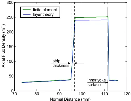
Figure 6 and Figure 7 show the variation of normal and tangential (axial) flux density components along dis-tance normal to the strip. Again both methods correlate well within 4%. In both systems the axial flux density component in the air gap is greater than the normal component, this may be attributed to the fact that the pole pitch is much greater than the air gap length in both sys-tems and in this case these syssys-tems are considered as axial flux machines. It is clear from these figures that the axial component of magnetic flux density is decreased within the strip due to skin effect which is not effectively pronounced in the normal component to the strip.

Table 4. Computed parameters for traveling wave induc-tion heating systems

Parameter _ValueFEM Layer Theory_Value

Per phase DSIH strip resistance (Ω) 0.0497 0.0513 Per phase DSIH reactance (Ω) 0.014 0.017 DSIH strip power (kW) 1210.3 1250.2

DSIH axial force (N) 23914.5 26045.3 Per phase SSIH strip resistance (Ω) 0.0125 0.012 Per phase SSIH reactance (Ω) 0.0087 0.0086 SSIH strip power (kW) 305.06 292.8

SSIH axial force (N) 6300 6099.9

70 80 90 100 110 120 130 115

120 125 130 135 140 145

Normal Distance (mm)

No

rm

a

l Fl

ux

De

n

si

ty

(

m

T)

layer theory finite element magnetic gap

(7)

70 80 90 100 110 120 130 0

50 100 150 200 250 300

A

xial

F

lux

D

e

ns

ity

(

m

T

)

layer theory finite element strip

thickness

[image:7.595.63.281.82.247.2]

magnetic gap

Figure 5. Variation of axial flux density component along normal distance to strip for double sided induction heating system

finite element layer theory

70 80 90 100 110 120

0 10 20 30 40 50 60 70 80 90 100

N

o

rm

a

l F

lux

D

e

ns

ity

(

m

T

)

finite element layer theory finite element layer theory finite element layer theory

strip thickness

[image:7.595.64.282.304.465.2]

inner yoke surface

Figure 6. Variation of normal flux density component along normal distance to strip for single sided induction heating system

70 80 90 100 110 120

0 50 100 150 200 250 300

A

xi

a

l F

lux

D

ens

ity

(

m

T

)

finite element layer theory finite element layer theory finite element layer theory

inner yoke surface strip

thickness

Figure 7. Variation of axial flux density component along normal distance to strip for single sided induction heating system

4. Conclusions

The layer theory approach has been used for the analysis of single sided, double sided traveling wave and single phase induction heating systems. This method has been applied to compute electrical parameters of various in-duction heating systems with ferromagnetic and non-magnetic thin strips.

The results show clearly that the theoretical results correlate well with finite element method results in addition to experimental one. This may be considered as fair jus-tification to the analysis method proposed in this paper.

5. Acknowledgements

The author is deeply indebted to Professor Daniel Erni, his host and co-worker at the University of Duisburg-Es- sen for advice and encouragement.

REFERENCES

[1] F. Dughiero, M. Forzan and S. Lupi, “3-D Solution of Electromagnetic and Thermal Coupled Field Problems in the Continuous Transverse Flux Heating of Metal Strips,”

IEEE Transactions on Magnetics, Vol. 33, No. 2, 1997,

pp. 2147-2150.

[2] V. Bukanin, F. Dughiero, S. Lupi, V.Nemkov and P. Siega, “3D-FEM Simulation of Transverse-Flux Induction Heat-ers,” IEEE Transactions on Magnetics, Vol. 31, No. 3, 1995, pp. 2174-2177.

[3] F. Dughiero, M. Forzan, S.Lupi and M. Tasca, “Numeri-cal and Experimental Analysis of an Electro-Thermal Coupled Problem for Transverse Flux Induction Heating Equipment,” IEEE Transactions on Magnetics, Vol. 34, No. 5, 1998, pp. 3106-3109.

[4] N. Bianchi and F. Dughiero, “Optimal Design Techniques Applied to Transverse-Flux Induction Heating Systems,”

pp. 1992-1995.

[5] Z. Wang, X. Yang, Y. Wang, and W. Yan, “Eddy Current and Temperature Field Computation in Transverse Flux Induction Heating Equipment for Galvanizing Line,”

pp. 3437-3439.

[6] Z. Wang, W. Huang, W. Jia, Q. Zhao, Y. Wang and W. Yan, “3-D Multifields FEM Computations of Transverse Flux Induction Heating for Moving Strips,” IEEE

Trans-actions on Magnetics, Vol. 35, No. 3, 1999, pp. 1642-

1645.

[7] D. Schulze and Z. Wang, “Developing an Universal TFIH Equipment Using 3D Eddy Current Field Computation,”

pp. 1609-1612.

[8] S. Galunin, M. Zlobina and K. Blinov, “Numerical Model Approaches for In-Line Strip Induction Heating,”

Pro-ceedings of 2009 IEEE EUROCON Conference, Saint-

[image:7.595.67.277.520.681.2]

(8)

[9] F. Dughiero, S.Lupi, V. Nemkov and P. Siega, “Travel-ling Wave Inductors for the Continuous Induction Heat-ing of Metal Strips,” Proceedings of 7th Mediterranean

Electrotechnical Conference, Antalya, 12-14 April 1994,

pp. 1154-1157.

[10] L. L. Pang, Y. H. Wang and T. G. Chen, “Analysis of Eddy Current Density Distribution in Slotless Traveling Wave Inductor,” Proceedings of 2008 International

Con-ference on Electrical Machines and Systems, Wuhan, 17-

20 October 2008, pp. 472-474.

[11] S. Lupi, M. Forzan, F. Dughiero and A. Zenkov, “Com- parison of Edge-Effects of Transverse Flux and Traveling Wave Induction Heating Inductors,” IEEE Transactions

on Magnetics, Vol. 35, No. 5, 1999, pp. 3556-3558.

[12] Y. Wang and J. Wang, “The Study of Two Novel Induc-tion Heating Technology,” Proceedings of 2008

Interna-tional Conference on Electrical Machines and Systems,

Wuhan, 17-20 October 2008, pp. 572-574.

[13] S. Ho, J. Wang, W. Fu and Y. Wang, “A Novel Crossed Traveling Wave Induction Heating System and Finite Element Analysis of Eddy Current and Temperature Dis-tributions,” IEEE Transactions on Magnetics, Vol. 45, No. 10, 2009, pp. 4777-4780.

[14] F. Dughiero, S. Lupi and P. Siega, “Analytical Calcula-tion of Traveling Wave InducCalcula-tion Heating Systems,”

Pro-ceedings of 1993 International Symposium on

Electro-magnetic Fields in Electrical Engineering, Warsaw, 1993,

pp. 207-210.

[15] V. Vadher and I. Smith, “Traveling Wave Induction Heat-ers with Compensating Windings,” Proceedings of 1993

International Symposium on Electromagnetic Fields in

Electrical Engineering, Warsaw, 1993, pp. 211-214.

[16] A. Ali, V. Bukanin, F. Dughiero, S. Lupi, V. Nemkov and P. Siega, “Simulation of Multiphase Induction Heating Systems,” Proceedings of 2nd International Conference

onComputation in Electromagnetics, Nottingham, 12-14

April 1994,pp. 211-214.

[17] L. Bunni and K. Altaii, “The Layer Theory Approach Applied to Induction Heating Systems with Rotational Symmetry,” Proceedings of 2007 IEEE Southeast

Con-ference, Richmond, 22-25 March 2007, pp. 413-420.

[18] L. L. Pang, Y. H. Wang and T. G. Chen, “New

Develop-ment of Traveling Wave Induction Heating,” IEEE

Trans-actions on Applied Superconductivity, Vol. 20, No. 3,

2010, pp. 1013-1016.

[19] T. Sekine, H. Tomita, S. Obata and Y. Saito, “An Induc-tion Heating Method with Traveling Magnetic Field for Long Structure Metal,” Electrical Engineering in Japan, Vol. 168, No. 4, 2009, pp. 32-39.

[20] E. Carrillo, M. Barron and J. Gonzalez, “Modeling of the Circuit Parameters of an Induction Device for Heating of a Non-Magnetic Conducting Cylinder by Means of a Traveling Wave as an Excitation Source,” in Proceedings

of 2nd International Conference on Electrical &

Elec-tronics Engineering, Mexico City, 7-9 September 2005,

pp. 258-261.

[21] X. M. Yang, T. J. Cui and Q. Cheng, “Circuit Represen-tation of Isotropic Chiral Media,” IEEE Transactions on

Antennas & Propagation, Vol. 55, No. 10, 2007, pp. 2754-

2760.

[22] A. C. Boucouvalas, “Wave Propagation in Biaxial Planar Waveguides Using Equivalent Circuit in Laplace Space,”

Proceedings of 1995 UK Performance Engineering of

Computer & Telecommunication Systems, Liverpool, 5-6

September 1995, pp. 258-266.

[23] H. Oraizi and M. Afsahi, “Analysis of Planar Dielectric Multilayers as FSS by Transmission Line Transfer Matrix Method (TLTMM),” Progress in Electromagnetics Re-

search, Vol. 74, 2007, pp. 217-240.

[24] E. M. Freeman, “Traveling Waves in Induction Machines: Input Impedance and Equivalent Circuits,” IEE Proceed-ings, Vol. 115, No. 12, 1968, pp. 1772-1776.

[25] E. M. Freeman and B. E. Smith, “Surface Impedance Me- thod Applied to Multilayer Cylindrical Induction Devices with Circumferential Exciting Currents,” IEE Proceed-ings, Vol. 117, No. 10, 1970, pp. 2012-2013.

[26] J. H. Alwash, A. D. Mohssen and A. S. Abdi, “Helical Motion Tubular Induction Motor,” IEEE Transactions on

Energy Conversion, Vol. 18, No. 3, 2003, pp. 362-396.

[27] N. R. Stansel, “Induction Heating,” McGraw-Hill, New York, 1949.