Portfolio Selection in Mean Minimum Return Level Expected Bounded First Passage Time Framework

(1)

ISSN Print: 2162-2434

DOI: 10.4236/jmf.2019.93012 Jun. 20, 2019 229 Journal of Mathematical Finance

Portfolio Selection in Mean-Minimum Return

Level-Expected Bounded First Passage Time

Framework

Tsotne Kutalia

Georgian American University, Tbilisi, Georgia

Abstract

This paper explores the selection of optimal portfolio by replacing the stan-dard Mean-Variance model by Mean-Minimum Return Level (MRL) frame-work and adding one important dimension—expectation of bounded First Passage Time (FPT) towards the MRL. To measure how much a given portfo-lio is exposed to risk, the new model can capture both, the amount of the largest possible loss at a certain confidence level and time to such an event occurring. The novelty of this paper is the introduction of bounded first pas-sage time towards MRL and taking its expectation into consideration as an additional factor in portfolio selection decision making. Assuming that the asset price dynamics follow multi-dimensional Geometric Brownian Motion with drift, we obtain a portfolio wealth process for multiple assets and we evaluate the lowest possible value to which it can drop by a high confidence level. Then we extend our examination of the optimal portfolio selection by ultimately obtaining the efficient surface of risky portfolios. As a result, the paper shows that the third dimension can make a significant difference while choosing the asset weights compared to classical models ignoring the portfo-lio return paths as long as they achieve a desired combination of risk and re-turn.

Keywords

Multi-Dimensional Geometric Brownian Motion, Ito’s Process, Portfolio Optimization, Optimal Stopping Time

1. Introduction

Portfolio selection theories have gone through various improvements since the introduction of its most prominent theory by Harry Markowitz in 1952. He was

How to cite this paper: Kutalia, T. (2019) Level-Expected Bounded First Passage Time Framework. Journal of Mathematical Finance, 9, 229-238.

https://doi.org/10.4236/jmf.2019.93012

Received: May 13, 2019 Accepted: June 17, 2019 Published: June 20, 2019

http://creativecommons.org/licenses/by/4.0/

(2)

DOI: 10.4236/jmf.2019.93012 230 Journal of Mathematical Finance

first to introduce the risk-return principle with the well-known Mean-Variance framework. The basic idea is to arrive at an efficient frontier curve of risky assets by minimizing volatility for given expected returns. It is shown that taking more than one risky position can eliminate some portion of risk as an investor realizes the effect of diversification. Volatility as a risk measure is ideal when portfolio returns are normally distributed. However, when dealing with asymmetric dis-tributions, it simply leads to misinterpretation of risk. Furthermore, in most of the cases, especially during abnormal economic states, history shows that mar-kets do not follow the logic of normal distribution. In addition, measuring risk by volatility penalizes losses equally to profits of the same magnitude. However, investors are more concerned with a downside risk rather than simple volatility so that they are aware of the worst-case scenario that can be realized with a high degree of confidence. In addition, while aiming to select less correlated assets is a rational approach, there are some downsides we focus on. Slight change in cor-relation can cause significant change in MRL. At the same time, one may allocate funds into assets in proportions, which while being optimal in Mean-Variance sense, can cause hitting the MRL level faster by having overlooked one impor-tant factor—expected time of the portfolio return process towards the minimum level. This may be a source of severe problems for investors who are exposed to margin calls or need to raise funds in a short period of time if such an event is realized.

To account for the problem of measuring downside risk rather than simple dispersion, Value At Risk (VAR) was introduced by JP Morgan in the early 1990s. Since then, it has become a major benchmark instrument in the hands of financial institutions and regulators for measuring risk. Some theories appeared in the late 90s which promoted application of VAR and MaxVAR in portfolio management. Bookstaber and Richard [1] published a paper with some critical values about classical risk management. In 2004, Boudoukh et al. [2] did re-search about computing long horizon VAR for portfolios exposed to mark to marketing. In this paper it is shown that VAR is a very useful measure of risk in a mark to market environment and the way to compute it is explained. Basically, VAR is a statistical measure. Specifically, a quantile of losses at some confidence level indicates that the highest possible loss can be incurred in the worst-case scenario. There have been numerous methodologies for computing VAR in dif-ferent circumstances. Expected Tail Loss (ETL, aka Expected Shortfall), defined as the average loss beyond VAR is a coherent risk measure according to Artzner

(3)

rea-DOI: 10.4236/jmf.2019.93012 231 Journal of Mathematical Finance

lized, it still lacks one important factor—expected time when the returns hit the lowest possible value at some confidence level. This is critically important for portfolios exposed to mark to marketing or margin calls. Adding this third di-mension makes most of its sense when the portfolio volatility is large enough to cause the expected hitting time move before the investment horizon. In this sce-nario, one can differentiate portfolios by taking into account the expectation of hitting time bounded by the investment length. In case when portfolio variance is sufficiently low, the expectation of bounded hitting time coincides with the investment horizon and becomes an ignorable factor and an investor can stay within the two-dimensional Mean-MRL framework.

Lack of historical data or the complexity of parameter estimation forces in-vestors to apply non parametric methods. Lin et al.[5] propose the portfolio op-timization problem based on semi variance of uncertain variables. Within this model, the returns of assets are estimated based on experts’ subjective views. Models like uncertain semi variance have parameters which are hard to quantify, but in uncertain situations subjective views are useful or at least the only solu-tion.

Closely related idea to the uncertain semi variance model is the semi absolute deviation model proposed by Qin et al.[6]. Within this paper, authors examine the portfolio selection by several mean-semi absolute deviation adjusting models to measure trade off between risk and return. Views about the asset returns are obtained from expert opinions like in semi-variance model.

Our aim is to construct a model which delivers the best performance in the sense that safety is taken as a priority. In order to concentrate on the contribu-tion of the paper, we use Minimum Return Level as a risk measure instead of VAR or ETL. Once having MRLs and portfolio expected returns computed for different sets of asset weights, we extend the framework by introducing expected first passage time bounded by investment horizon as a third dimension used for decision making. This is done by computing the expectation of the minimum between the investment horizon and the first passage time of portfolio return process towards the minimum level. Once all three quantities for a given set of portfolio weights are in place, we define the best combination of them by max-imizing MRL and the expected bounded first passage time for a given expected return of a portfolio. The ultimate result is the efficient surface of risky portfo-lios. This can be regarded as the three-dimensional counterpart to efficient fron-tier in classical Mean-Variance model.

(4)

framework and at the same time, the latter includes the risk measured by va-riance as it is reflected in computation of MRL. So, there is a double benefit from applying MRL and FTP when the available assets are volatile enough.

The paper is structured in four main parts. The second section examines the differential equations which represent the multi-dimensional Ito’s processes and constructs the portfolio process. Within this section, it is shown that in order for the portfolio wealth to drop to its minimum level, the geometric Brownian mo-tion that determines the portfolio wealth must reach the level which we call the Minimum Return Level. This brings us to the next, third section. In this section the MRL is formally defined according to its probability function. The fourth section overviews the third dimension of the model—expected bounded First Passage Time towards MRL. This value consists of two parts—the probability density function and the cumulative probability function of the First Passage Time. The final part, section five deals with the model construction. It combines all the three dimensions and obtains the efficient surface of risky portfolios.

2. Portfolio Wealth Process

Consider a portfolio consisting of n risky assets. [7] examines the mul-ti-dimensional Brownian motions for self-financing portfolios.

To model the asset price movements, we take n-dimensional Ito’s process which is a vector of asset prices _S*₌

(

_S1_{, ,}_ _Sn

)

T_{driven by}_n_-dimensional

Brownian motion _B₌

(

_B1_{, ,}_ _Bn

)

T_{, where} i

(

i

_,

₀

)

t

B

=

B t

≥

_{be the real valued}

Brownian motion which starts from 0 on

(

Ω, , P

)

:

(

)

d i i id id

t t t

S =S µ t+σ B _(2.1)

where _µi_{is the drift and} _σi_{is the row vector}

(

_σ

i1

_{, ,}

_

_σ

in

)

_{. For more}

con-venient notation we can convert the differential equation into the following form:

(

1 1

)

d i i id id ind n

t t t t

S =S µ t+σ B + +_ σ B _(2.2)

Define the portfolio wealth process Vt corresponding to self-financing

port-folio to follow the differential equation:

1 1

d d nd n

t t t t t

V =θ S + + θ S (2.3) Since we only consider long portfolios, here j

t

θ _{denotes the number of}_jth

asset purchased at time 𝑡𝑡and it is a finite variance process.

To solve this process, we extend the differential equation and introduce some notations. Let i i i

t t tS

π =θ be the cash position of ith_{asset and let} i ti t

t q

V

π

= _{be the}

weight of ith_{asset within a portfolio at time}_t_{. Having defined these quantities, we}

can proceed to solve the portfolio wealth process as follows:

(

)

(

)

(

)

1 1 1 11 1 12 2 1

2 2 2 21 1 22 2 2

1 1 2 2

d d d d d

d d d d

n n

t t t t t t

n n

t t t t t

n n n n n nn n

t t t t t

V S t B B B

S t B B B

θ µ σ σ σ

= + + + +

+ + + + +

+ + + + + +

 

(5)

Multiplying the terms, factoring out the like terms and converting the equa-tion into j

t

π _{terms yields:}

(

)

(

)

(

)

(

)

1 1 2 2

1 11 2 21 1 1

1 12 2 22 2 2

1 1 2 2

d d

d n n

t t t t

n n

t t t t

n n

t t t t

n n n nn n

t t t t

V t

B B

B

π µ π µ π µ

π σ π σ π σ

= + + + + + + + + + + + + + + + +      (2.5)

At this point we have arrived to an equation defined in terms of dollar posi-tions in each asset within a portfolio. However, since our ultimate goal is to op-timize the asset weights, we need to convert this equation into the terms of j

t q . This is achieved by multiplying and diving the right side of the equation by Vt

at the same time. So, the result is an equation translated into weight terms:

(

)

(

)

(

)

(

)

1 1 2 2

1 11 2 21 1 1

1 12 2 22 2 2

1 1 2 2

d d

d n n

t t t t t n n

t t t t

n n

t t t t

n n n nn n

t t t t

V V q q q t

q q q B

µ µ µ

σ σ σ

 = _ + + + + + + + + + + + + + + + +        (2.6)

Since the optimal weights imply an investor should hold these weights con-stant during an investment horizon, it means an investor should concon-stantly re-balance the portfolio in order to maintain the once selected weights. So, assum-ing that weights are held constant at any point in time t, we can correspondingly update the Equation (2.6) into the form:

(

)

(

)

(

)

(

)

1 2 1 2

11 21 1 1

1 2

12 22 2 2

1 2 1 2 1 2 d d d d d n

t t n

n t n t t

n t n t t n n nn n

t n t t

V V q q q t

q q q B

µ µ µ

σ σ σ

 = _ + + + + + + + + + + + + + + + + _      (2.7)

In this equation, all sums within the parenthesis are constants, so we can shorten the notation by introducing the new notations:

Let

1 2

1 2 n n

q q q

µ= µ + µ + + µ

and 1 2

1 j 2 j nj

j q q t qn t

σ = σ + σ +_+ σ for all

j

=

1, ,

_

n

. Equation (2.7) now becomes:

1 2

d d d d d n

t t t t n t

V V= _µ t+σ B +σ B + +_ σ B __(2.8)

Solution to this differential equation by [7] is:

( )

1₂ 12 22 2 11 2 2

0 e n t Bt Bt n tBn

t

V V µ σ σ σ σ σ σ

 ₋ _ ₊ _{+ +} _

 _ + + +

  +

=   _(2.9)

(6)

and represent the sum of Brownian motions as a single Brownian motion by ad-justing the coefficients accordingly. So



1 2

1Bt 2Bt n tBn Bt

σ +σ + + σ =σ

where

σ

 =

σ

12+

σ

22+ +

σ

n2 .

Finally, the portfolio wealth process is:

( )



0 e

t Bt

t

V V

₌

µ σ + _(2.10)

At this point, it is clear that the power:



t t

R =µ σt+ B (2.11) So called return of the portfolio is a Brownian motion with drift and diffusion coefficients. Since it represents the rate at which the portfolio wealth is changing,

( )

0 0

R = .

3. Minimum Return Level

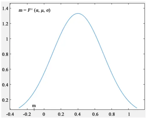
Given the portfolio wealth process by (2.10), it is clear that minimum portfolio wealth by high confidence level is reached when (2.11) obtains the lowest value by the same confidence level. In order to measure it, we need to know the prob-ability distribution function of portfolio returns. Once we have estimated the probability distribution function F for portfolio returns, we can extract the quantile _F−1

( )

_α _{, where alpha is a significance level, usually taken to be 1% or}

5%. The key improvement brought by the First Passage Time is that, if the esti-mated portfolio return probability density function does not turn out to be symmetric while the volatility is significantly large, then the portfolios’ expected bounded FPTs will often differ a lot. Graphically, if we denote MRL as

( )

1

m F₌ − α _{, on a normal distribution density function, it looks as follows}

[image:6.595.248.499.489.692.2]

(Figure 1).

(7)

From now on we will use m as the lowest level for the returns process (2.11) to reach in order to obtain the lowest portfolio wealth.

4. Expectation of Bounded First Passage Time.

Next step is to define the new dimension—expectation of bounded first passage time.

For a Brownian motion with drift

t t

X =µt W+ ₍_4.1)

if we denote the minimum value of this process till time t as:

inf

x

t s t s

M = ≤ X (4.2)

and let τ_y =min

{

t≥0;X_t ≤y

}

_{be the first passage time to the level y, then it is}

shown from [8] that the probability distribution function for

τ

y is given by:

(

x

)

(

)

_e2 y

t y y t y t

P M y P t N N

t t

µ

τ

 −   + 

≤ = ≤ = _ _+ _ _

    (4.3)

where N x

( )

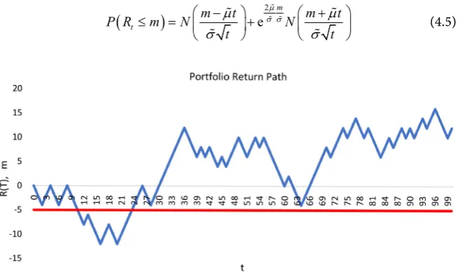
is the cumulative standard normal probability distribution func-tion.

We are looking for the first passage time for the returns process given by (2.11) towards the level m (which we called MRL). m is usually a negative quan-tity (Figure 2).

We know that R

( )

0 =0. In order for (2.11) to reach the m level, the follow-ing equation must be satisfied:

_t

m µ_{t B}

σ =σ + (4.4)

So, the first passage time τm=min

{

t≥0;Rt ≤m

}

has the probability

distri-bution function:

(

t

)

m t e2 m m t

P R m N N

t t

µ σ σ

µ µ

σ σ

− +

   

≤ = _ _+ _ _

   

  

 

[image:7.595.212.541.480.676.2]

  (4.5)

Figure 2. Blue graph is one possible path of the Brownian motion (2.11), red line is the m

level to which it can drop. MRL: m= −5%_{, Return process:}Rt=0.35 0.25t+ Bt,

(8)

If we have a Brownian motion with drift and diffusion given by:

dXt=µdt+σdWt (4.6)

and τ=min

(

t≥0;X_t ≤ y

)

_{, then it is shown in}_[8]_{that the probability density}

function of

τ

y is given by:

( )

2 0 2

0 2

2 3e

2π y

t y X t y X

f t

t

µ σ

τ

_σ

− + −

−

= (4.7)

Correspondingly by [9]

(

y

)

₀T _y

( )

d 1

(

y

)

E

τ

∧T =

∫

tf t t Tτ +  −P

τ

≤T  (4.8)

Converting (4.7) into the terms of R yields:

( )

( ( ))

2

0 2 2 3

0 e 2π m

t m R t m R

f t

t

µ σ

τ _σ

− + −

− =

 

 (4.9)

Thus

(

m

)

₀T _m

( )

d 1

(

m

)

E

τ

∧T =

∫

tf t t Tτ +  −P

τ

≤T  (4.10)

The reason we switch to the bounded first passage time is that since

( )

0 0

R = >m_{, from (2.11) it can be shown that for}µ>0,E

( )

τ_m = ∞. We al-ways consider portfolio return process which has a positive drift, because we examine only long portfolios in this paper.

5. Mean-MRL-FPT Framework

After having defined the portfolio wealth process, and MRL and expectation of the bounded first passage time, we can construct the model of portfolio optimi-zation. The goal is to find the maximum MRL and bounded First Passage Time for a given expected return for the investment end time T E R:

[ ]

_T =µT.

So, there are three dimensions giving the efficient set of portfolios.

(

)

[ ]

m T

E T

E R m

τ ∧

Varying the weights q q1, , ,2  qn allocated in the assets gives us the set of

different portfolios from which selecting the best combination of the above quantities yields the efficient surface (Figure 3).

On this surface, all risky portfolios are optimal in Mean-MRL-FPT sense since it is impossible to find a better combination of given quantities for each.

As an important note, the model is particularly useful when the individual as-sets within a portfolio have large variance causing the portfolio variance to be large as well. This makes the portfolio returns likely to hit the minimum level before the investment horizon. So, in this case E

(

τm∧T

)

<T and it makes

(9)

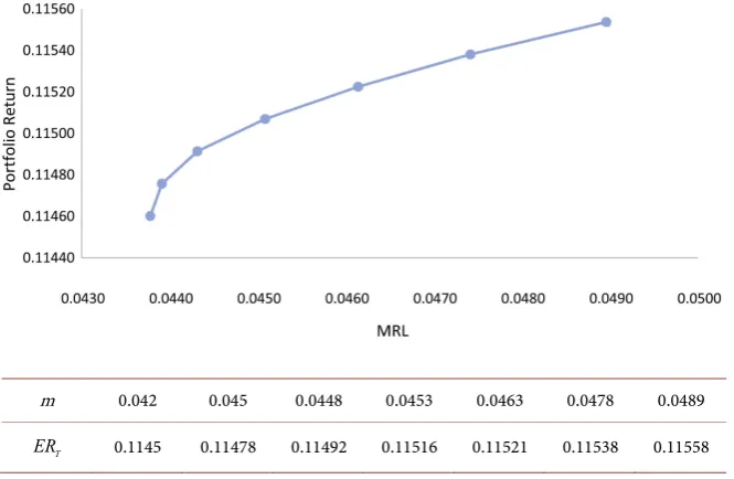
first passage time frequently coincides to the investment horizon-T. In this case,

(

m

)

[image:9.595.211.536.175.423.2]

E τ ∧T =T for any set of weights allocated to different assets and the first passage time can be dropped altogether and the decision is to be made solely on two dimensions—Mean and Minimum Return Level. In such a situation, we would obtain the two-dimensional curve that looks much like the efficient fron-tier (Figure 4).

Figure 3. Surface of portfolios obtained by different weights allocated to the assets in-cluded.

m 0.042 0.045 0.0448 0.0453 0.0463 0.0478 0.0489

T

ER 0.1145 0.11478 0.11492 0.11516 0.11521 0.11538 0.11558

Figure 4. Efficient frontier constructed by E R

( )

T and m F= −1

( )

α by different

[image:9.595.209.542.476.693.2]

(10)

6. Conclusions

The paper examined the portfolio selection process by introducing the frame-work involving three dimensions. The basic idea was to extend the two-dimensional framework by an additional one—the expected bounded first passage time. The usefulness of the approach is evident once the individual assets within a portfolio have large volatilities causing the returns to hit the minimum level before the investment horizon. The paper only concerned itself with optimizing risky port-folios. There can be numerous continuations to the problem. If an investor de-cides to allocate part of the investment amount into some risk-free assets, then the optimal weights must be modified according to some criteria. In two-dimensional Mean-Variance model, maximization of Sharpe ratio and building a Capital Allocation Line (CAL) is one possible development. Similarly, one may think of capital allocation plane as an analogue to CAL in 3D. However, this paper is restricted to risky portfolio optimization.

On a final note, as far as applicability of the model is concerned, it is obviously impossible to continuously rebalance the portfolio in order to maintain the con-stant weights. However, one can adopt some discretization methodology to find the optimal interval for making trades and taking transaction costs into account at the same time.

Conflicts of Interest

The author declares no conflicts of interest regarding the publication of this paper.

References

[1] Bookstaber, R. (1997) Global Risk Management: Are We Missing the Point? Journal of Portfolio Management, 23, 102-107.https://doi.org/10.3905/jpm.1997.102 [2] Boudoukh, J., Richardson, M., Stanton, R. and Whitelaw, R. (2004) MaxVar:

Long-Horizon Value-at-Risk in a Mark-to-Market Environment. Journal of Invest-ment ManageInvest-ment, 2, 14-19.https://doi.org/10.2139/ssrn.520805

[3] Artzner, P., Delbaen, F.., Eber, J.-M. and Heath, D. (1999) Coherent Measures of Risk. Mathematical Finance, 9, 203-228.https://doi.org/10.1111/1467-9965.00068 [4] Rockafellar, R.T. and Uryasev, S. (2000) Optimization of Conditional Value at Risk.

Journal of Risk, 2, 21-41.

[5] Chen, L., Peng, J., Zhang, B. and Rosyida, I. (2017) Diversified Models for Portfolio Selection Based on Uncertain Semi Variance. International Journal of Systems Science, 48, 637-648. https://doi.org/10.1080/00207721.2016.1206985

[6] Qin, Z.F., Kar, S. and Zheng, H.T. (2014) Uncertain Portfolio Adjusting Modelusing Semi Absolute Deviation. Soft Computing, 20, 717-725.

https://doi.org/10.1007/s00500-014-1535-y

[7] Dana, J. (2007) Financial Markets in Continuous Times. Springer-Verlag, Berlin, Heidelberg, New York.

[8] Shreve, S. (2008) Stochastic Calculus for Finance II. Springer Science & Business Media, New York.