A novel 2D image compression algorithm based on two levels DWT and DCT transforms with enhanced minimize matrix size algorithm for high resolution structured light 3D surface reconstruction

(1)

A novel 2D image compression algorithm based on two

levels DWT and DCT transforms with enhanced

minimize-matrix-size algorithm for high resolution structured light

3D surface reconstruction

SIDDEQ, M and RODRIGUES, Marcos

<http://orcid.org/0000-0002-6083-1303>

Available from Sheffield Hallam University Research Archive (SHURA) at:

http://shura.shu.ac.uk/10049/

This document is the author deposited version. You are advised to consult the

publisher's version if you wish to cite from it.

Published version

SIDDEQ, M and RODRIGUES, Marcos (2015). A novel 2D image compression

algorithm based on two levels DWT and DCT transforms with enhanced

minimize-matrix-size algorithm for high resolution structured light 3D surface reconstruction.

3D Research, 6 (3), p. 26.

Copyright and re-use policy

See

http://shura.shu.ac.uk/information.html

(2)

1

A Novel 2D Image Compression Algorithm based on two levels DWT and DCT

Transforms with Enhanced Minimize-Matrix-Size Algorithm for High Resolution

Structured Light 3D Surface Reconstruction

M. M. Siddeq and M. A. Rodrigues

GMPR-Geometric Modelling and Pattern Recognition Research Group, Shefﬁeld Hallam University, Shefﬁeld, UK

[email protected], [email protected]

Abstract

Image compression techniques are widely used in 2D and 3D image and video sequences. There are many types of compression techniques and among the most popular are JPEG and JPEG2000. In this research, we introduce a new compression method based on applying a two level Discrete Wavelet Transform (DWT) and a two level Discrete Cosine Transform (DCT) in connection with novel compression steps for high-resolution images. The proposed image compression algorithm consists of 4 steps: 1) Transform an image by a two level DWT followed by a DCT to produce two matrices: DC- and AC-Matrix, or low and high frequency matrix respectively; 2) apply a second level DCT to the DC-Matrix to generate two arrays, namely nonzero-array and zero-array; 3) apply the Minimize-Matrix-Size (MMS) algorithm to the AC-Matrix and to the other high-frequencies generated by the second level DWT; 4) apply arithmetic coding to the output of previous steps. A novel Fast-Match-Search (FMS) decompression algorithm is used to reconstruct all high-frequency matrices. The FMS-algorithm computes all compressed data probabilities by using a table of data, and then using a binary search algorithm for finding decompressed data inside the table. Thereafter, all decoded DC-values with the decoded AC-coefficients are combined into one matrix followed by inverse two level DCT with two level DWT. The technique is tested by compression and reconstruction of 3D surface patches. Additionally, this technique is compared with JPEG and JPEG2000 algorithm through 2D and 3D RMSE following reconstruction. The results demonstrate that the proposed compression method has better visual properties than JPEG and JPEG2000 and is able to more accurately reconstruct surface patches in 3D.

Keywords: DWT, DCT, Minimize-Matrix-Size Algorithm, FMS Algorithm, 3D reconstruction

1.

Introduction

Compression methods are being rapidly developed for large data files such as images, where data compression in multimedia applications has lately become more important. While it is true that the price of storage has steadily decreased, the amount of generated image and video data has increased exponentially. It is more evident on large data repositories such as YouTube and cloud storage offered by a number of suppliers. With the increasing growth of network traffic and storage requirements, more efficient methods are needed for compressing image and video data, while retaining high quality with significant reduction in storage requirements. The discrete cosine transform

(DCT) has been extensively used (Al-Haj, 2007; Taizo 2013) in image compression. The image is divided into

segments and each segment is then subject of the transform, creating a series of frequency components that correspond with detail levels of the image. Several forms of coding are applied in order to store only coefficients

that are found as significant. Such a way is used in the popular JPEG file format, and most video compression

methods and multi-media applications are generally based on it (Christopulos, 2000; Richardson, 2002).

A step beyond JPEG is JPEG2000 that is based on the discrete wavelet transform (DWT) which is one of the mathematical tools for hierarchically decomposing functions. Image compression using Wavelet Transforms is a powerful method that is preferred by scientists to get the compressed images at higher compression ratios with

higher PSNR values (Sadashivappa, 2002; Sayood, 2000). Its superiority in achieving high compression ratio, error

resilience, and other features led to JPEG2000 to be published as an ISO standard. As referred to the JPEG abbreviation, which stands for Joint Photographic Expert Group, JPEG2000 codec is more efficient than its

predecessor JPEG and overcomes its drawbacks (Esakkirajan, 2008). It also offers higher flexibility compared to

(3)

from its utilization of DWT for encoding image data. DWT exhibits high effectiveness in image compression due to its support to multi-resolution representation in both spatial and frequency domains. In addition, DWT supports

progressive image transmission and region of interest coding (Gonzalez, 2001; Acharya, 2005).

Furthermore, a requirement is introduced concerning the compression of 3D data. We demonstrated that while geometry and connectivity of a 3D mesh can be tackled by a number of techniques such as high degree polynomial

interpolation (Rodrigues, 2010) or partial differential equations (Rodrigues, 2013a; Rodrigues, 2013b), the issue

of efficient compression of 2D images both for 3D reconstruction and texture mapping for structured light 3D applications has not been addressed. Moreover, in many applications, it is necessary to transmit 3D models over the Internet to share CAD/CAM models with e-commerce customers, to update content for entertainment applications, or to support collaborative design, analysis, and display of engineering, medical, and scientific datasets. Bandwidth imposes hard limits on the amount of data transmission and, together with storage costs, limit the complexity of the 3D models that can be transmitted over the Internet and other networked environments. Using structured light techniques, it is envisaged that surface patches can be compressed as a 2D image together with 3D calibration parameters, transmitted over a network and remotely reconstructed (geometry, connectivity and texture map) at the

receiving end with the same resolution as the original data (Rodrigues, 2013c;Siddeq, 2014a).

Siddeq and Rodrigues in 2014 (Siddeq, 2014a) proposed a 2D image compression technique used in 3D

applications based on DWT and DCT. The DWT was linked with DCT to produce a series of high-frequency matrices, the same transformation applied again on the low-frequency matrix to produce another series of high-frequency data array. Finally data were coded by the Minimize-Matrix-Size Algorithm (MMS) and, at decompression stage, decoded by the Limited-Sequential Search Algorithm (LSS). The advantages of that proposed method were high-resolution image at high compression ratios up to 98%. However, the complexity of the algorithm meant long execution times, sometimes of the order of minutes for large 2D images.

In this paper we propose a new method for image compression based on two separate transformations: a two level DWT followed by a two level DCT applied to the low-frequency data leading to an increased number of high-frequency matrices, which are then shrunk using the Enhanced Minimize-Matrix-Size algorithm. This research demonstrates that the proposed algorithm achieves efficient image compression with ratios up to 99.5% and superior accurate 3D reconstruction compared with standard JPEG and JPEG2000.

The Proposed 2D Image Compression Algorithm

This section presents a novel lossy compression algorithm implemented via DWT and DCT. The algorithm starts

with a two level DWT. While all high frequencies (HL1, LH1, HH1) of the first level are discarded, all sub-bands of

the second level are further encoded. We then apply DCT to the low-frequency sub-band (LL2) of the second level;

the main reason for using DCT is to split into another low frequency and high-frequency matrices (DC- and

AC-Matrix1). The Enhanced Minimize-Matrix-Size (EMMS) algorithm is then applied to compress AC-Matrix1 and high

frequency matrices (HL2, LH2, HH2). The DC-Matrix1 is subject to a second DCT whose AC-Matrix2 is quantized

(4)

3

Fig. 1 Layout proposed two levels DWT-DCT Compression Technique

2.1

Two Level Discrete Wavelet Transform (DWT)

The implementation of the wavelet compression scheme is very similar to that of sub-band coding scheme: the

signal is decomposed using filter banks (Matthew 2010; Chen 2013). The output of the filter banks is

down-sampled, quantized, and encoded. The decoder decodes the coded representation, up-samples and recomposes the signal. Wavelet transform divides the information of an image into an approximation (i.e. LL) and detail sub-band. The approximation sub-band shows the general trend of pixel values and the other three detail sub-bands show the vertical, horizontal and diagonal details in the images. If these details are very small then they can be set to zero

without significantly changing the image details (Siddeq 2012b), for this reason the high frequency sub-bands are

compressed into fewer bytes. DWT uses filters for decomposing an image; these filters assist to increase the number of zeros in high frequency sub-bands. One common filter used in decomposition and composition is called Daubechies Filter. This filter stores much information about the original image in the "LL" sub-band, while other high-frequency domains contain less significant details, and this is one important property of the Daubechies filter for achieving a high compression ratio. A two-dimensional DWT is implemented on an image twice, first applied on

each row, and then applied on each column. (Sayood 2000; Richardson 2002):

In the proposed research the high frequency sub-bands at first level are set to zero (i.e. discard HL, LH and HH). These sub-bands do not affect image details. Additionally, only a small number of non-zero values are present in these sub-bands. In contrast, high-frequency sub-bands in the second level (HL2, LH2 and HH2) cannot be discarded, as this would significantly affect the image. For this reason, high-frequencies values in this region are quantized. The quantization process in this research depends on the maximum value in each sub-band, as shown by

the following equation (Siddeq, 2014b):

!!=_!!!

!! (1)

!!!=max !! ×!"#$% 2

Where, “H2” represents each high-frequency sub-band at second level in DWT (i.e. HL2, LH2 and HH2). While

“H2m” represents maximum value in a sub-band, and the "Ratio" value is used as a control for amount of maximum

value, which is used to control image quality. For example, if the maximum value in a sub-band is 60 and Ratio=0.1,

(5)

Each sub-band has different priority for keeping image details. The higher priorities are: LH2, HL2 and then HH2.

Most of information about image details is in HL2 and LH2. If most of nonzero data in these sub-bands are retained,

the image quality will be high even if some information is lost in HH2. For this reason the Ratio value for HL2,

LH2and HH2is defined in the range ={0.1 … 0.5}.

2.2

Two Level Discrete Cosine Transform (DCT)

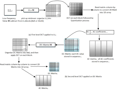
In this section we describe the two level DCT applied to low-frequency sub-band “LL2” (see Fig. 1). A quantization

is first applied to LL2 as follows. All values in LL2 are subtracted by the minimum of LL2and then divided by 2 (i.e.

a constant even number). Thereafter, a two-dimensional DCT is applied to produce de-correlated coefficients. Each variable size block (e.g. 8x8) in the frequency-domain consists of: the DC-value at the first location, while all the

other coefficients are called AC coefficients. The main reason for using DCT to split the final sub-band (LL2) into

two different matrices is to produce a low-frequency matrix (DC-matrix) and a high-frequency matrix (AC-Matrix). The following two steps are used in the two levels DCT implementation:

A- Organize LL2 into 8x8 non-overlapping blocks (other sizes can also be used such as 16x16) then apply

DCT to each block followed by quantization. The following equations represent the DCT and its inverse (Ahmed 1974; Sayood, 2000; Taizo 2013):

The quantization table is a matrix of the same block size that can be represents as follows:

! !,! =!"#$%+ !+! (3)

! !,! =! !,! ∗!"#$% (4)

Where: i, j=1,2,…Block , Scale=1,2,3,… Block

After applying the two-dimensional DCT on each 8x8 or 16x16block, each block is quantized by the “Q”

using dot-division-matrix, which truncates the results. This process removes insignificant coefficients and

increases the number of zeros in the each block. However, in the above Eq. (4), the factor "Scale" is used to

increase/decrease the values of "Q". Thus, image details are reduced in case of Scale>1. There is no limited

range for this factor, because this depends on the DCT coefficients.

B- Convert each block to 1D array, and then transfer the first value to a new matrix called DC-Matrix. While

the rest of data AC coefficients are saved into a new matrix called AC-Matrix. Similarity, the DC-Matrix is transformed again by DCT into another two different matrices: DCT-Matrix2 and AC-Matrix2. Fig. 2

(6)

5

Fig. 2 (a) and (b) two level DCT applied to LL2

The resulting DC-Matrix2 size is very small and can be represented in a few bytes. On the other hand, the

AC-Matrix2 contains lots of zeros with only a few nonzero data. All zero scan be erased and just nonzero data are

[image:6.612.101.506.72.389.2]

retained. This process involves separating zeros from nonzero data, as shown in Figure-3.The zero-array can be computed easily by calculating the number of zeros between two nonzero data. For example, assume the following AC-Matrix=[0.5, 0, 0, 0, 7.3, 0, 0, 0, 0, 0, -7], the zero-array will be [0,3,0,5,0] where the zeros in red refer to nonzero data existing at these positions in the original AC-Matrix and the numbers in black refer to the number of zeros between two consecutive non-zero data. In order to increase the compression ratio, the number “5” in the zero-array can be broken up into “3” and “2”zeros to increase the probability (i.e. re-occurrence) of redundant data. Thus, the new equivalent zero-array would become [0,3,0,3,2,0].

(7)

After this procedure, the nonzero-array contains positive and negative data (e.g. nonzero-array =[0.5,7.3,-7]), and each data size probably reaches to 32-bits and these data can be compressed by a coding method. In that case the index size (i.e. the header compressed file) is almost 50% of compressed data size. The index data are used in the decompression stage, therefore, the index data could be broken up into parts for more efficient compression. Each 32-bit data are partitioned into small parts (4-bit), and this process increases the probability of redundant data. Finally these streams of data are subject to arithmetic coding.

2.3

The Minimize-Matrix-Size Algorithm

In this section we introduce a new algorithm to squeeze high-frequency sub-bands into an array, then minimizing that array by using the Minimize-Matrix-Size algorithm, and then compressing the newly minimised array by arithmetic coding. Fig. 4 illustrates the steps in this novel high-frequency compression technique.

Fig. 4 Layout of the Minimize-Matrix-Size Algorithm

Each high-frequency sub-band contains lots of zeros with a few nonzero data. We propose a technique to eliminate block of zeros, and store blocks of nonzero data in an array. This technique is useful for squeezing all

high-frequency sub-bands, this process is labelled Eliminate Zeros and Store Nonzero data (EZSN) in Figure 4, applied to

each high frequency independently. The EZSN algorithm starts to partition the high-frequency sub-bands into non-overlapped blocks [K x K], and then search for nonzero blocks (i.e. search for at least one nonzero inside a block). If

a block contains any nonzero data, this block will be stored in the array called Reduced-Array, with the position of

that block. Otherwise, the block will be ignored, and the algorithm continues to search for other nonzero blocks. The EZSN algorithm is illustrated in List-1 below.

List-1:EZSN Algorithm

K=8; %% block size = [KxK] I=1; LOC=1

while (I< column size for high-frequency sub-band) J=1;

while (J< row size for high-frequency sub-band)

Block[1..K*K]= Read_Block_from_Matrix(I,J) ; %%8x8 block from high-frequency sub-band

if(Check_Block(Block) = = 'nonzero') %%check the "Block" content, has it a nonzero? POSITION [LOC] =I; POSITION [LOC+1] =J; %%Save original location for block contains

%%nonzero data in high-frequency sub-band LOC=LOC+2;

Forn=1: Block_Size* Block_Size

Reduced_Array[P]= Block[n]; %%save nonzero data in new array ++P;

(8)

7

Endwhile% inner loop

I=I+K; Endwhile

After each sub-band is squeezed into an array, thereafter, the Minimize-Matrix-Size Algorithm is applied to each reduced array independently. This method reduces the array size by 1/3, the calculation depends on key values and coefficients of the reduced array, and the result is stored in a new array called Coded-Array. The following equation represents the Minimize-Matrix-Size algorithm (Siddeq 2013; Siddeq 2014a; Siddeq 2014b):

CodedArray(P)=Key(1)*RA(L) + Key(2)*RA(L+1) + Key(3)*RA(L+2) (5)

Note that “RA” represents Reduced-Array (HL2, LH2, HH2 and AC-Matrix1)

L=1, 2, 3,… N-3, “N” is the size of Reduced-Array

P=1,2,3…N/3

The Key values in the above Eq.(5) are generated by a key generator algorithm. Initially compute the maximum value in reduced sub-band, and three keys are generated according to the following steps:

M=MAX_VALUE +(MAX_VALUE/2); %% maximum value selected and divided by “2”

Key[1]=0.1; %% First Key value <=1

Key[2]=[0.1× M ] ×Factor; %% Factor=1,2,3,…etc

Key[3]=[ KEY(1)× M+KEY(2)× M ] × Factor;

KEY=[Key[1], Key[2], Key[3]]; %% Final Key values for compression and decompression

Each reduced sub-band (See Fig. 4) has its own key value. This depends on the maximum value in each sub-band.

The idea for the key is similar to weights used in Perceptron Neural Network: P=AW1+BW2+CW3, where Wi are the

weight values generated randomly and “A”,“B” and “C” are data. The output of this summation is “P” and there is

only one possible combination for the data values given Wi (more details in section 3). Using a key generator the

Minimize-Matrix-Size algorithm illustrated in List-2(Siddeq, 2013;Siddeq 2014a;Siddeq 2014b).

List -2 : Minimize-Matrix-Size Algorithm

Let Pos=1

MAX_Value=Find_Max_value(Reduced-Array); W=Key-Generator(0.1, MAX_Value, 2); I=1;

while (I< size of Reduced-Array) For K=0 to 2

Coded-Array[Pos]= Coded-Array [Pos] + ( Reduced-Array[I+K] × W[K] ); Endfor

Pos++; I=I+3; Endwhile

Before applying the Minimize-Matrix-Size algorithm, our compression algorithm computes the probability of the

Reduced-Array (i.e. compute the probability for each HL2, LH2, HH2 and AC-Martix1). These probabilities are

called Limited-Data, which is used later in the decompression stage. The Limited-Data are stored as additional data

(9)

[image:9.612.114.492.337.589.2]

Fig. 5 Illustration of probability data (Limited-Data) for the Reduced-Array

The final step of the compression algorithm is arithmetic coding, which is one of the important methods used in data compression; its takes a stream of data and convert it to a single floating point value. These values lie in the range less than one and greater than zero that, when decoded, return the exact stream of data. The arithmetic coding needs to compute the probability of all data and assign a range for each data (low and high) in order to generate streams of

bits (Sayood, 2000).

2.

The Decompression Algorithm: Fast Matching Search Algorithm (FMS)

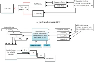
The proposed decompression algorithm is the inverse of compression and consists of three stages:

1) First level Inverse DCT to reconstruct the DC-Matrix1;

2) Apply the FMS-Algorithm to decode each sub-band independently (i.e. HL2, LH2, HH2, AC-Matrix2);

3) Apply the second level inverse DCT with two levels inverse DWT to reconstruct the 2D image.

Once the 2D image is reconstructed, we apply structured light 3D reconstruction algorithms to obtain an approximation of the original 3D surface, from which errors can be computed for the entire surface. Fig 6 shows the layout of the main steps in the proposed decompression algorithm.

(a) First level inverse DCT

(10)

9

(c) Two levels inverse DWT with two levels inverse DCT applied to decompress 2D image

Fig. 6(a), (b) and (c) represent layout of the proposed Decompression algorithm

The Fast Match Search Algorithm (FMS) has been designed to compute the original high frequency data. The

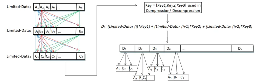
compressed data contains information about the compression keys and probability data (Limited-data) followed by streams of compressed high frequency data. Therefore, the FMS algorithm picks up each compressed high frequency data and reads information (key values and Limited-Data) from which the original high frequency data are recovered. The FMS-Algorithm is illustrated through the following steps A and B:

A) Initially, Limited-Data are copied (in memory) three times into separated arrays. This is because expanding

the compressed data with the three keys resembles an interconnected data, similar to a network as shown in Fig. 7.

B) Pick up a data item from“D”, the compressed array (i.e. Coded-HL2 or Coded-LH2 or Coded-HH2 or

Coded-AC-Matrix1) and search for the combination of (A,B,C) with respective keys that satisfy D. Return

[image:10.612.125.483.75.242.2]

the triplet decompressed values (A,B,C).

Fig. 7 First stage FMS-Algorithm for reconstructing high frequency data from Limited-Data. A, B and C are the uncompressed data which are determined by the unique combination of keys.

Since the three arrays of Limited-Data contain the same values, that is A1=B1=C1, A2=B2=C2, and so on the searching algorithm computes all possible combinations of A with Key1, B with Key2 and C with Key3 that yield a

result D. As a means of an example consider that Limited-Data1=[A1 A2 A3] , Limited-Data2=[B1 B2 B3] and

[image:10.612.99.509.484.617.2]

(11)

the equation is executed 27 times (33=27) testing all indices and keys. One of these combinations will match the data

in (D) (i.e. the original high frequency Coded-LH2 or Coded-HL2 or Coded-HH2 or Coded-AC-Matrix1) as described

in Fig. 6(b). The match indicates that the unique combination of A,B,C are the orgininal data we are after.

The searching algorithm used in our decompression method is called Binary Search Algorithm, the algorithm finds

the original data (A,B,C) for any input from array “D”. For binary search, the array should be arranged in ascending

order. In each step, the algorithm compares the input value with the middle of element of the array “D”. If the value

matches, then a matching element has been found and its position is returned (Knuth 1997). Otherwise, if the search

is less than the middle element of “D”, then the algorithm repeats its action on the sub-array to the left of the middle

element or, if the value is greater, on the sub-array to the right. There is no probability for “Not Matched”, because

the FMS-Algorithm computed all compression data possibilities previously.

After the Reduced-Arrays (LH2, LH2, HH2 and AC-Matrix1) are recovered, their full corresponding high frequency

matrices are re-build by placing nonzero-data in the exact locations according to EZSN algorithm (see List-1). Then

the sub-band LL2is reconstructed by combining the DC-Matrix1and AC-Matrix1 followed by the inverse DCT.

Finally, a two level inverse DWT is applied to recover the original 2D image (see Fig. 6(c)). Once the 2D image is decompressed, its 3D geometric surface is reconstructed such that error analysis can be performed in this dimension.

3.

Experimental Results

The results described below use MATLAB-R2013a for performing 2D image compression and decompression, and

3D surface reconstruction was performed with our own software developed within the GMPR group (Rodrigues et

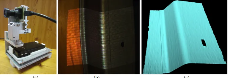
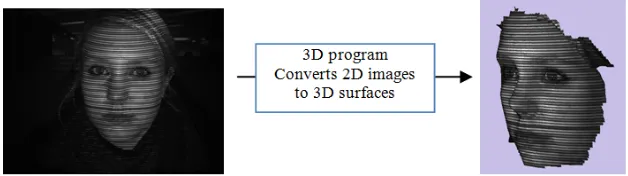
al. 2013a, 2013b, 2013c) running on an AMD quad-core microprocessor. The justification for introducing 3D reconstruction is that we can make use of a new set of metrics in terms of error measurements and perceived quality of the 3D visualization to assess the quality of the compression/decompression algorithms. The principle of operation of 3D surface scanning is to project patterns of light onto the target surface whose image is recorded by a camera. The shape of the captured pattern is combined with the spatial relationship between the light source and the camera, to determine the 3D position of the surface along the pattern. The main advantages of the method are speed and accuracy; a surface can be scanned from a single 2D image and processed into 3D surface in a few milliseconds (Rodrigues et al. 2013d). Fig. 8 shows a 2D image captured by the scanner then converted to a 3D surface by our 3D software.

[image:11.612.113.502.492.626.2]

(12)

11

The results in this research are divided into two parts: first, we apply the proposed image compression and decompression methods to 2D grey scale images of human faces. The original and decompressed images are used to generate 3D surface models from which direct comparisons are made in terms of perceived quality of the mesh and objective error measures such as RMSE. Second, we repeat all procedures for 2D compression and decompression, and 3D reconstruction but this time with colour images of objects other than faces. Additionally, the computed 2D and 3D RMSE are used directly for comparison with JPEG and JPEG2000 techniques.

4.1.Compression, Decompression and 3D Reconstruction from Grey Scale Images

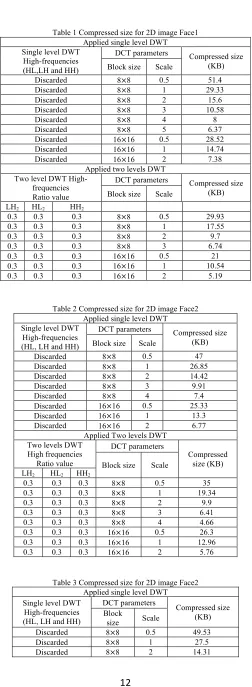
As described above the proposed image compression started with DWT. The level of DWT decomposition affects the image quality also the compression ratio, so we divided the results into two parts to show the effects of each independently: single level DWT and two level DWT. Fig. 9 shows the original 2D human faces tested by the proposed algorithm. Table 1, Table 2 and Table 3 show the compressed size by using our algorithm with a single level and two level DWT for Face1, Face2 and Face3 respectively.

(a) Original 2D Face1dimensions 1392 x 1040, Image size: 1.38 Mbytes, converted to 3D surface

(b) Original 2D Face2dimensions 1392 x 1040, Image size: 1.38 Mbytes, converted to 3D surface

(c) Original 2D Face3dimensions 1392 x 1040, Image size: 1.38 Mbytes, converted to 3D surface

[image:12.612.150.464.389.477.2]

(13)

[image:13.612.181.433.54.741.2]

Table 1 Compressed size for 2D image Face1 Applied single level DWT Single level DWT

High-frequencies (HL,LH and HH)

DCT parameters _{Compressed size} (KB) Block size Scale

Discarded 8×8 0.5 51.4

Discarded 8×8 1 29.33

Discarded 8×8 4 8

Discarded 16×16 0.5 28.52

Discarded 16×16 1 14.74

Applied two levels DWT Two level DWT

High-frequencies Ratio value

LH2 HL2 HH2

0.3 0.3 0.3 8×8 0.5 29.93

0.3 0.3 0.3 8×8 1 17.55

0.3 0.3 0.3 8×8 2 9.7

0.3 0.3 0.3 8×8 3 6.74

0.3 0.3 0.3 16×16 0.5 21

0.3 0.3 0.3 16×16 1 10.54

0.3 0.3 0.3 16×16 2 5.19

High-frequencies (HL, LH and HH)

Discarded 8×8 0.5 47

Discarded 16×16 0.5 25.33

Applied Two levels DWT Two levels DWT

High frequencies Ratio value

DCT parameters

Compressed size (KB) Block size Scale

LH2 HL2 HH2

0.3 0.3 0.3 8×8 0.5 35

0.3 0.3 0.3 8×8 1 19.34

0.3 0.3 0.3 8×8 2 9.9

0.3 0.3 0.3 8×8 3 6.41

0.3 0.3 0.3 8×8 4 4.66

0.3 0.3 0.3 16×16 0.5 26.3

0.3 0.3 0.3 16×16 1 12.96

[image:13.612.181.434.86.336.2]

0.3 0.3 0.3 16×16 2 5.76

DCT parameters

Compressed size (KB) Block

size Scale

Discarded 8×8 0.5 49.53

[image:13.612.192.422.352.681.2]

(14)

13

Discarded 16×16 0.5 26.83

Discarded 16×16 1 13.53

Applied Two levels DWT Two level DWT

High-frequencies Ratio value

DCT parameters

Compressed size (KB) Block

size Scale LH2 HL2 HH2

0.3 0.3 0.3 8×8 0.5 35.78

0.3 0.3 0.3 8×8 1 19.6

0.3 0.3 0.3 8×8 2 9.63

0.3 0.3 0.3 8×8 3 6.2

0.3 0.3 0.3 16×16 0.5 25.78

0.3 0.3 0.3 16×16 1 12.4

0.3 0.3 0.3 16×16 1.7 6.45

(a) This chart illustrates Table 1 for FACE1 image by using different scale values. The single level DWT and DCT (block size 16x16) is approximately close to the results obtained by two level DWT and DCT (block size 8x8).

(15)

(c) This chart illustrates Table 3 for FACE3 image by using different scale values. The single level DWT and DCT (block size 16x16) is approximately equivalent to the results obtained by two level DWT and DCT (block size 16x16).

Fig. 10 (a),(b) and (c) : illustrates Table 1, Table 2 and Table 3 as chart according to “Scale” and “Compressed Size”

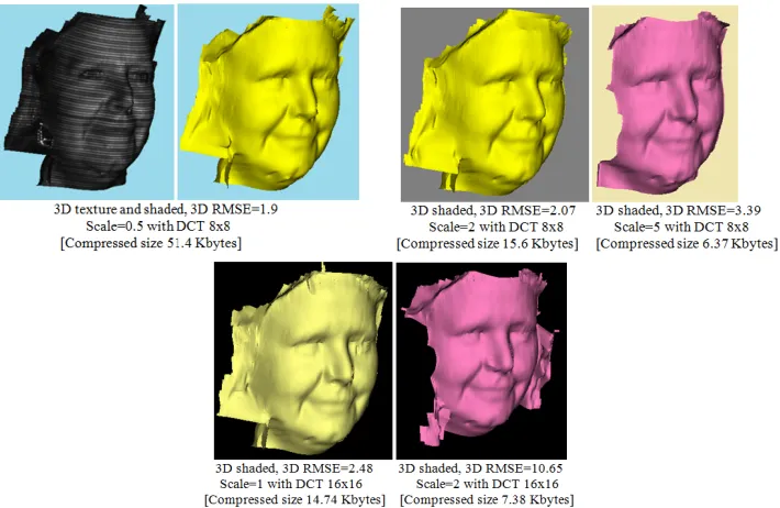
The proposed decompression algorithm (see Section 3) applied to the compressed image data recovers the 2D images which are then used by the 3D reconstruction algorithms to generate the respective 3D surface. Figures 11, 12 and 13 show high-quality, median-quality and low-quality compressed images for Face1, Face2 and Face3 respectively. Also, Tables 4, 5 and 6 show the time execution for the FMS-Algorithm.

(a) Decompressed 2D BMP images at Single level DWT converted to 3D surface; 3D surface with scale=0.5 represents high quality image comparable to the original image, and 3D surface with scale=2 represents median quality image approximately high quality image. Also 3D surface with scale=5 is low quality image some parts of surface failing to reconstruct. Additionally, using a block size

of 16×16 DCT further degrades the 3D surface.

[image:15.612.131.486.228.459.2]

(16)

15

[image:16.612.65.551.116.644.2]

Fig. 11 (a) and (b) decompressed 2D image Face1 by our proposed decompression method, and then converted to a 3D surface.

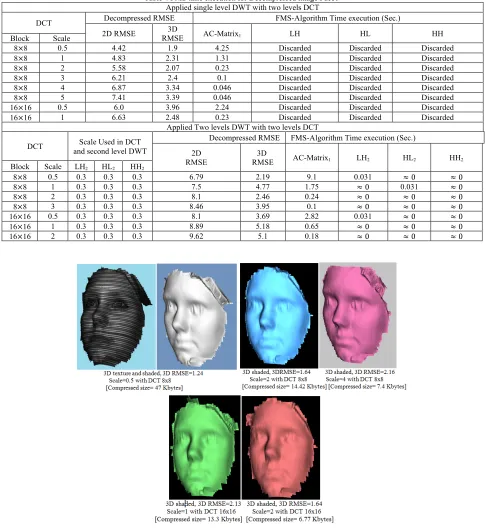
Table 4 FMS time execution for Decompressed image Face1 Applied single level DWT with two levels DCT

DCT Decompressed RMSE FMS-Algorithm Time execution (Sec.)

2D RMSE _RMSE3D AC-Matrix1 LH HL HH

Block Scale

8×8 0.5 4.42 1.9 4.25 Discarded Discarded Discarded

8×8 1 4.83 2.31 1.31 Discarded Discarded Discarded

16×16 0.5 6.0 3.96 2.24 Discarded Discarded Discarded

Applied Two levels DWT with two levels DCT

DCT _{and second level DWT}Scale Used in DCT Decompressed RMSE FMS-Algorithm Time execution (Sec.) 2D

RMSE

3D

RMSE AC-Matrix1 LH2 HL2 HH2

Block Scale LH2 HL2 HH2

8×8 0.5 0.3 0.3 0.3 6.79 2.19 9.1 0.031 ≈0 ≈0

8×8 1 0.3 0.3 0.3 7.5 4.77 1.75 ≈0 0.031 ≈0

8×8 2 0.3 0.3 0.3 8.1 2.46 0.24 ≈0 ≈0 ≈0

8×8 3 0.3 0.3 0.3 8.46 3.95 0.1 ≈0 ≈0 ≈0

16×16 0.5 0.3 0.3 0.3 8.1 3.69 2.82 0.031 ≈0 ≈0

16×16 1 0.3 0.3 0.3 8.89 5.18 0.65 ≈0 ≈0 ≈0

16×16 2 0.3 0.3 0.3 9.62 5.1 0.18 ≈0 ≈0 ≈0

(a) Decompressed 2D images at Single level DWT converted to 3D surface; 3D surface with scale=0.5 represents high quality image similar to the original image, and 3D surface with scale=2 represents a median quality image. Also 3D surface with scale=4 is low

(17)

(b) Decompressed 2D BMP images at two levels DWT converted to 3D surface; 3D surface with scale=2, 4 with DCT 8x8 represent low quality image surface with degradation. Similarly, a block size of 16x16 DCT used in our approach degrades the 3D surface.

Fig. 12 (a) and (b) Decompressed 2D image of Face2 image by our proposed decompression method, and then converted to 3D surface.

Table 5, FMS time execution for Decompressed image Face2 Applied single level DWT with two levels DCT

Block Scale

8x8 0.5 4.88 1.24 7 .06 Discarded Discarded Discarded

8x8 1 5.22 2.19 1.09 Discarded Discarded Discarded

16x16 0.5 5.57 1.7 3.4 Discarded Discarded Discarded

DCT Scale Used in DCT and second level DWT

Decompressed RMSE FMS-Algorithm Time execution (Sec.)

2D

RMSE RMSE 3D AC-Matrix1 LH2 HL2 HH2

8x8 0.5 0.3 0.3 0.3 5.16 1.33 13.15 0.046 0.046 0.031

8x8 1 0.3 0.3 0.3 5.76 2.07 2.1 0.031 ≈0 ≈0

8x8 2 0.3 0.3 0.3 7.04 2.04 0.35 0.062 ≈0 ≈0

8x8 3 0.3 0.3 0.3 7.91 1.39 0.109 ≈0 ≈0 ≈0

8x8 4 0.3 0.3 0.3 8.43 1.48 0.062 ≈0 ≈0 0.031

16x16 0.5 0.3 0.3 0.3 5.73 2.08 2.96 0.093 0.031 0.031

16x16 1 0.3 0.3 0.3 6.44 2.39 0.59 0.031 0.031 ≈0

16x16 2 0.3 0.3 0.3 7.85 3.16 0.124 0.015 ≈0 ≈0

[image:17.612.67.544.332.582.2]

(18)

17

(a) Decompressed 2D images at Single level DWT converted to 3D surface; 3D surface with scale=0.5 represent high quality image similar to the original image, and 3D surface with scale=2 represents median quality image, 3D surface with scale=3 and 4 are low quality image with slightly

degraded surface, while using 16x16 block size does not seem to degrade the 3D surface.

(b) Decompressed 2D images at two levels DWT converted to 3D surface; 3D surface with scale=3, 4 and DCT 8x8 represent low quality image degraded surface. However, the block size of 16x16 DCT used in our approach has a better quality 3D surface for higher compression ratios.

[image:18.612.115.499.73.339.2]

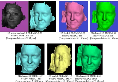
Fig. 13 (a) and (b): Decompressed 2D of Face3 image by our proposed decompression method, and then converted to a 3D surface.

Table 6, FMS time execution for Decompressed image Face3 Applied single level DWT with two levels DCT

Block Scale

8x8 0.5 4,29 1.26 5.91 Discarded Discarded Discarded

(19)

DCT

Scale Used in DCT and second level

DWT

Decompressed RMSE FMS-Algorithm Time execution (Sec.)

2D RMSE

3D

RMSE AC-Matrix1 LH2 HL2 HH2

8x8 0.5 0.3 0.3 0.3 4.81 1.13 12.00 0.078 0.046 ≈0

8x8 1 0.3 0.3 0.3 5.53 1.83 1.96 0.015 ≈0 ≈0

8x8 2 0.3 0.3 0.3 6.7 1.48 0.28 0.031 ≈0 ≈0

8x8 3 0.3 0.3 0.3 7.47 1.63 0.078 ≈0 0.031 ≈0

16x16 0.5 0.3 0.3 0.3 5.58 2.08 4.69 0.062 0.015 0.031

16x16 1 0.3 0.3 0.3 6.42 1.96 0.98 0.046 ≈0 ≈0

16x16 1.7 0.3 0.3 0.3 7.38 2.61 0.171 ≈0 ≈0 ≈0

It is shown through the pictures and tables above that the proposed compression algorithm is successfully applied to grey scale images. In particular, Tables 1, 2 and 3 show a compression of more than 99% of the original image size and the reconstructed 3D surfaces still preserve most of their original quality. Some images are compressed by DCT with block size of 16x16 are also shown capable of generating high quality 3D surface. Also there is not much difference between block sizes of 8x8 and 16x16 for high quality reconstruction images with “Scale=0.5”.

4.2.Compression, Decompression and 3D Reconstruction from Colour Images

Colour images contain red, green and blue layers. In JPEG and JPEG2000 colour layers are transformed to “YCbCr” layers before compression. This is because most of information about images is available in layer “Y” while other

layers “CrCb” contain less information (Gonzalez 2001; Takahiko 2008). The proposed image compression tested

with YCbCr layers, and then applied on true colour layers (Red, Green and Blue). Fig. 14 shows the original colour images tested by our approach.

(a) Original 2D “Wall”dimensions 1280 x 1024, Image size: 3.75 Mbytes, converted to 3D surface

(20)

19

(c) Original 2D “Corner”dimensions 1280 x 1024, Image size: 3.75 Mbytes, converted to 3D surface

Fig. 14 (a), (b) and (c) Original 2D images with 3D surface conversion

[image:20.612.149.465.75.164.2]

First the Wall, Room and Corner images as depicted in Fig. 14 were transformed to YCbCr before applying our proposed image compression– both using single level and two level DWT decomposition. Second, our approach was applied on the same colour images but this time using true colour layers. Table 7, 8 and 9 show the compressed size for the colour images by the proposed compression algorithm. Fig. 16, 17 and 18 show decompressed colour images (Wall, Room and Corner respectively) as 3D surface. Additionally, Tables 10, 11 and 12 illustrate the execution time for the FMS-Algorithm at single level DWT for the colour images. Similarly, Tables 13, 14 and 15 show the FMS-Algorithm time execution for the same colour images by using two levels DWT.

Table 7 Compressed sizes for 2D colour image Wall Applied single level DWT with two level DCT Single level DWT

High-frequencies (HL, LH and HH) For all colour layer

DCT parameters _{Compressed size} (KB) Block size _Y Scale _Cb _Cr

Ignored 8x8 0.5 1 1 26.3

Ignored 8x8 1 2 2 14.23

Ignored 8x8 2 4 4 7,53

Ignored 16x16 0.5 1 1 12.3

Ignored 16x16 1 2 2 6.55

Single level DWT High-Frequencies Block size Red Green Blue Compressed Size

Ignored 8x8 1 1 1 24.42

Ignored 8x8 3 3 3 8.47

Ignored 8x8 5 5 5 5.46

Ignored 16x16 1 1 1 11.47

Ignored 16x16 2 2 2 5.9

Ignored 16x16 2.5 2.5 2.5 4.85

Applied Two level DWT with two level DCT Two levels DWT High-frequencies

Ratio value for all colour layers

DCT parameters

Compressed size (KB)

Block size Scale

LH2 HL2 HH2 Y Cb Cr

0.3 0.3 0.3 8x8 0.5 1 1 28.1

0.3 0.3 0.3 8x8 1 2 2 11.8

0.3 0.3 0.3 16x16 0.5 1 1 21.8

0.3 0.3 0.3 16x16 1 2 2 8.29

Two levels DWT High-Frequencies Block size Red Green Blue Compressed Size

0.3 0.3 0.3 8x8 1 1 1 19.32

0.3 0.3 0.3 8x8 2 2 2 8.4

0.3 0.3 0.3 16x16 1 1 1 12.89

0.3 0.3 0.3 16x16 2 2 2 5

Table 8 Compressed size for 2D colour image Room Applied single level DWT with two level DCT Single level DWT

DCT parameters Compressed size (KB)

[image:20.612.132.484.352.660.2]

(21)

For all colour layer Y Cb Cr

Ignored 8x8 0.5 1 1 58.21

Ignored 8x8 1 2 2 34

Ignored 8x8 2 4 4 18.92

Ignored 16x16 0.5 1 1 29.86

Ignored 16x16 1 2 2 16.19

Ignored 16x16 2 4 4 8.07

Ignored 8x8 1 1 1 53.25

Ignored 8x8 3 3 3 17.66

Ignored 8x8 5 5 5 10.73

Ignored 8x8 9 9 9 6.28

Ignored 16x16 1 1 1 23.83

Ignored 16x16 3 3 3 7.91

Ignored 16x16 5 5 5 4.65

Ignored 16x16 7 7 7 3.38

DCT parameters

Block size Scale

LH2 HL2 HH2 Y Cb Cr

0.3 0.3 0.3 8x8 0.5 1 1 47.25

0.3 0.3 0.3 8x8 1 2 2 23.96

0.3 0.3 0.3 8x8 2 4 4 11.85

0.3 0.3 0.3 16x16 0.5 1 1 35.94

0.3 0.3 0.3 16x16 1 2 2 17.62

0.3 0.3 0.3 16x16 2 4 4 7.94

Two levels DWT High-Frequencies Block size Red Green Blue Compressed Size

0.3 0.3 0.3 8x8 1 1 1 49

0.3 0.3 0.3 8x8 3 3 3 10.42

0.3 0.3 0.3 8x8 5 5 5 5.12

0.3 0.3 0.3 16x16 1 1 1 36.34

0.3 0.3 0.3 16x16 3 3 3 6.61

[image:21.612.132.483.79.532.2]

0.3 0.3 0.3 16x16 5 5 5 2.93

Table 9 Compressed size for 2D colour image Corner Applied single level DWT with two level DCT Single level DWT

High-frequencies (HL, LH and HH) For all colour layer

DCT parameters Compressed size

Block size _Y _CbScale _Cr (KB)

Ignored 8x8 0.5 1 1 31.59

Ignored 8x8 1 2 2 15.85

Ignored 16x16 0.5 1 1 15.39

Ignored 16x16 0.8 6 6 7.8

Ignored 8x8 1 1 1 44.5

Ignored 8x8 2 2 2 22

Ignored 16x16 1 1 1 21.16

Ignored 16x16 2 2 2 10

DCT parameters

Block size Scale

LH2 HL2 HH2 Y Cb Cr

0.3 0.3 0.3 8x8 0.5 1 1 31.72

0.3 0.3 0.3 8x8 1 2 2 13.11

(22)

21

(a) Chart from Table 7 for Wall image by using different scale value in our approach, as shown in this figure the results obtained by our approach applied on RGB layers has better compression ratio than using YcbCr layers.

(b) Chart from Table 8 for Room image by using different scale value in our approach, as shown in this figure the results obtained by our approach applied on RGB layers has better compression ratio than using YcbCr layers.

(c) Chart from Table 9 for Corner image by using different scale value in our approach, as shown in this figure the results obtained by single level DWT with DCT (16x16) applied on YcbCr layers has better compression ratio than other options illustrated in this chart.

[image:22.612.121.492.72.224.2]

(23)

(a) Decompressed 2D images at single level DWT converted to 3D surface; decompressed 3D surface by using RGB layer has better quality than YCbCr layer.

(b) Decompressed 2D images at two levels DWT converted to 3D surface, also decompressed 3D surface using RGB layer has better quality than YCbCr layer at higher compression ratio.

[image:23.612.111.504.74.321.2]

(24)

23

(a) Decompressed 2D images at Single level DWT results converted to 3D surface; decompressed 3D surface by using RGB layer has better quality than YCbCr layer at higher compression ratio using both block sizes of 8x8 or 16x16 by DCT.

(b) Decompressed 2D images at two level DWT converted to 3D surface; decompressed 3D surface by using RGB layer has better quality than YCbCr layer at higher compression ratio using block sizes of 8x8, also by using block 16x16 the surface is still approximately non-degraded.

[image:24.612.132.480.71.286.2]

(25)

Fig. 18 Decompressed colour “Corner” image by our proposed decompression method, and then converted to 3D surface. The decompressed 3D surface at single level DWT using YCbCr has better quality at higher compression

ratio than using RGB layers, also at two level DWT degradation appears and some parts of the surface fail to reconstruct.

Table 10 Estimated execution time for FMS-Algorithm at single level DWT for Wall image

Compressed size

(KB) Block size

Time execution (Sec.)

Y Cb Cr

AC-Matrix1 AC-Matrix1 AC-Matrix1

26.3 8x8 1.77 0.093 0.187

14.23 8x8 0.202 0.031 0.078

7.53 8x8 0.062 ≈0 0.031

12.3 16x16 0.54 0.015 0.031

6.55 16x16 0.109 ≈0 0.031

Compressed size Block size _AC-MatrixRed Green Blue

1 AC-Matrix1 AC-Matrix1

24.42 8x8 0.12 1.27 0.12

8.47 8x8 ≈0 0.078 0.031

5.46 8x8 ≈0 0.046 ≈0

11.47 16x16 0.078 0.46 0.093

5.9 16x16 0.015 0.078 0.031

4.85 16x16 0.031 0.031 ≈0

[image:25.612.80.537.71.318.2]

Table 11 Estimated execution time for FMS-Algorithm at single level DWT for Room image Compressed size

(KB) Block size

Y Cb Cr

AC-Matrix AC-Matrix AC-Matrix

58.21 8x8 1.2 0.093 0.17

34 8x8 0.17 0.046 0.046

18.92 8x8 0.046 0.046 0.031

29.86 16x16 0.96 0.062 0.093

16.19 16x16 0.156 0.046 0.046

8.07 16x16 0.046 0.031 ≈0

Compressed size Block size _AC-MatrixRed _AC-MatrixGreen _AC-MatrixBlue

(26)

25

17.66 8x8 ≈0 0.124 0.015

10.73 8x8 ≈0 0.062 ≈0

6.28 8x8 ≈0 0.031 ≈0

23.83 16x16 0.046 0.68 0.078

7.91 16x16 ≈0 0.062 0.031

4.65 16x16 ≈0 0.046 ≈0

3.38 16x16 ≈0 0.031 ≈0

[image:26.612.166.447.72.142.2]

Table 12 Estimated execution time for FMS-Algorithm at single level DWT for Corner image Compressed size

(KB) Block size

Y Cb Cr

AC-Matrix AC-Matrix AC-Matrix

31.59 8x8 1.2 0.031 0.015

15.85 8x8 0.3 0.031 0.031

15.39 16x16 1.07 0.031 0.046

7.8 16x16 0.5 ≈0 ≈0

Compressed size Block size _AC-MatrixRed _AC-MatrixGreen _AC-MatrixBlue

44.5 8x8 0.34 0.48 0.34

22 8x8 0.06 0.09 0.09

21.16 16x16 0.46 0.48 0.37

10 16x16 0.1 0.14 0.1

Table 13 Estimated execution time for FMS-Algorithm at two level DWT for Wall image Compressed

size (KB)

Block size

Y Cb Cr

AC-Matrix1 HL2 LH2 HH2

AC-Matrix1 LH2 HL2 HH2

AC-Matrix1

HL2 LH2 HH2

28.1 8x8 3.1 0.062 0.062 0.031 0.062 0.03 ≈0 ≈0 0.24 0.031 ≈0 ≈0

11.8 8x8 0.6 0.015 ≈0 ≈0 0.046 0.031 ≈0 ≈0 0.046 0.031 ≈0 ≈0

21.8 16x16 1.5 0.031 0.031 ≈0 0.046 0.03 0.031 ≈0 0.093 0.031 ≈0 ≈0

8.29 16x16 0.026 0.015 ≈0 0.031 0.031 0.03 ≈0 ≈0 0.062 0.015 ≈0 ≈0

Compressed size

Block size

Red Green Blue

AC-Matrix1 HL2 LH2 HH2

AC-Matrix1

HL2 LH2 HH2

19.32 8x8 0.23 0 ≈0 ≈0 1.5 0.031 0.031 ≈0 0.26 ≈0 ≈0 ≈0

8.4 8x8 0.062 0.031 ≈0 ≈0 0.24 ≈0 ≈0 ≈0 0.078 ≈0 0.031 ≈0

12.89 16x16 0.21 0.078 ≈0 0.031 0.081 ≈0 ≈0 ≈0 0.17 ≈0 0 ≈0

5 16x16 0.062 ≈0 ≈0 ≈0 0.093 0.031 0.031 ≈0 0.062 ≈0 ≈0 ≈0

[image:26.612.164.450.215.344.2]

Table 14 Estimated execution time for FMS-Algorithm at two level DWT for Room image Compressed

size (KB)

Block size

Y Cb Cr

AC-Matrix1 HL2 LH2 HH2 AC-Matrix1 HL2 LH2 HH2 AC-Matrix1 HL2 LH2 LH2

47.25 8x8 0.15 0.046 ≈0 ≈0 0.1 0.031 0.031 ≈0 2.19 0.078 0.062 0.062

23.96 8x8 0.046 0.015 ≈0 ≈0 0.015 0.031 ≈0 ≈0 0.43 0.078 0.031 0.031

11.85 8x8 ≈0 ≈0 ≈0 ≈0 ≈0 0.031 ≈0 ≈0 0.078 0.015 ≈0 ≈0

35.94 16x16 0.124 0.031 ≈0 ≈0 0.078 0.015 0.031 ≈0 1.21 0.062 0.015 0.015

17.62 16x16 0.015 0.031 ≈0 ≈0 0.031 0.031 ≈0 ≈0 0.28 0.031 0.031 0.031

7.94 16x16 0.015 0.031 ≈0 ≈0 0.031 0.031 0.031 ≈0 0.093 0.031 ≈0 ≈0

Compressed size

Block size

Red Green Blue

AC-Matrix1 HL2 LH2 LH2 AC-Matrix1 HL2 LH2 HH2 AC-Matrix1 HL2 LH2 LH2

49 8x8 0.35 0.046 0.031 0.031 1.76 0.015 ≈0 ≈0 0.062 ≈0 ≈0 ≈0

10.42 8x8 0.046 ≈0 ≈0 ≈0 0.124 ≈0 ≈0 ≈0 ≈0 ≈0 ≈0 ≈0

5.12 8x8 0.031 ≈0 ≈0 ≈0 0.062 ≈0 ≈0 ≈0 ≈0 ≈0 ≈0 ≈0

36.34 16x16 0.17 0.046 0.062 0.062 1.27 0.031 ≈0 ≈0 0.015 0.031 ≈0 ≈0

6.61 16x16 ≈0 ≈0 ≈0 ≈0 0.1 ≈0 ≈0 ≈0 ≈0 ≈0 ≈0 ≈0

2.93 16x16 0.031 ≈0 ≈0 ≈0 0.062 ≈0 ≈0 ≈0 ≈0 0.031 ≈0 ≈0

[image:26.612.53.567.536.695.2]

(27)

Table 15 Estimated execution time for FMS-Algorithm at two level DWT for Corner image Compressed

size (KB)

Block size

Y Cb Cr

AC-Matrix1 LH2 HL2 HH2

31.72 8x8 4 0.016 0.031 ≈0 0.093 ≈0 0.015 ≈0 0.1 0.031 0.031 ≈0

13.11 8x8 0.85 ≈0 0.031 ≈0 0.031 ≈0 ≈0 ≈0 0.046 ≈0 0.031 ≈0

23.14 16x16 0.2.49 0.015 0.016 ≈0 0.062 0.031 ≈0 ≈0 0.1 0.031 0.031 ≈0

It can be seen from the above figures and tables that a single level DWT is applied successfully to the colour images using both YCbCr and RGB layers. Also the two level DWT gives good performance, however, two levels did not perform well on YCbCr layer at higher compression ratios. Both colour images Wall and Room contain structured patterns defined on the green layer; this renders RGB layers more appropriate to be used with the proposed approach. On the other hand, for the image Corner, the YCbCr layer proved more appropriate as the structured patterns are not defined over the green channel but spread across the layers.

4.3. Comparison with JPEG2000 and JPEG Compression Techniques

JPEG and JPEG2000 are both used widely in digital image and video compression, also for streaming data over the Internet. In this research we use these two methods for 3D image compression for comparison with our proposed approach. The JPEG technique is based on the 2D DCT applied to the partitioned image into 8x8 blocks, and then

each block encoded by RLE and Huffman encoding (Ahmed 1974; Liu, 2012). The JPEG2000 is based on the

multi-level DWT applied on the complete image and then each sub-band quantized and coded by Arithmetic

encoding (Acharya, 2005; Esakkirajan 2008). Most image compression applications depend on JPEG and

JPEG2000 and allow the user to specify a quality parameter to choose suitable compression ratios. If the image

quality is increased the compression ratio is decreased and vice versa (Sayood, 2000). The comparison of these

methods with our proposed one is based on similar compression ratios; we measured image quality by using Root-Mean-Square-Error (RMSE). The RMSE is a very popular quality measure, and can be calculated very easily

between decompressed and original images (Sayood, 2000; Gerald 2014).We also show visualizations of 3D

surfaces for decompressed 2D images by JPEG and JPEG2000 as a means of comparison.

Table 16 Comparison JPEG2000 and JPEG with our approach for Face1 image

Our Proposed algorithm JPEG2000 JPEG

Compressed Size (KB) 2D RMSE 3D RMSE 2D RMSE 3D RMSE 2D RMSE 3D RMSE

≈26.85 5.22 2.19 4.1 1.51 8.57 1.67

≈14.42 5.86 1.64 5.3 2.68 Not Applicable Not Applicable

Proposed algorithm JPEG2000 JPEG

Compressed

Size (KB) RMSE2D RMSE3D RMSE2D RMSE3D RMSE2D RMSE3D

≈29.33 4.83 2.31 3.48 3.31 12 2.73

(28)

27

[image:28.612.108.504.123.193.2]

Compressed

Size (KB) RMSE 2D RMSE 3D RMSE 2D RMSE 3D RMSE 2D RMSE 3D

≈27.5 4.7 1.32 3.83 1.25 7.64 1.78

Table 19 Comparison JPEG2000 and JPEG with our approach for Wall image

≈26.3 4.37 1.96 2.63 0.31 9.66 0.66

Table-20 comparison JPEG2000 and JPEG with our approach for Room image

≈17.66 6.36 0.12 7.59 0.23 20 113.59 (not matched)

≈3.38 9.22 2.21 13.59 94.67 (not matched) Not Applicable Not Applicable

≈2.93 11.26 0.42 15.06 Not Applicable Not Applicable Not Applicable

Table-21, comparison JPEG2000 and JPEG with our approach for Corner image

Compressed Size (KB)

2D RMSE

3D

RMSE 2D RMSE 3D RMSE 2DRMSE 3DRMSE

≈31.59 3.58 1.78 3.12 1.92 5.86 16.46

(29)

[image:29.612.113.495.73.210.2]

Fig. 19 Decompressed 2D Face1 image by using JPEG2000 and JPEG algorithm, JPEG algorithm can’t compress the 2D Face1 image under 29 KB.

[image:29.612.89.523.266.396.2]

Fig.20 Decompressed 2D Face2 image by using JPEG2000 and JPEG algorithm degradation appeared by JPEG on the surface at 26 KB.

Fig. 21 Decompressed 2D Face3 image by using JPEG2000 and JPEG algorithm, parts of images failed to reconstruct in 3D by JPEG2000 algorithm at 14 KB, degradation appears on the surface by JPEG2000 under 7 KB,

[image:29.612.95.512.471.604.2]

(30)

[image:30.612.113.503.74.277.2]

29

Fig. 22 Decompressed Wall image by using JPEG2000 and JPEG algorithm, degradation appears on surface by JPEG2000 fewer than 12 KB, also JPEG algorithm degrades the surface at compressed size 27 KB, JPEG fails to

compress under 27 KB.

[image:30.612.158.459.353.634.2]

(31)

[image:31.612.153.456.70.420.2]

Fig. 24 Decompressed Corner image by using JPEG2000 and JPEG algorithm, top-left surface decompressed successfully by JPEG2000, in top-right decompressed surface by JPEG2000 not matched with original surface (grey

surface). Under 15 KB, similarly, JPEG algorithm fails to compress successfully fewer than 31 KB.

5. Conclusion

This research has presented and demonstrated a novel method for image compression and compared the quality of compression through 3D reconstruction, 3D RMSE and the perceived quality of the 3D visualisation. The method is based on a two level DWT transform and two level DCT transform in connection with the proposed Minimize-Matrix-Size algorithm. The results showed that our approach introduced better image quality at higher compression ratios than JPEG and JPEG2000 being capable of accurate 3D reconstructing at higher compression ratios. On the other hand, it is more complex than JPEG2000 and JPEG. The most important aspects of the method and their role in providing high quality image with high compression ratios are discussed as follows:

1- In a two levels DCT, the first level separates the DC-values and AC-values into different matrices; the second level

DCT is then applied to the DC-values and this generates two new matrices. The size of the two new matrices are only a few bytes long (because they contain a large number of zeros), this process increases the compression ratio.

2- Since most of the high-frequency matrices contain a large number of zeros as above, in this research we used the

(32)

31

3- The Minimized-Matrix-Size algorithm is used to replace each three coefficients from the high-frequencies matrices

by a single floating-point value. This process converts each high-frequency matrix into a one-dimensional array, leading to increased compression ratios while keeping the quality of the high-frequency coefficients.

4- The FMS-Algorithm represents the core of our search algorithm for finding the exact original data from a

one-dimensional array (i.e. Reduced-Array) converting to a matrix, and depends on the organized key-values and Limited-Data. According to time execution tables, the FMS-Algorithm finds values in a few milliseconds, for some high-frequencies needs just few microseconds at higher compression ratios.

5- The key-values and Limited-Data are used in coding and decoding an image, without these information images

cannot be reconstructed.

6- Our proposed image compression algorithm was tested on true colour images (i.e. Red, Green and Blue), obtained

higher compression ratios and high image quality for images containing green structured patterns. Additionally, our approach has been tested on YCbCr layers with good quality at higher compression ratios.

7- Our approach gives better visual image quality compared to JPEG and JPEG2000. This is because our approach

removes most of the block artefacts caused by the 8x8 two-dimensional DCT. Also our approach uses a single level DWT or two level DWT rather than multi-level DWT as in JPEG2000; for this reason, blurring typical of JPEG2000 is removed in our approach. JPEG and JPEG2000 failed to reconstruct a surface in 3D when compressed to higher ratios while it is demonstrated that our approach can successfully reconstruct the surface and thus, is superior to both on this aspect.

However, there are a larger number of steps in the proposed compression and decompression algorithm than in JPEG and JPEG2000. Also the complexity of FMS-algorithm leads to increased execution time for decompression, because the FMS-Algorithm is based on a binary search method. Future work includes search optimization of the FMS algorithm, as per current implementation this is a constraining step for real-time applications such as video data streaming over the Internet.

References

[1] A. Al-Haj, (2007) Combined DWT-DCT Digital Image Watermarking, Science Publications, Journal of

Computer Science 3 (9): 740-746.

[2] C. Christopoulos, J. Askelof, and M. Larsson (2000) Efficient methods for encoding regions of interest in the

upcoming JPEG 2000 still image coding standard, IEEE Signal Processing Letters,vol.7,no.9.

[3] C. Matthew, Stamm and K. J. Ray Liu, (2010), WAVELET-BASED IMAGE COMPRESSION

ANTI-FORENSICS, Proceedings of 2010 IEEE 17th International Conference on Image Processing September 26-29,

2010, Hong Kong: 1737-1740

[4] G. SadashivappaandK.V.S.AnandaBabu, (2002) PERFORMANCE ANALYSIS OF IMAGE CODING USING

WAVELETS, IJCSNS International Journal of Computer Science and Network Security, VOL.8 No.10.

[5] Gerald Schaefer (2014), Soft computing-based colour quantization, EURASIP Journal on Image and Video

Processing, doi:10.1186/1687-5281-2014-8

[6] I.E. G. Richardson (2002) Video Codec Design, John Wiley &Sons.

[7] K. Sayood, (2000) Introduction to Data Compression, 2nd_{edition, Academic Press, Morgan Kaufman Publishers.}

[8] Kuo-Cheng Liu, (2012), Prediction error preprocessing for perceptual color image compression, EURASIP

Journal on Image and Video Processing 2012, doi:10.1186/1687-5281-2012-3

[9] Knuth, Donald (1997). Sorting and Searching: Section 6.2.1: Searching an Ordered Table, The Art of

Computer Programming 3 (3rd Ed.), Addison-Wesley. pp. 409–426. ISBN 0-201-89685-0

[10] M. M. Siddeq, (2012a), Using Two Levels DWT with Limited Sequential Search Algorithm for Image

Compression, Journal of Signal and Information Processing, DOI:10.4236/jsip.2012.31008 Published Online

February 2012 (http://www.SciRP.org/journal/jsip) : 51-62

[11] M. M. Siddeq, (2012b), Using Sequential Search Algorithm with Single level Discrete Wavelet Transform for

Image Compression (SSA-W), Journal of Advances in Information Technology. Academic Publisher Vol. 3,No.

4.

[12] M. Rodrigues, A. Robinson and A. Osman, (2010) Efficient 3D data compression through parameterization of

free-form surface patches, In: Signal Process and Multimedia Applications (SIGMAP), Proceedings of the 2010

(33)

[13] M. M. Siddeq, G. Al-Khafaji, (2013) Applied Minimize-Matrix-Size Algorithm on the Transformed images

by DCT and DWT used for image Compression, International Journal of Computer Applications, Vol.70, No. 15.

[14] M. M. Siddeq, Prof. M. Rodrigues, (2014a) A New 2D Image Compression Technique for 3D Surface

Reconstruction, 18th_{International Conference on Circuits, Systems, Communications and Computers, Santorin}

Island, Greece: 379-386

[15] M. M. Siddeq, M. A. Rodrigues(2014b) A Novel Image Compression Algorithm for high resolution 3D

Reconstruction, 3D Research. Springer Vol. 5 No.2.DOI 10.1007/s13319-014-0007-6

[16] M. Rodrigues, A. Osman and A. Robinson, (2013a) Partial differential equations for 3D data compression and

reconstruction, Journal Advances in Dynamical Systems and Applications.12(3), 2004, pp 371–378

[17] M. Rodrigues, M. Kormann, C.Schuhler and P. Tomek(2013b) Robot trajectory planning using OLP and

structured light 3D machine vision. Lecture notes in Computer Science Part II. LCNS, 8034 (8034).

Springer,Heidelberg, 244-253.

[18] M. Rodrigues, M. Kormann, C.Schuhler and P. Tomek (2013c). Structured light techniques for 3D surface

reconstruction in robotic tasks

.

In: KACPRZYK, J, (ed.) Advances in Intelligent Systems and

Computing.Heidelberg, Springer, 805-814.

[19] M. Rodrigues, M. Kormann, C.Schuhler and P. Tomek (2013d). An intelligent real time 3D vision system

for robotic welding tasks. In: Mechatronics and its applications. IEEE Xplore, 1-6.

[20] M. Rodrigues, WILLIE BRINK and A. Robinson, (2007) Issues in Fast 3D Reconstruction from Video

Sequences, Proceedings of the 7th WSEAS International Conference on Multimedia, Internet & Video

Technologies, Beijing, China, September 15-17.

[21] N. Ahmed, T. Natarajan and K. R. Rao, (1974) Discrete cosine transforms, IEEE Transactions Computer.,” vol.

C-23, pp. 90-93.

[22] P. Chen, Jia-Y. Chang (2013) An Adaptive Quantization Scheme for 2-D DWT Coefficients, International

Journal of Applied Science and Engineering Vol.11, No. 1.

[23] S. Esakkirajan, T. Veerakumar, V. SenthilMurugan, and P. Navaneethan, (2008) Image Compression Using

Multiwavelet and Multi-stage Vector Quantization, International Journal of Signal Processing Vol. 4, No.4,

WASET.

[24] R. C. Gonzalez, R. E. Woods (2001) Digital Image Processing, AddisonWesleypublishing company.

[25] T. Acharya and P. S. Tsai. (2005) JPEG2000 Standard for Image Compression: Concepts, Algorithms and VLSI

Architectures. New York: John Wiley & Sons.

[26] Taizo Suzuki and Masaaki Ikehara (2013), Integer fast lapped transforms based on direct-lifting of DCTs for

lossy-to-lossless image coding, EURASIP Journal on Image and Video Processing,

doi:10.1186/1687-5281-2013-65

[27] Takahiko Horiuchi and Shoji Tominaga, (2008) Color Image Coding by Colorization Approach, EURASIP

http://shura.shu.ac.uk/information.html

http://shura.shu.ac.uk