Abstract—An important facet of infrastructure project
development is to achieve a dynamic balance between benefits and cost throughout the project’s life cycle. However, in light of the uncertainty of a range of critical parameters governing this balance, it is rather challenging for project decision makers to adequately assess a project’s feasibility. A risk-based, cost-benefit analytical framework to explore the feasibility of a project is proposed to aid decision making and provide recommendations. Uncertainty modeling is employed through the use of the Hasofer-Lind method or advanced first-order second-moment analysis. The framework developed brings together concepts from engineering reliability analysis, life cycle costing, autoregression, and uses the risk metric of probability of loss. This paper presents the logic behind the approach and tests the framework using a synthetic residential property project formulated around the economic perspective of an investor. It studies the effects of variations in cost and benefits, with particular focus on the uncertainty of future benefits. It was found that as the variation in total benefit increases, the probability that the investment would make a loss increases. For this study’s scenario when the coefficient of variation of benefits (CVB)increased by 5%, the probability of loss (Pf) increased by almost 10%. Furthermore, when the expected benefit exceeds the expected cost, large uncertainty in benefits are seen as negative risk and would increase the chance of investment loss. An increase in CVB by 25% led to an increase of 15.8% in Pf. It was also found that low levels of benefit variation do not have a large effect on Pf for a given low cost level.
In contrast, when the expected cost exceeds expected benefits, large uncertainty in benefit is seen as positive risk and would decrease the chance of investment loss. An increase in CVB by 25% led to a decrease in Pf by 22.1%.
A study of investors’ preference to risk was also carried out and it was found that for all levels of risk preference, increasing the uncertainty of future benefit should encourage investors to decrease their exposure to cost uncertainty in order to maintain their acceptable risk level. In addition, a small increase in variation in benefit has a larger effect on risk averse investors.
Manuscript received June 30, 2013; revised July 29, 2013. This work was supported by the Australian Postgraduate Award, awarded by the University of Melbourne, and the Melbourne Sustainable Society Institute (MSSI) of the University of Melbourne.
J. Lai is with the Department of Infrastructure Engineering, The University of Melbourne, Parkville 3010, Victoria, Australia (phone: +613 8344 4955; e-mail: [email protected]).
L. Zhang is with the Department of Infrastructure Engineering, The University of Melbourne, Parkville 3010, Victoria, Australia (e-mail: [email protected]).
C.F. Duffield is with the Department of Infrastructure Engineering, The University of Melbourne, Parkville 3010, Victoria, Australia (e-mail: [email protected]).
L. Aye is with the Department of Infrastructure Engineering, The University of Melbourne, Parkville 3010, Victoria, Australia (e-mail: [email protected]).
Index Terms— AFOSM, life cycle analysis, property
development, reliability analysis, risk management.
I. INTRODUCTION
ncertainty surrounding infrastructure projects stems from both non-cognitive and cognitive sources [1], and it is impossible to eliminate uncertainty completely. As projects may be worth millions of dollars involving many interested investors, modeling such uncertainty is necessary to determine project feasibility. Reliability analysis evaluates the uncertainty of model outputs in relation to uncertainties within the model of the system [2]. It has traditionally been applied to structural engineering designs involving resistance and loading [1], [3] but has also been extended for application in other areas such as in reservoir systems and water allocation problems [2], design of composition channels involving runoff uncertainty [4], and dissolved oxygen concentrations in water quality applications [5]. In this framework, monetary benefits (B)
and costs (C) are taken as analogous to resistance and
loading respectively. The concept of implementing reliability methods to evaluate the uncertainty of cost and benefit in infrastructure project appraisals has been introduced in a study by Lai, Zhang, Duffield and Aye [6]. The formulation of the model included employing the order second-moment (FOSM) method or mean value first-order second-moment (MVFOSM) method in an application of a synthesized desalination plant in Victoria, Australia. The study summarized the risk profile of a project with the following risk metrics: Value at Risk, reliability index (β) and probability of loss (Pf). This paper extends the
framework with advanced first-order second-moment (AFOSM), also known as the Hasofer-Lind method. Studies have shown that AFOSM provides a better method of calculating risk compared to MVFOSM. MVFOSM was considered to be inferior as it does not account for the variables’ distributional information when known, and also provides less accurate solutions when the performance function is non-linear [1]. Furthermore, MVFOSM exhibits an invariance problem whereby the calculated β is different despite the safety margin being defined in a mathematically equivalent manner [1], [3]. AFOSM is an invariant reliability analysis method [2] and the solutions are independent of the expression of the performance function. Additionally, there is an added potential for it to be
Financial Risk Analysis for Engineering
Management: A Framework Development and
Testing
J. Lai, L. Zhang, C.F. Duffield, and L. Aye
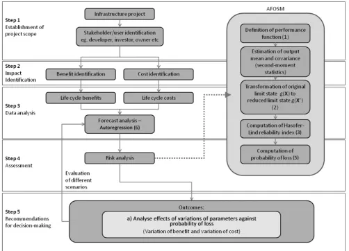
Fig. 1. Risk model framework
employed in the assessment of non-monetary variables as it deals with unit-less numbers in determining β. Monte Carlo simulation is another popular tool that allows estimation of the reliability of a system. However, the advantage of AFOSM over Monte Carlo simulation is its less restrictive computational demands, especially for complex models with multiple parameters [2], [5]. Fig. 1 shows the framework employed in this study and the objectives of this paper are to: a) apply reliability analysis using AFOSM to cost and benefit variables in an infrastructure project; and b) evaluate the effects of varying the extent of uncertainty on project design, focusing particularly on benefit uncertainty.
II. THEORETICALFRAMEWORKOFUNCERTAINTY MODELING
A. Reliability analysis
It is important for investors to balance cost and benefit in an infrastructure project, thus it is reasonable to assume that a project should be feasible where benefit or inflow of cash,
B, exceeds costs or outflow, C. Let the difference between B
and C be defined by random variables X1, X2, ..., Xn. The
probability of loss, Pf, for a system is defined as the
probability when C exceeds B, as shown in (1), where NPV = B – C = g X1, X2, ... , Xn is the performance function or
safety margin made up of multiple random variables Xn.
p P B P NPV 0 (1)
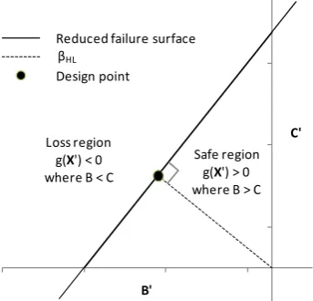
AFOSM identifies the point of design of the system at the most probable point of loss when the performance function is set to 0 (i.e. B = C), such that NPV = 0 provides the
failure surface or limit state. The failure surface is evaluated in a reduced system where variables are standardized to
X (2)
In the reduced system, the failure surface equation becomes 0 with random variables g(X , X , . . . , X , and B’ and C’ as reduced benefit and cost.
The mean and standard deviation are represented by µ and σ respectively of the random variables B and C. Fig. 2
illustrates the AFOSM concept with B’ and C’ intercepts
– , 0 and 0, respectively. The acceptable (or design) point is defined by the shortest distance between the failure surface and the point of origin in the reduced coordinate system. This represents the point of minimum reliability [4] or the most probable point of failure [1].The loss region occurs when g(X’) < 0. The nearer the failure
surface is to the origin in the reduced coordinate system, the larger the loss region will be.
The minimum distance in the reduced coordinate system is represented by the reliability index, βHL, in (3), where *
indicates that it is calculated at the design point ∗ .
∗ ∗
∑ ∗ ∗
∑ ∗
Fig. 2. Reduced coordinate system for benefit, B’, and cost, C’
α represents directional cosines along the reduced coordinate :
∝
∗
∑ ∗
(4)
Pf is the probability of a system failing its functions [5] and
is expressed in (5). It gives the region of PDF of the standardized normal variates between –∞ and –βHL, where
is the cumulative distribution function of the standard normal variates.
p Φ β 1 Φ β 5 In this study, random variables are assumed to be statistically normal and independent.
B. Forecasting
Forecasting future benefits and costs accurately is challenging. The framework employs autoregression to forecast costs and benefits by assuming independent variables are time-lagged versions of the dependent variables. This technique was used by Nagaraja, Brown and Zhao [7] in house price modeling as it was relatively straight forward to incorporate. As the building industry is likely to experience market shocks that would carry onto the next period, autoregression would be a useful tool to model this behavior. The general form of the model is shown in (6).
∑ (6)
where xt = value in the current year
a1, a2, ..., am = autoregression coefficients, estimated
from least-squares regression p = order of the model
x(t -1) = value in the previous year
Ɛt = output uncorrelated errors
The most significant order, p, is generated by applying a time-lag that produces a p-value of the highest order coefficient less than 0.05, which enables the rejection of the null hypothesis assuming the null hypothesis is true. That is, a 5% probability of a Type I error in rejecting the null hypothesis when it is true [8]. The coefficients a1, a2,..., am
indicate the weighting of previous years and define the strength of the relationship between current year and lagged periods. The general steps for determining the appropriate order of a model for this paper are briefly described: a) scope and time horizon of historical cost and benefit are identified; b) using different order of lag operators, the cost and benefit variables are regressed multiple times; c) the significance of the model order is compared at a 0.05
significance level; d) the order that is statistically significant is identified when the p-value of the highest order coefficient is smaller than the significance level, any higher order is redundant; and e) regressed values are compared with actual data to identify inconsistencies.
It is possible to use expert judgment to construct the ranges of coefficients if historical data are inadequate for prediction into future periods [9]. It is also possible to subjectively adjust the forecast to accommodate known changes that would take place, such as a change in government policy, however these assumptions would need to be clearly stated and justified.
III. RESULTS AND DISCUSSION
In this study, the theoretical framework is applied to a residential building investment. The building is a two-storey middle-class house, medium in size, and located in metropolitan Melbourne, Australia. The first floor is approximately 167 m2 and the second floor is 130 m2. For
modeling purposes, the house prices used for forecasting were sourced from Melbourne median prices dated from 1966 to 2012. These were extracted from The Real Estate Institute of Victoria [10]. Data for house price included inflation. Construction costs were derived from the Australian Construction Handbook by Rawlinsons from years 1983 to 2010. Household utility data were obtained from the Essential Services Commission. The standard tariffs for 2008 could have been significantly affected by the effect of drought conditions in Eastern Australia. This paper considers the financial implications from an investor’s point of view. For simplicity, only house price is considered as a univariate random variable. Distribution probabilities of parameters are inferred from Monte Carlo simulation in the absence of data. Social and environmental aspects, whilst important, were not considered within the scope of this paper.
The paper focuses on evaluating the effects of uncertainty of future cash inflows of the project, which are regarded as the benefits. These include rental income, land value at resale and house price at resale. The costs include land purchase price, construction cost, stamp duty, land tax, loan interests at 7%, and council rates. A discount rate of 5% has been used. As the variation of parameters is likely to change over time, all the results are evaluated at the asset being purchased in 2013, and held and sold in 15 years time. Deterministically when the asset is held for 15 years, the benefit is expected to exceed cost with expected mean of µB
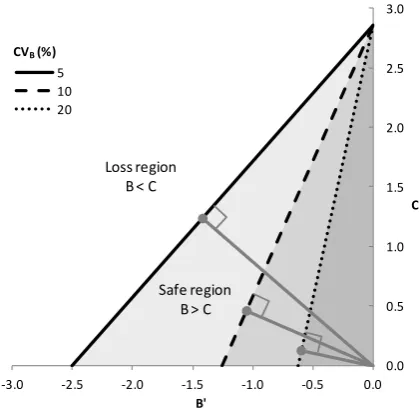
= $1,628,865 and µC = $1,428,567 respectively. Fig. 3a
shows the change in design point and loss region for different values of coefficient of variation of benefit, CVB,
in the Hasofer-Lind reduced space. The failure surface represents the boundary of the loss region, where investor cost is expected to exceed benefit. The loss region increases as CVB increases. Furthermore, the lines from the origin
connecting perpendicular to the failure surface represents βHL, which correlates to Pf. As the variation in inflow or
benefit increases, the probability that the investment incurs a loss increases. This is expected as the deterministic means, µB and µC, and the variation of cost are constant. This
concept is further illustrated in Fig. 3b. The region where the distribution of benefit overlaps distribution of cost
C'
B' Reduced failure surface βHL
Design point
Loss region g(X') < 0 where B < C
represents Pf. When CVB increased by 5%, Pf increased
[image:4.595.81.291.102.307.2]almost 10% from 3% to 12.6% respectively. The asset is riskier as the uncertainty of benefit increases in fluctuation.
[image:4.595.326.540.338.486.2]Fig. 3a. Failure surface for different CVB. The shaded area corresponds to the safe region. As CVB increases, safe region becomes smaller. The grey lines perpendicular to the failure surface represent decreasing βHL for increasing CVB with µB = $1,628,865.
Fig. 3b. Distribution of benefit and cost with CVB = 5% and 10%. The shaded area, which represents the loss region, is larger when CVB = 10% with µB = $1,628,865 and µC = $1,428,567.
It was found that as CVB increases, the Pf increases for
low values of µC, but decreases for high values of µC as
shown in Fig. 4, where µB and µC values are fixed at all
times, with µC multiplied by a factor.
For low µC (0.6µC to 1.0µC), the deterministic expected
benefit exceeds expected cost, and investors should refrain from unnecessary risk by taking on decisions with large variations in inflows. High fluctuations in benefit are seen as a negative risk and increase the chance of investment loss. For instance at 0.8µC when CVB increased 25% from 5% to
30%, the Pf is increased by 15.8%. The findings are
reflected in the Hasofer-Lind method illustrated in Fig. 3a and b, in which an increase in the variation of investment inflows reduces the likelihood of an investor in retaining a profitable return. Fig. 4 also suggests that achieving a positive investment is especially difficult if investors are faced with high costs, µC, regardless of the level of CVB, as
demonstrated by the consistently high Pf values at 1.0µC
compared to 0.6µC for all values of CVB. The gap between
0.6µC and 1.0µC is less for small values of CVB. When CVB
is 5% and 30%, the difference in Pf is approximately 3% and
28.4% respectively. Therefore, the effect of uncertainty of benefit on Pf is more profound in high cost levels. It is also
noted that there is only a small influence on Pf when
variation in benefit is at low levels. For instance at 0.6µC,
the Pf remains below 1% when CVB ranges between 5% to
20%. Thus, investors could accept relatively small variations in benefit as the impact on Pf is minimal.
For high µC (1.2µC and 1.4µC), the deterministic expected
cost already exceeds expected benefit, resulting in almost certain loss for low CVB. However, increasing the variation
in benefit can be akin to undertaking risky decisions relating to future inflows by investors to maximize the chance of a possible large project inflow. High fluctuations in benefit are seen as a positive risk and decrease the chance of investment loss. For instance at 1.4µC when CVB increased
by 25% from 5% and 30%, the Pf decreased by 22.1%. The
difference in Pf between 1.2µC and 1.4µC remains similar for
increasing CVB. For instance when CVB is increased by 25%
from 5% to 30%, the difference in Pf is 21.1% and 20.8%
respectively.
Fig. 4. Effects of variations in benefit for different mean values of cost on Pf with µB = $1,628,865, µC = $1,428,567 and σC = $70,000.
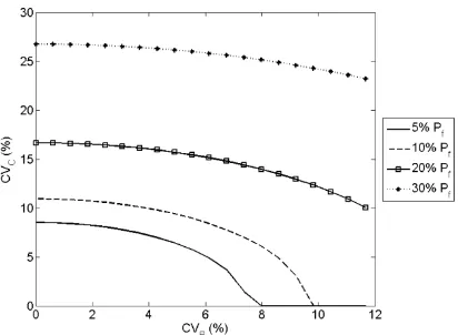
Fig. 5 illustrates the relationship between CVB and CVC
when Pf is fixed. The fixed Pf reflects the level of risk an
investor is willing to accept. In all levels of risk, increasing the fluctuation of future benefit should see investors decrease their exposure to cost uncertainty to maintain their acceptable risk level. That is, investors do not want to subject themselves to high uncertainties in both future inflow and outflow simultaneously. However, as an investor becomes more risk taking, for the same variation of benefit, an investor should be willing to accept a higher level of cost variation. This difference is more pronounced as benefit variation increases. For instance, comparing a risk averse investor (5% Pf) and a relatively risky investor (30% Pf) at
2% CVB, the difference in acceptable CVC is approximately
19% respectively. Increasing CVB to 8%, the difference
increases to 24%, with the risk averse investor not willing to accept any variations in cost. A small increase in variation in benefit has a bigger effect on risk averse investors.
0.0 0.5 1.0 1.5 2.0 2.5 3.0
‐3.0 ‐2.5 ‐2.0 ‐1.5 ‐1.0 ‐0.5 0.0
C'
B'
5 10 20
CVB(%)
Loss region
B < C
Safe region
[image:4.595.74.285.357.527.2]Fig. 5. At fixed levels of Pf, increasing CVB corresponds to decreases in CVC with µB = $1,628,865 and µC = $1,428,567.
IV. CONCLUSION
This paper has presented a theoretical framework in modeling risk and uncertainty using AFOSM reliability analysis in a cost-benefit setting. A life cycle analysis of a synthetic residential dwelling from an investor’s point of view has been applied with house price being treated as an uncertain variable. Autoregression has been introduced to forecast cost and benefit in future periods. The primary risk metric used was probability of loss. The focus was mainly on the effects of variations in future benefit or inflow, with variations in future cost or outflow also considered. It was found that probability of loss increases as the variation in benefit increases and the investment thus becomes riskier. Moreover, fluctuations in future benefits were viewed as positive risk when expected cost exceeded expected benefit, and investors should consider accepting higher variation in benefits by way of undertaking riskier decisions regarding future inflows. In contrast, fluctuations in future benefits were considered a negative risk when expected benefit exceeded expected cost, and investors should be inclined to be more risk averse and accept lower variations in future inflows. It was also identified that low levels of benefit variation does not exert a big influence on the probability of loss at low cost levels. In addition, increasing the fluctuation of future benefit should lead to investors decreasing their exposure to cost uncertainty regardless of an investors’ risk preference. Small increases in benefit variation have larger effects on the acceptable level of cost uncertainty for risk averse investors compared to risk taking investors.
The proposed approach is favored due to its computational efficiency over other uncertainty analysis methods such as commonly used Monte Carlo simulation. AFOSM addresses the problem of invariance that is evident in MVFOSM. Furthermore, there is potential for the framework to be extended to include non-monetary variables due to the unit-less conversion in determining β. Further works should investigate the incorporation of asymmetric behavior of investors to cost and benefit. The model could be further developed by considering correlation between multiple variables and non-normal properties of parameters. As the model is a flexible risk assessment tool with a holistic life cycle approach to financial aspects and potentially non-financial impacts. It could also be considered for application in other industry sectors to examine its scope and validity.
REFERENCES
[1] A. Haldar and S. Mahadevan, Probability, Reliability and Statistical Methods in Engineering Design. 2000, New York: John Wiley & Sons. [2] A. Ganji and L. Jowkarshorijeh, Advance first order second moment
(AFOSM) method for single reservoir operation reliability analysis: a case study.Stochastic Environmental Research and Risk Assessment, 2012. vol. 26, no. 1 pp. 33-42.
[3] M. Tichý, Applied Methods of Structural Reliability. Vol. 2. 1993, The Netherlands: Kluwer Academic Publishers.
[4] S. Adarsh and M. J. Reddy, Reliability analysis of composite channels using first order approximation and Monte Carlo simulations. Stochastic Environmental Research and Risk Assessment, 2013. vol. 27, no. 2 pp. 477-487.
[5] A. Mailhot and J. P. Villeneuve, Mean-value second-order uncertainty analysis method: application to water quality modelling.Advances in Water Resources, 2003. vol. 26, no. 5 pp. 491-499.
[6] J. Lai, L. Zhang, C. F. Duffield, and L. Aye, Economic Risk Analysis for Sustainable Urban Development: Validation of Framework and Decision Support Technique (Periodic style - Accepted for publication).Desalination and Water Treatment. no. to be published. [7] C. H. Nagaraja, L. D. Brown, and L. H. Zhao, An Autoregressive
Approach to House Price Modeling, 2009.
[8] D. M. Levine, D. Stephan, T. C. Krehbiel, and M. L. Berenson, Statistics for Managers Using Microsoft Excel. 3 ed, ed. T. Tucker. 2002, New Jersey: Pearson Education, Inc.
[9] E. Hunsinger, An expert-based stochastic population forecast for Alaska, using autoregressive models with random coefficients (working paper). 2010. no.