Numerical Solution of Fractional
Integro-differential Equation by Using Cubic
B-spline Wavelets
Khosrow Maleknejad, Monireh Nosrati Sahlan and Azadeh Ostadi
Abstract—A numerical scheme, based on the cubic B-spline wavelets for solving fractional integro-differential equations is presented. The fractional derivative of these wavelets are utilized to reduce the fractional integro-differential equation to system of algebraic equations. Numerical examples are provided to demonstrate the accuracy and efficiency and simplicity of the method.
Index Terms—fractional integro-differential equation, Ca-puto fractional differential equation, cubic B-spline wavelets, collocation method.
I. INTRODUCTION
T
HE objective of this paper is to introduce a comparative study to examine the performance of the Galerkin method via cubic B-spline wavelets in solving fractional integro-differential equations of the type:Dαy(t) =p(t)y(t) +f(t) + ∫ t
0
K(t, s)y(s)ds, (1)
0≤t≤1,
with initial condition
y(0) =y0, (2)
where the functionsf, p: [0,1]→RandK: [0,1]×[0,1]→
R are given and supposed to be sufficiently smooth and 0< α≤1.
The B-spline wavelets used in this work have compact support, vanishing moments and also they are semi or-thogonal. These properties causes many of the operational matrix entries be very small compared with the largest ones. Consequently, these elements can be set to zero with an opportune threshold technique without significantly affecting the solution.
The article is organized as follows: We begin by introducing some necessary definitions and mathematical preliminaries of the fractional calculus theory. Then cubic B-spline wavelets and function approximation by them are purposed which are required for establishing our results. Section 4 is devoted to applying the fractional differential of cubic B-spline scaling functions and wavelets for solving fractional integro-differential equation. In Section 5 the proposed method is applied to several examples. Also a conclusion is given in Section 6.
Manuscript received January 21, 2013; revised March 3, 2013. K. Maleknejad is with the Department of Mathematics, Iran University of Science and Technology, Narmak, Tehran 16846 13114, Iran. e-mail: [email protected]. Webpages.iust.ac.ir/Maleknejad
M. Nosrati Sahlan and A. Ostadi are with Iran University of Science and Technology. e-mails: [email protected] (Nosrati), [email protected] (Ostadi)
II. SOME PRELIMINARIES IN FRACTIONAL CALCULUS
In this section we briefly present some definitions and results in fractional calculus for our subsequent discussion [1]. The fractional calculus is the name for the theory of integrals and derivatives of arbitrary order, which unifies and generalizes the notions of integer-order differentiation and n-fold integration [1]-[2]. There are various definitions of fractional integration and differentiation, such as Grunwald-Letnikov and Riemann-Liouville’s definitions.
The Riemann-Liouville derivative has certain disadvantages when trying to model real-world phenomena with fractional differential equations. The reason for adopting the Caputo definition, as pointed by [3], is as follows: to solve differ-ential equations (both classical and fractional), we need to specify additional conditions in order to produce a unique solution. For the case of the Caputo fractional differential equations, these additional conditions are just the traditional conditions, which are akin to those of classical differential equations and are therefore familiar to us. In contrast, for the Riemann-Liouville fractional differential equations, these additional conditions constitute certain fractional derivatives (and/or integrals) of the unknown solution at the initial point
x= 0, which are functions ofx. These initial conditions are not physical; furthermore, it is not clear how such quantities are to be measured from experiment, say, so that they can be appropriately assigned in an analysis. For more details see [4]. Therefore, we shall introduce a modified fractional differential operatorDαproposed by Caputo in his work on the theory of viscoelasticity [5].
Definition: The Caputo definition of the fractional-order derivative of functionf : [a, b]→R is defined as:
Dαf(x) = 1 Γ(n−α)
∫ x
0
f(n)(t)
(x−t)α+1−ndt, (3) n−1< α≤n, n∈N
whereαis the order of the derivative andnis the smallest integer greater than α. For the Caputo derivative we have [6]:
DαC= 0, (C is a constant),
Dαxβ= 0, β∈N, β <⌈α⌉, Dαxβ= Γ(β+ 1)
Γ(β+ 1−α)x
β−α,
β∈N, β≥ ⌈α⌉or β∈R−N0, β >⌊α⌋,
toαandN0= 0,1,2, ....
For the Laplace transformation of f(x)we have:
L(Dαf(x)) =sαLf(x)−
n−1
∑
j=0
sα−1−jf(j)(0). (4)
It is clear that for α ∈ N the Caputo differential operator coincides with the usual differential operator of an integer order. Similar to the integer-order differentiation, the Caputo fractional differentiation is a linear operator:
Dα(λf(x) +µg(x)) =λDαf(x) +µDαg(x),
where λ and µ are constants. In the present work, the fractional derivatives are considered in the Caputo sense.
III. CUBICB-SPLINE SCALING AND WAVELET FUNCTIONS
The general theory and basic concepts of the wavelet theory and MRA are given in [7]-[12].
Wavelets and scaling functions are defined on the entire real line so that they could be outside of the integration domain. This behavior may require an explicit enforcement of the boundary conditions. In order to avid this occurrence, semiorthogonal compactly supported spline wavelets, con-structed for the bounded interval[0,1], have been taken into account in this paper. These wavelets satisfy all the properties verified by the usual wavelets on the real line.
Definition: Letm andnbe two positive integers and
a=x−m+1=. . .=x0< . . . < xn =. . .=xn+m−1=b,
be an equally spaced knots sequence. The functions
Bm,j,X(x) =
x−xj xj+m−1−xj
Bm−1,j,X(x)
+ xj+m−x
xj+m−xj+1
Bm−1,j,X(x),
j=−m+ 1, . . . , n−1,
and
B1,j,X(x) =
{
1 x∈[xj, xj+1),
0 otherwise,
are called cardinal B-spline functions of orderm≥2for the knot sequenceX ={xi}in=+−mm−+11 , andSupp[Bm,j,X(x)] =
[xj, xj+m]
∩ [a, b].
For the sake of simplicity , suppose
[a, b] = [0, n], xk =k, k= 0, ..., n.
The Bm,j,X = Bm(x − j), j = 0, ..., n − m,
are interior B-spline functions, while the remaining
Bm,j,X, j=−m+ 1, ...,−1andj =n−m+ 1, ..., n−1are
boundary B-spline functions, for the bounded interval[0, n]. Since the boundary B-spline functions at 0 are symmetric reflections of those atn, it is sufficient to construct only the first half functions by simply replacingxwithn−x. By considering the interval [a, b] = [0,1], at any level
j ∈ Z+, the discretization step is 2−j and this generates
n= 2j number of segments in[0,1]with knot sequence
X(j)=
x(−jm)+1=...=x(0j)= 0,
x(kj)= 2kj k= 1, ..., n−1,
x(nj)=...=x (j)
n+m−1= 1.
Letj0 be the level for which
2j0 ≥2m−1,
for each levelj ≥j0 the scaling functions of order m can be defined as follows:
φ(m,kj) (x) =
Bm,j0,k(2
j−j0x)
k=−m+ 1, ...,−1
Bm,j0,2j−m−k(1−2
j−j0x)
k= 2j−m+ 1, ...,2j−1
Bm,j0,0(2
j−j0x−2−j0k)
k= 0, ...,2j−m.
And the two-scale relation for them-order semi orthogonal compactly supported B-wavelet functions are defined as follows:
ψm,j,i−m=
2i+2∑m−2
k=i
qi,kBm,j,k−m , i= 1, ..., m−1, (5)
ψm,j,i−m=
2i+2∑m−2
k=2i−m
qi,kBm,j,k−m, i=m, ..., n−m+ 1,
(6)
ψm,j,i−m=
n+i∑+m−1
k=2i−m
qi,kBm,j,k−m , i=n−m+ 2, ..., n,
(7) whereqi,k=qk−2i.
Hence, there are2(m−1)boundary wavelets and(n−2m+ 2) inner wavelets in the boundary interval[a, b]. Finally by considering the levelj withj≥j0, the B-wavelet functions in[0,1]can be expressed as follows:
ψm,j,i(x) =
ψm,j0,i(2
j−j0x)
i=−m+ 1, ...,−1
ψm,2j−2m+1−i,i(1−2j−j0x)
i= 2j−2m+ 2, ...,2j−m ψm,j0,0(2
j−j0x−2−j0i)
i= 0, ...,2j−2m+ 1.
(8)
The scaling functionsφ(m,kj) (x), occupymsegments and the
wavelet functionsψm,i(j)(x)occupy2m−1 segments. Therefore the condition2j ≥2m−1, must be satisfied in order to have at least one inner wavelet.
Cubic B-spline scaling functionφ4(x)is given by:
φ4(x) = 1 6 4 ∑ k=0 ( 4 k )
(−1)k(x−k)3+=
1 6x
3 x∈[0,1)
1 6(−3x
3+ 12x2−12x+ 4) x∈[1,2) 1
6(3x
3−24x2+ 60x−44) x∈[2,3) 1
6(4−x)
3 x∈[3,4)
0 otherwise,
(9)
where
xn+= {
xn , x >0
0 1 2 3 4 5
-0.1
[image:3.595.46.542.46.836.2]0.0 0.1 0.2 0.3 0.4 0.5 0.6 0.7
Fig. 1. Two scale relation ofφ4(x)
And its two-scale dilation equation defined as follows:
φ4(x) =
4
∑
k=0
1 8
( 4
k
)
φ4(2x−k). (10) Fig 1 shows the two scale relation of cubic B-spline scaling functions. In this section, the scaling functions used in this work, forj0=j= 3 andm= 4, are reported :
Boundary scalings
Three left boundary cubic B-spline scaling functions are constructed by the following formula:
φ(3)4,k(x) =φ4(8x−k).χ[0,1](x), (11) k=−3,−2,−1,
and for other levels of j, we have:
φ(4j,k)(x) =φ(3)4,k(2j−3x), (12)
k=−3,−2,−1, j= 4,5, . . .·
left and right boundary scaling functions are symmetric with respect to 0, so right boundary scalings are constructed by:
φ(3)4,5(x) =φ4(3),−1(1−x), (13)
φ(3)4,6(x) =φ4(3),−2(1−x), (14)
φ(3)4,7=φ(3)4,−3(1−x), (15) and for other levels of j, we have:
φ(4j,2)j−k−3(x) =φ
(3) 4,k(2
j−3x),
(16)
k=−3,−2,−1, j= 4,5, . . .·
Inner scalings
Five inner cubic B-spline scaling functions are constructed by the following formula:
φ(3)4,k(x) =φ4(8x−k).χ[0,1](x), (17) k= 0,1,2,3,4,5,
and for other levels of j, we get:
φ(4j,k)(x) =φ4(3),k(2j−3x−k),
k= 0,1, ...,2j−4, j= 4,5, . . .· (18) Two scale delation equationfor cubic B-spline wavelet is given by:
ψ4(x) =
10
∑
k=0
(−1)k
8
4
∑
l=0
( 4
l
)
φ8(k−l+ 1)φ4(2x−k).
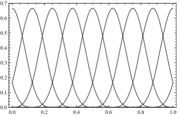
0.0 0.2 0.4 0.6 0.8 1.0
[image:3.595.78.263.52.174.2]0.0 0.1 0.2 0.3 0.4 0.5 0.6 0.7
Fig. 2. Boundary and inner scaling functions
0.0 0.2 0.4 0.6 0.8 1.0
-0.2
[image:3.595.336.520.53.171.2]-0.1 0.0 0.1 0.2
Fig. 3. Boundary and inner wavelets
Other inner and boundary wavelets are made similarly by equations 5-8 [13].
Figures 2 and 3 show the boundary and inner scaling and wavelet functions for cubic B-spline wavelet.
A. Function approximation
A functionf(x)defined over[0,1]may be approximated by cubic B-spline wavelets as:
f(x) =
2j∑0−1
i=−3
cj0,iφj0,i(x) + ∞
∑
k=j0
2k−4
∑
j=−3
dk,jψk,j(x), (19)
where φj0,i and ψk,j are scaling and wavelets functions,
respectively. If the infinite series in equation 19 is truncated, then it can be written as:
f(x)≃
i=2∑j0−1
i=−3
cj0,iφj0,i(x) +
ju
∑
k=j0
2k−4
∑
j=−3
dk,jψk,j(x),
or
f(x)≃CTΥ(x), (20) whereC andΥare (2(ju+1)+ 3) column vectors given by
C=(cj0,−3, ..., cj0,2j0−1, dj0,−3, ..., dju,2ju−4
)T
, (21)
Υ =(φj0,−3, ..., φj0,2j0−1, ψj0,−3, ..., ψju,2ju−4
)T , (22)
with
cj0,i=
∫ 1
0
f(x) ˜φj0,i(x)dx , i=−3, ...,2
j0−1,
dk,j =
∫ 1
0
f(x) ˜ψk,j(x)dx
k=j0, ..., ju , j=−3, ...,2ju−4,
and φ˜j0,i and ψ˜k,j are dual functions of φj0,i, i =
−3, ...,2j0−1 andψ
[image:3.595.337.517.204.317.2]respectively. These can be obtained by linear combinations of φj0,i andψk,j.
Let
φ(x) = (
φ(3)4,−3(x), φ(3)4,−2(x), ..., φ(3)4,7(x) )T
, (23)
ψ(x) = (
ψ(3)4,−3(x), ..., ψ4(3),4(x), ..., ψ(ju)
4,2ju−4(x)
)T , (24)
and
∫ 1
0
φ(x)φT(x)dx=P1, (25)
∫ 1
0
ψ(x)ψT(x)dx=P2, (26)
whereP1andP2 are11×11and(2ju+1−8)×(2ju+1−8)
matrices, respectively. Suppose φ˜(x) andψ˜(x) are the dual functions of φ(x)andψ(x), given by
˜
φ(x) = (
˜
φ(3)4,−3(x),φ˜(3)4,−2(x), ...,φ˜(3)4,7(x) )T
, (27)
˜
ψ(x) = (
˜
ψ(3)4,−3(x), ...,ψ˜4(3),4(x), ...,ψ˜(ju)
4,2ju−4(x)
)T . (28)
Using equations 23-24, 27 and equation 28 we have ∫ 1
0
˜
φ(x)φT(x)dx=I11,
∫ 1
0
˜
ψ(x)ψT(x)dx=I2ju+1−8.
whereI11andI2ju+1−8are11×11and(2ju+1−8)×(2ju+1−
8) identity matrices, respectively. So we get
˜
φ=P1−1φ, ψ˜=P2−1ψ.
Thus, the dual function ofΥcan be constructed as:
˜
Υ(x) =P−1Υ(x),
where
P= (
P1 P2
)
.
Now, we found a bound for wavelet coefficients.
Theorem 1: [13] We assume thatf ∈C4[0,1]is represented
by cubic B-spline wavelets as 20, where ψ has4 vanishing moments, then
|dj,k| ≤αβ
2−5j
4! , (29)
where
α= max|f(4)(t)|t∈[0,1], β=
∫ 1
0
|x4ψ4˜ (x)|dx.
Theorem 2: [13] Consider the previous theorem assume that
ej(x)be error of approximation inVj, then
|ej(x)|=O(2−4j). (30)
As is shown in equation 30, the order of the error depends on the level j. Obviously, for larger level of j, the error of approximation will be smaller.
IV. NUMERICALIMPLEMENTATION
Since all the boundary and inner B-spline scaling functions and wavelets are composed by cardinal B-spline function of orderm= 4, if the analytical expressions ofDαφ4(x), is obtained, those of the boundary and inner B-spline scaling functions and wavelets can be naturally achieved.
Theorem 3: Form∈N andm < α≤m+ 1, n >0, x >
0, a >0, b≥0, ifα≤nor α∈N, then:
Dα(ax−b)n+=aα Γ(n+ 1)
Γ(n+ 1−α)(ax−b)
n−α
+ . (31)
Proof: Let
f(x) =xn+, g(x) =f(ax−b) = (ax−b)n+,
then the Laplace transform off(x)is:
F(s) = ∫ ∞
0
e−sxf(x)dx=Γ(n+ 1)
sn+1 ,
by the property of the Laplace transform, Laplace transform ofg(x)is:
G(s) = ∫ ∞
0
e−sxg(x)dx=1
ae −b
asF(s
a),
From the property of fractional derivative equation 6, we can obtain:
L(Dα(ax−b)+n)=L(Dαg(x)) =
sαG(s)−
m
∑
j=0
sα−1−jg(j)(0) =
an Γ(n+ 1)
Γ(n+ 1−α)L [(
x−b a
)n−α
+
] =
aα Γ(n+ 1)
Γ(n+ 1−α)L [
(ax−b)n+−α]. (32) From the uniqueness of Laplace transform, we get:
Dα(ax−b)n+=aα Γ(n+ 1)
Γ(n+ 1−α)(ax−b)
n−α + .
Now, we derive the analytical expression ofDαφ4(x). Theorem 4:
Dαφ4(x) = 1 Γ(4−α)
4
∑
k=0
( 4
k
)
(−1)k(x−k)3+−α. (33) Proof: By substituting 9 in 31, proof is completed.
So by the fractional derivative of φ4(x) we can obtain
the fractional derivative of boundary scaling functions as follows:
Dαφ(3)4,k(x) =Dαφ4(8x−k).χ[0,1](x) =
( 8α
Γ(4−α)
4
∑
i=0
( 4
i
)
(−1)i(8x−k−i)3−α )
.χ[0,1](x),
(34)
K=−3,−2,−1.
And for other levels ofj, we get:
Dαφ(4j,k)(x) =Dαφ(3)4,k(2j−3x) = (
2jα
Γ(4−α)
4
∑
i=0
( 4
i
)
(−1)i(2jx−k−i)3−α )
.χ[0,1](x),
K=−3,−2,−1, j= 4,5, . . . .
By the symmetry property of B-spline scaling functions, the fractional derivative of right boundary scaling functions are constructed similarly:
Dαφ(3)4,k(x) =Dαφ(3)4,4−k(x). k= 5,6,7. (36)
Fractional derivative of inner scaling functions can be for-mulated as follows:
Dαφ(3)4,k(x) =Dαφ4(8x−k).χ[0,1](x) =
( 8α
Γ(4−α)
4
∑
i=0
( 4
i
)
(−1)i(8x−k−i)3−α )
.χ[0,1](x),
(37)
K= 0,1, ...,5.
And for other levels ofj, we get:
Dαφ(4j,k)(x) =Dαφ(3)4,k(2j−3x−k) = (
2jα
Γ(4−α)
4
∑
i=0
( 4
i
)
(−1)i(2jx−k−i)3−α )
.χ[0,1](x),
(38)
K= 0,1, . . . ,2j−4, j= 4,5, . . . .
The fractional derivative of B-spline wavelets are made similarly. Therefore the fractional derivative of Υ(t) is as follows:
DαΥ(t) =(Dαφj0,−3(t), ..., D
αψ
ju,2ju−4(t)
)T
, (39)
Now for solving the equation 1, the fractional derivative of unknown function is approximated by cubic B-spline wavelets as:
Dαy(t) =Dα(CTΥ(t)) =CTDαΥ(t), (40)
substituting the current equation in equation 1, we have:
CTDαΥ(t) =CTp(t)Υ(t) +f(t) +CT
∫ t
0
K(t, s)Υ(t)dt,
(41) To find the solutiony(t), we collocate the equation 41 in
ti = i
2ju+1+ 2, i= 0,1, . . . ,2
ju+1+ 2,
so the fractional integro-differential equation transform to some algebraic linear equation that can be solved by some iteration method.
The limits of integrations in equation 41 range from zero to one; the actual integration limits are much smaller because of the finite supports of the semiorthogonal scaling functions and wavelets. Moreover, a lot of integrals in equation 41 become zero due to the semiorthogonality and vanishing mo-ments properties of the wavelet functions. So using cubic B-spline wavelets, a sparse system of equations can be obtained from fractional integro-differential equation. Therefore, by using present method, we can economize in computational time and memory requirement.
TABLE I
EXACT AND NUMERICAL SOLUTION OF EXAMPLE1 xi ju= 4 ju= 5 Method of [14] Exact
0 0.00003 0.000000 0.00056 0
0.2 0.0080371 0.00800 0.008694 0.008 0.4 0.064024 0.064000 0.64098 0.064 0.6 0.216084 0.216000 0.216058 0.216 0.8 0.512043 0.512000 0.512583 0.512
1 1.000028 1.000000 1.000064 1
TABLE II
EXACT AND NUMERICAL SOLUTION OF EXAMPLE2 xi ju= 4 ju= 5 Method of [14] Exact
0 0.000286 0.000000 0.000357 0.0 0.2 0.240010 0.240000 0.240035 0.24 0.4 0.560087 0.560000 0.560093 0.56 0.6 0.960053 0.960000 0.960026 0.96 0.8 1.440081 1.440000 1.440073 1.44 1 2.000617 2.000000 2.001013 2
V. ILLUSTRATIVE EXAMPLES
In this section, for showing the accuracy and efficiency of the described method we present some examples.
Example 1: Consider the following fractional integro-differential equation:
y(34)(t) =
(
−t2et
5 )
y(t) + 6
4
√
t9
Γ(3.25)+ ∫ t
0
etsy(s)ds,
with the initial condition y(0) = 0 and the exact solution
y(t) =t3.
The solution for y(t) is obtained by the method in Section 5 at the octave level j0 = 3 and at the levelsju = 4 and
5. In Table I, we present exact and approximate solutions of Example 1 in some arbitrary points. As proved perviously, the error at the level ju = 5 is smaller than the error at ju= 4.
Example 2: Consider the following fractional integro-differential equation:
y(12)(t) = (cos(t)−sin(t))y(t) +f(t) +
∫ t
0
tsin(s)y(s)ds,
with the initial conditiony(0) = 0andf(t)is chosen such that the exact solution of equation isy(t) =t2+t.
The solution for y(t) is obtained by the method in Section 5 at the octave levelj0= 3 and at the levelsju= 4 and 5.
In Table II, we present exact and approximate solutions of Example 2 in some arbitrary points. As proved perviously, the error at the level ju = 5 is smaller than the error at ju= 4.
VI. CONCLUSION
with little additional work. Further research along these lines is under progress and will be reported in due time.
REFERENCES
[1] A. A. Kilbas, H. M. Srivastava and Juan. J. Trujillo, “Theory and Applications of Fractional Differential Equations,” North Holland Mathematics Studies, vol. 204, Elsevier Science, B.V., Amsterdam, 2006.
[2] S. Das,Functional Fractional Calculus for System Identification and Controls, Springer, New York, 2008.
[3] S. Momani and M. A. Noor, “Numerical methods for fourth-order fractional integro-differential equations,” Appl. Math. Comput., vol. 182, pp. 754-760, 2006.
[4] I. Podlubny, “Geometric and physical interpretation of fractional integration and fractional differentiation,”Fract. Calculus Appl., Anal. vol. 5, pp. 367-386, 2002.
[5] M. Caputo, “Linear models of dissipation whose Q is almost frequency independent. Part II,”J. Roy Austral. Soc., vol. 13, pp. 529-539, 1967. [6] K. Diethelm, N. J. Ford, A. D. Freed and Yu. Luchko, “Algorithms for the fractional calculus: A selection of numerical methods,”Comput. Methods Appl. Mech. Eng., vol. 194, pp. 743-773, 2005.
[7] C. Chui,An introduction to wavelets,New york: Academic press, 1992. [8] I. Daubechies,Ten lectures on wavelets, Philadelpia, PA; SIAM, 1992. [9] G. Strang and T. Nguyen,Wavelets and filter banks, Cambridge, MA:
Wellesley-Cambridge, 1997.
[10] L. Telesca, G. Hloupis, I. Nikolintaga and F. Vallianatos, “Temporal patterns in southern Aegean seismicity revealed by the multiresolution wavelet analysis,”Commun. Non. Sci. Num. Simul., vol. 12, pp. 1418-1426, 2007.
[11] C. Chui,Wavelets: a mathematical tool for signal analysis, Philadelpia, PA: SIAM, 1997.
[12] S. G. Mallat, “A theory for multiresolution signal decomposition: The wavelet representation, IEEE Trans,”Pattern Anal. Mach. Intell., vol. 11, pp. 674-693, 1989.
[13] K. Maleknejad, K. Nouri and M. Nosrati Sahlan, “Convergence of approximate solution of nonlinear Fredholm-Hammerstein integral equations,”Commun. Nonlinear. Sci. Num. Simul., vol. 15, no. 6, pp. 1432-1443, 2010.