Using geodesic space density gradients for network community detection

warwick.ac.uk/lib-publications

Original citation:

Mahmood, Arif, Small, Michael, Al-Maadeed, Somaya and Rajpoot, Nasir M. (Nasir

Mahmood). (2017) Using geodesic space density gradients for network community

detection. IEEE Transactions on Knowledge and Data Engineering, 294 (4). pp. 921-935.

Permanent WRAP URL:

http://wrap.warwick.ac.uk/84012

Copyright and reuse:

The Warwick Research Archive Portal (WRAP) makes this work by researchers of the

University of Warwick available open access under the following conditions. Copyright ©

and all moral rights to the version of the paper presented here belong to the individual

author(s) and/or other copyright owners. To the extent reasonable and practicable the

material made available in WRAP has been checked for eligibility before being made

available.

Copies of full items can be used for personal research or study, educational, or not-for profit

purposes without prior permission or charge. Provided that the authors, title and full

bibliographic details are credited, a hyperlink and/or URL is given for the original metadata

page and the content is not changed in any way.

Publisher’s statement:

“© 2017 IEEE. Personal use of this material is permitted. Permission from IEEE must be

obtained for all other uses, in any current or future media, including reprinting

/republishing this material for advertising or promotional purposes, creating new collective

works, for resale or redistribution to servers or lists, or reuse of any copyrighted component

of this work in other works.”

A note on versions:

The version presented here may differ from the published version or, version of record, if

you wish to cite this item you are advised to consult the publisher’s version. Please see the

‘permanent WRAP URL’ above for details on accessing the published version and note that

access may require a subscription.

1

Using Geodesic Space Density Gradients for

Network Community Detection

Arif Mahmood, Michael Small, Somaya Ali Al-Maadeed, and Nasir Rajpoot

Abstract—Many real world complex systems naturally map to network data structures instead of geometric spaces because the only available information is the presence or absence of a link between two entities in the system. To enable data mining techniques to solve problems in the network domain, the nodes need to be mapped to a geometric space. We propose this mapping by representing each network node with its geodesic distances from all other nodes. The space spanned by the geodesic distance vectors is the geodesic space of that network. Position of different nodes in the geodesic space encode the network structure. In this space, considering a continuous density field induced by each node, density at a specific point is the summation of density fields induced by all nodes. We drift each node in the direction of positive density gradient using an iterative algorithm till each node reaches a local maximum. Due to the network structure captured by this space, the nodes that drift to the same region of space belong to the same communities in the original network. We use the direction of movement and final position of each node as important clues for community membership assignment. The proposed algorithm is compared with more than ten state of the art community detection techniques on two benchmark networks with known communities using Normalized Mutual Information criterion. The proposed algorithm outperformed these methods by a significant margin. Moreover, the proposed algorithm has also shown excellent performance on many real-world networks.

Index Terms—Complex Networks, Community Detection, Geodesic Space, Geodesic Distance, Density Field Gradients

F

1

I

Many real world complex systems such as social networks on facebook and twitter, the internet and the web of hyper-links, connections between different components in an electric circuit and interactions of neural cells directly map to network data structures instead of geometric spaces. Therefore, network the-oretic algorithms have often been used to analyze the structure of the underlying systems to study various network aspects such as interactions within the network, change propagation, edge and node density variations and resilience to targeted or random attacks. Often the edge and the node distribution is inhomogeneous in real-world networks resulting in node groups with high number of intra-group and low number of inter-group edges. These groups are referred to as communities and play an important role in the understanding of the structure of complex systems [37], [3].

Communities are the groups of entities in a network which share common attributes and often exhibit similar behavior. Com-munity detection has the potential to solve many real world challenges such as identification of communities of clients having similar interests help in improving the service standards. The online community structure within social networks influences information propagation across the globe. The network of pas-sengers traveling across countries define the spread of diseases across continents. A community of health workers and the patients

● A. Mahmood and S A Al-Maadeed are with the Department of Computer

Science and Engineering, College of Engineering, Qatar University, Doha,

Qatar. E-mails:{arif.mahmood, s alali}@qu.edu.qa,

● M. Small is with the School of Mathematics and Statistics and the Complex

Data Modelling Group, The University of Western Australia, WA 6009. Michael is also with Mineral Resources, CSIRO, Kensington, WA 6151. E-mail: [email protected],

● Nasir Rajpoot is with the Department of Computer Science, University of

Warwick, UK. E-mail: [email protected].

Manuscript received January 2016.

they handled share a level of exposure to the disease proportional to the intra-community links. Such communities are important for isolating possible carriers of contagious diseases such as the Ebola virus. Thus identification of network communities is an important topic across a number of research areas [14], [16].

Most existing community detection algorithms [8], [12], [18], [38], [42], [45], [46], [48] are graph theoretic and directly operate on the adjacency matrix. Most graph theoretic algorithms lack the ability to detect accurate community boundaries if the average difference between the internal and the external node degree does not exceed a strictly positive threshold [44]. Most of these methods use modularity [38], [17] as the quality index of a community. It has been observed that modularity maximization algorithms fail to identify communities smaller than a particular size even in cases when communities are well-defined [29]. The proposed community detection algorithm is fundamentally different from existing techniques as it is not based on modularity maximization. We experimentally observe that our proposed algorithm can detect communities at multiple resolutions. Also the detected community boundaries are more accurate even if the external node degree is the same as internal or even larger in some cases.

The proposed Geodesic Density Gradient (GDG) algorithm

Geodesic Distance at

All Pairs

Final Node Positions

After Iterative

Drifting

Linear Clustering

Complex Network Mapped to Geometric Space Estimating Maximum Density Regions Network with Community Labels

Step 1 Step 2 Step 3

Fig. 1. Proposed algorithm has three main steps: for a given network geodesic distance at all pairs is computed and each node is represented by the corresponding vector of distances. In the geometric space, each node is drifted towards the local density maximum following a positive density gradient. A linear clustering algorithm is used to find an estimate of each maximum density region. All nodes drifting towards a particular region are assigned the same community label.

structure as recently shown by Mahmood and Small [35]. The space spanned by the geodesic distance vectors of a network is the geodesic space of that network. Distribution of nodes in the geodesic space encodes the network structure. Distance between two nodes in this space depends on the global position of these nodes in the network. The global network structure consists of global communities, while in many cases local network structure is also important to determine accurate local community boundaries. We propose a distance which incorporates both the global as well as local network structure for better discrimination between nodes belonging to the different communities especially on the community boundaries.

The motivation for the next step is to bring closer the nodes belonging to the same community, and move away the nodes belonging to the different communities. Purpose is compactness of communities and larger inter community gaps which will improve community detection performance. For this purpose, we consider each node in the geodesic space inducing a density field which is maximum at the node position and reduces as the distance increases. Density fields induced by all nodes get superimposed and therefore in certain regions of the space density becomes more compared to the other regions. This density distribution depends on the node distribution in the space which depends upon the network structure. Thus if the network structure varies, density distribution in geodesic space will also vary. For each node, we compute the direction of maximum positive density gradient and drift the node in that direction. Considering only one node at a time, the algorithm drifts all nodes one by one and then starts from the first node once again. The process is repeated until most of the nodes converge to regions with minimal density variation. These uniform density regions are also local maximum of the density field. It is because nodes have followed positive density gradients to reach these regions. The path followed by each node from its original position to the final position is a trajectory in the geodesic space (Figure 2). We observe that the nodes converging towards the same local maximum density region belongs to the same community in the original network. It is because of the network structure encoded in the geodesic space, the community structure translates into cluster structure. Our experiments show that the proposed algorithm can resolve communities at different resolutions much better than the traditional methods based on modularity optimization.

As a post processing step, clustering is required to be per-formed. It is because all nodes belonging to the same community do not converge to exactly the same position in the geodesic space. As a node drifts closer to a uniform density region, the density gra-dient gradually reduces to zero. Also the distribution of the density

a) Dolphins, K=6 b)karate, K=4

(a)

(b)

(c) (d)

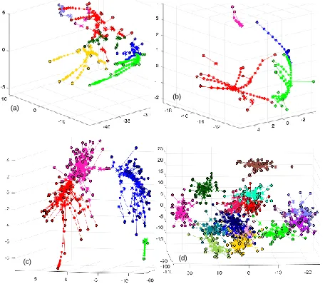
c) Jazz d) synthetic network Fig. 2. In consecutive iterations of the step 2 of the proposed algorithm, nodes drift in the direction of positive density gradient and converge towards local density maximum regions. Initial position of a node is shown as circle and final position as ‘∗’. Each community is shown in a different color. (a) Dolphins Network [33], [34](b) Zachary Karate Club [50] (c) Jazz Bands Network [19] (c) LFR Benchmark [31] with 500 nodes and 13 communities.

gradient is not uniform around a maximum in the geodesic space causing nodes drifting from different directions to be stopped at different positions. By using a simple approach based on the k-means clustering algorithm we find clusters of nodes. A challenge with using the k-means algorithm is that it requires the number of clusters (unknown to us) as an input parameter. We solve this problem by varying the number of clusters and by observing the variation of clustering error derivative we can estimate an appropriate number of clusters in the network (see Figures 6 & 7). Note that other clustering algorithms such as DBSCAN [13] and OPTICS [2] do not require the number of clusters but do require other input parameters including the maximum distance

(), and the minimum number of points (M inP ts). There is no

3

−120

−100

−80

−30 −20

−10 0

10 20

30 −20 −10 0 10 20 30

Fig. 3. An LFR benchmark network with 500 nodes, 2500 links used to demonstrate the proposed algorithm. Each node is represented by a 500 dimensional geodesic distance vector. For the purpose of visualization each node is projected on the three principal components using PCA. A 3D view of the network is rotated to clearly show all planted communities using different random colors.

−110−100−20−90 −15 −10 −5 0 5 10 15 20 −15 −10 −5 0 5 10 15 20 25

Fig. 4. The same network in Figure 3 after nodes have been iteratively drifted towards the local maximum density regions in the geodesic space. Communities have become more compact and inter-community distances have increased. Due to this step, significant performance gain is obtained compared to direct application of clustering techniques on the network shown in Figure 3. Using the proposed algorithm, we were able to find all 16 communities without any error.

increased making the community boundaries more distinct. This is one of the main reasons why we were able to obtain a better performance than the other algorithms which do not use this step. On the converged network, we applied k-means algorithm. As the number of clusters increased in the k-means algorithm, the

clustering error decreased at a larger rate tillk=16. Beyond that

the rate of decrease of clustering error was quite small. The 16 identified communities are shown in Figure 4 using different ran-dom colors. On the same network modularity maximization was also applied by varying the number of communities. Maximum modularity of 0.859 was obtained for 12 communities shown in Figure 5 using random colors. At least three communities contain visible sub-groups. This experiment shows that despite obvious structure, modularity maximization was not able to resolve all communities. In contrast, in this example, our proposed algorithm has accurately detected all communities without suffering from the resolution limit.

−110 −100

−9020 15 10 5 0 −5 −10 −15 −20

−15 −10 −5 0 5 10 15 20 25

Fig. 5. For network of Figure 3 maximum modularity was obtained for 13 communities shown by different random colors. Each of the red, green and blue community has two groups of nodes. Despite an obvious community structure, modularity maximization failed to resolve all communities.

The idea of drifting nodes towards local density maxima in geodesic space is conceptually similar to the Mean Shift algo-rithm [7], [9]. However, to the best of our knowledge no similar algorithm has yet been applied to the problem of community detection in complex networks. In this direction, our contributions are several including a suitable distance for community detection in the geodesic space (Section 3.1), derivation of the estimate of the new node position using the proposed distance measure (Sec-tion 3.2), and estima(Sec-tion of the maximum density regions (Sec(Sec-tion 3.3). We also propose a technique to estimate suitable number of communities in a given network based on clustering error derivative (Section 3.4). Our experimental results will demonstrate the effectiveness of the proposed algorithm (Section 4). In the next section we give a brief overview of the related work.

2

R

W

We broadly arrange the important existing community detection methods in two groups. The methods in the first group use graph attributes to find communities. Methods in the second group map a network to a geometric space and then use pattern recognition techniques for community detection. Our proposed algorithm comes under the second group.

2.1 Graph Theoretic Algorithms

In this group of algorithms, network communities have been de-fined in a number of ways. S. V. Dongen considered a community to be a group of nodes if visited by a random walk, the walk will likely not leave the group until most of its vertices have been visited. He proposed Markov Cluster algorithm [48] based on the idea of current flow in the graph. If natural groups are present in the graph, then the current across group borders will be small thus revealing group structure in the graph.

triangles. Edges connecting different groups have low clustering coefficient and are removed first.

Girvan and Newman [18], [38] proposed a community detec-tion algorithm (GN) based on the concept of edge betweenness which is the number of shortest paths that run along an edge. The edge with highest betweenness is removed and shortest paths are recomputed each time. Clauset et al.[8] proposed a fast greedy modularity optimization algorithm which is very efficient on sparse graphs with hierarchical structure. Blondel et al.[4] proposed a modularity optimization based fast heuristic algorithms for community structure extraction in large networks.

Palla et al. [42] defined a community as a union of all k

-cliques (complete subgraphs of sizek) that can be reached from

each other through a series of adjacentk-cliques (where adjacency

means sharingk−1nodes). Their method first locates all cliques

of the network and then finds the communities by carrying out a standard component analysis of the cliqueclique overlap. Chen and Saad [6] define communities as dense subgraphs.

Donetti and Munoz [12] have proposed DM algorithm which is spectral clustering for community detection. First a few eigenvec-tors of the network Laplacian matrix are computed and then based on Euclidean or angular distance existing algorithms are used to find clusters. Rosvall and Bergstrom has proposed an information-theoretic framework for resolving community structure in complex networks [47] known as Infomap. A network is divided into small modules such that Minimum Description Length (MDL) is minimized.

2.2 Mapping Networks to Geometric Spaces

Finding communities in complex networks by mapping to

geo-metric spaces has not been well investigated. Nishikawaet al[41]

used 28 node properties for feature space representation. Twenty of these properties are the eigenvector coefficients of the Laplacian and the normalized Laplacian matrices. Their method mainly leverages the strength of spectral clustering which maps data from nonlinear manifolds to linear space where data can be grouped by using k-means algorithm. Moreover, despite significant difference in the meaning of different features, the 28 dimensional feature vector is projected to random 2D space and the user is required to manually mark the clusters. The user input over different 2D views is combined to infer the community structure. In contrast to this approach, we represent a node with a feature vector containing the same type of distance from all other nodes in the network. Thus our approach is purely distance based and does not include node properties such a node degree or centrality which are not relevant to the notion of distance.

Jinet al [26] defined a distance function between two nodes based on the geometric mean of the costs of all paths between those nodes. Each node is assigned a density value as the sum of exponentially decaying influence functions. The node with maximum density value is selected to be the density-attractor and the nodes directly connected to it with lower density values are considered as the density-attracted. The embedding space is dis-crete considering only two nodes at a time. Another density based heuristic approach was proposed by Gong et al [20]. Similarity between two nodes was defined as the ratio of cardinality of the intersection to the union of the neighbors of the two nodes. All nodes in the neighborhood of a node with similarities larger than a threshold parameter are considered as one group. Recently

Deriteiet al[11] represented distance between two nodes based

on the edge-clustering coefficient and used Voroni diagrams for community detection. To the best of our knowledge, none of these algorithms have used the drifting of nodes towards positive density gradients to increase compactness of communities and improved discrimination by increased inter community distances as we propose before the clustering step. This is one of the main reasons our algorithm was able to achieve very good performance in almost all test cases.

In all of the existing approaches [11], [26], [20] network to geometric space mapping is considered for only two nodes at a time while the positions of the rest of the nodes in the geometric space are ignored. Since the assumed spaces are not continuous, therefore these are also not directly differentiable. None of these approaches are capable to represent complete network in the embedding space at the same time with an exception of Nishikawa

et al[41]. They were able to represent network nodes in 2D space with the help of spectral clustering algorithm which acts as a non-linear to non-linear space transformation function. Therefore the pro-jections shown by [41] are not the actual network representation rather a view after a transformation.

Recently Mahmood and Small [35] have proposed a subspace based network community detection algorithm. Their algorithm is based on the observation that each community only spans a subspace in the geodesic space. Sparse coding based approach was used to find community boundaries. The proposed concept works excellent for sparse networks. In real world dense networks due to the small world effect, the subspaces spanned by differ-ent communities become overlapped. To overcome this effect, information was leveraged from the traditional spectral clustering technique. Although the accuracy of their algorithm was better than the previous algorithms, the algorithm has high computational complexity.

Our proposed method is stochastic like the algorithm of New-man and Leicht (EM) [40] which is based on stochastic model to parametrize the probability of each possible configuration of group assignment. The likelihood of generating the observed network is maximized over the model parameters. However, in contrast to them we use k-means for finding cluster labels. Though k-means is a special case of EM on Mixture of Gaussians, our algorithm is much simpler than Newman and Leicht algorithm.

In contrast to the existing approaches, we propose to embed a network to a continuous geometric space using geodesic distance vectors. We consider path followed by nodes drifting towards the local density maximum to find the label of each node. To the best of our knowledge, no such network community detection algorithm has been proposed before. This work also bridges the gap between Data Mining and Complex Networks. Our algorithm is equally applicable to the weighted and directed networks, however we demonstrate results on unweighted and undirected networks which present a more difficult challenge.

3

P

A

The proposed Geodesic Density Gradient (GDG) algorithm has

5

details of the theoretical challenges and our proposed solutions to handle these challenges.

Consider a graphGwithnvertices andmedges represented

by an adjacency matrixA ∈ _Rn×n such that if there is an edge

between the two vertices {vi, vj} then A(i, j) = 1, otherwise

A(i, j) =0(assuming no self loops). The adjacency matrix as a

whole captures the structure of the graph. Thei-th column records

the vertices directly incident on vi and thus captures the local

structure of the graph at the vertex vi. Consider a mapping of

vertices ofGto a set of pointsP in anndimensional geometric

space such that each vertexvi corresponds to a unique pointpi∈

Rn.

We propose the vectorp_i to be the set of geodesic distances

ofvi from eachvj ∈G. Letpi(j)be the shortest path distance

betweenviandvj. By the same notation,pi(j) =0if and only if

i=j(no self loops). In case of a fully connected graph each vertex

vi is reachable from any other vertex vj, therefore the values in

pi(j)will be finite:0≤pi(j) < ∞. By using this mapping, no two

distinct vertices in the same network can be mapped to exactly the same point in space. The space spanned by the geodesic vectors

{pi} n i=1 ∈R

n

is anndimensionalGeodesic Space, wherenare

number of nodes in the network.

3.1 Defining Distance in the Geodesic Space

Geodesic space is the space spanned by the geodesic vectors corresponding to the nodes of a particular network. In order

to decide if vertices vi ∈ G and vj ∈ G belong to the same

community, we consider two types of distances, a direct distance

as the geodesic distance betweenviandvjand an indirect distance

induced by all other nodes in the network reachable from both of these nodes. Direct distance can also be considered as a local distance because it involves only two nodes. The indirect distance depends upon the global position of the two nodes with respect to all other nodes of the same network. Therefore, it may also be considered as a global distance. The direct distance is given by:

Si,j=

pi(j) +pj(i)

2 . (1)

In undirected networkspi(j) =pj(i)andSi,j =pi(j) =pj(i).

However, in case of directed networks geodesic distance may be different in both directions.

Considering the indirect distanceHi,jbetweenviandvj, each

vertexvk ∈Gwherek≠ {i, j} induces a component∆Hi,j,k=

pi(k) −pj(k). Overall indirect distance is given by

Hi,j2 = n−2

∑ k=1

(pi(k) −pj(k)) 2

, s.t.k≠ {i, j}. (2)

Sum of both distances is given asdi,jwhere

di,j= √

αS2 i,j+βH

2

i,j, (3)

where the parameters α andβ scale the direct and the indirect

distances. Note that forα=2andβ=1, for undirected networks,

the distanced2i,j=2Si,j2 +Hi,j2 becomes Euclidean distance

di,j= √

(p_i−p_j)⊺(_p

i−pj). (4)

However, in this case, the indirect distance becomes dominant over the direct distance and as a result global or coarse network structure gets more emphasis. On the other hand, selection of a

largeαand smallβ emphasizes local or fine structure of the

net-work. We observe that an appropriate choice of these parameters

will emphasize an intermediate network structure which is more meaningful than the fine structure or the coarse structures. We can rewrite Equation (3) in vector form

di,j= √

(Λ(p_i−p_j))⊺(_Λ(_p

i−pj)), (5)

whereΛis ann×ndimensional scaling matrix withΛii=Λjj=

√

αandΛkk= √

βwherek≠ {i, j}as required by Equation (3).

The distance between two nodes (5) in the geodesic space helps resolving community boundaries better than Euclidean distance or geodesic distance. Therefore, this distance (5) will be used for the derivation density field in the geodesic space.

3.2 Density Field in the Geodesic Space

Using geodesic distance vector, a network nodevj is mapped to

a pointpj in the geodesic space. A pointpj may be considered

inducing a continueous probability density field in the geodesic space. Assuming Gausian probability density function with mean

pjand isotropic varienceb

2

w, density at any pointp∈Rndue to a

single nodepjis given by

K(dp,j, bw) =

1

ξexp

−(Λ(p−pj)) ⊺_Λ

(p−pj)

2b2 w

, (6)

whereξis a normalizing factor ensuring unit summation over all

p. Aspmoves away frompj, density will exponentially decrease

with the increasing distance, where the definition of distance is as given by (5).

Density fields induced by all nodes of a network will get superimposed and generate a resultant density field in the geodesic space. Since the nodes belonging to the same community in the network form groups in the geodesic space, density will increase towards the center of the group. Therefore, group centers may be found by following the direction of positive density gradients. The community label of a node may be found by drifting that node in the direction of positive density gradient, until positive gradient vanishes in a region of local maximum density.

At any pointp∈Rndensity induced by all nodes of a network

is given by the summation of densities induced by individual nodes

ˆ

f(p) = 1

nbn w

n ∑ j=1

K(Λ(p−p_j)/bw), (7)

where Λ is the scaling matrix defined in (5) for appropriately

scaling of different dimensions inRn and K(⋅)is a non-negative

scalar function with bounded energy. The parameter bw is the

bandwidth of the kernel function. Variation of the bandwidth parameter allows network analysis at different resolutions. If a differentiable kernel function similar to the one given by (6) is used, the gradient of the density estimate is given by

▽f(p) = Λ

nbn+1 w

n ∑ j=1

▽K(Λ(p−p_j)/bw), (8)

where ▽ is a gradient operator with respect to each of the n

spatial dimensions. Substituting the value of K from (6) in (8)

and differentiating w. r. t.p,

▽f(p) = Λ

nbn+1 w

n ∑ j=1

Λ(p−pj)

b2 w

K(dp,j, bw). (9)

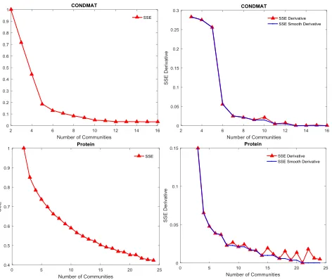
Fig. 6. Variation of SSE(14), derivative of SSE (δk)(15)and smooth derivative (̂_δ

k)(16)withkfor Cond Mat Col and Protein networks (see Table 1).

gradient, each node will converge towards a region of higher density. In this region the density gradient will approach zero because the density will be the same in all directions. Therefore,

consideringpto be the current mode estimate, setting▽f(p) =0

we get the new estimate

ˆ

p= ∑n

j=1pjexp((Λ(p−pj)) ⊺

Λ(p−p_j)/2b2w) ∑n

j=1exp((Λ(p−pj))⊺Λ(p−pj)/2b2w)

. (10)

We repeatedly apply (10) to each node in the network resulting in a drift of each node in each iteration. As a result, nodes follow specific paths in the geodesic space. The final position of a node and its direction of movement are important clue for the

community memberships. Iterations last until the`1norm distance

between the new and the old estimateset+1= ∑nj=1∣∣̂pt+j 1− ̂pj

t_∣∣ 1

is less than a threshold showing that change in position of all nodes is insignificant.

3.3 Estimating Maximum Density Regions

As a node is drifted in the direction of positive density gradient, after a few iterations it will stop because density gradients will become very small in a region of local density maximum. We name the path followed by a node from its starting position to the

stopping position as the node trajectory and the node stopping

position as the trajectory endpoint. Most of the nodes do not

converge to a single point rather stop at different positions in the maximum density region. In order to estimate boundaries of this region, we use a simple algorithm. We randomly pick a trajectory and find its nearest neighbor such that the distance between the two trajectories is minimum at the endpoints (node stopping positions). We simultaneously extend both trajectories as straight lines such that the perpendicular distance between them is minimized. The two nodes may not actually collide rather may pass close to

each other. We compute the corresponding nearest pointsfor all

trajectory pairs and apply linear clustering on the nearest points

and consider each cluster to span a region of maximum density. All

Fig. 7. Variation of SSE(14), derivative of SSE (δk)(15)and smooth derivative (̂_δ

k)(16)withkfor Yeast and Polblogs networks (see Table 1).

nodes converging towards a maximum density region are assigned the same community label.

Consider two trajectories with{p_B,q_B}∈Rnas the trajectory

endpoints. Let{pA,qA}∈R

n

be the points before the end points. Assuming in each of the following iteration, both nodes will keep on moving along the same straight lines with equal drift.

In parametric form a point on each of these straight lines aftert

iterations is

pt=pB+t(pB−pA), (11) qt=qB+t(qB−qA). (12)

Distance between the two lines aftertiterations isdt=pt−qt=

∆B−t(∆B−∆A)where∆A=pA−qA,∆B=pB−qB. Taking

the derivative of squared distance function∂(d⊺

tdt)/∂t=0we get

the value oftofor which error function is minimum:

to=

∆⊺

B(∆B−∆A) ∣∣∆B−∆A∣∣2₂

. (13)

Substituting value of to in (11) and (12) the values of nearest

points{po,qo}is computed. If the two trajectory end points are

very close to each other, then∆B≈0resulting into=0meaning

the trajectory end points are the nearest points.

3.4 Estimating the Number of Communities

K-means clustering is used as a post processing step to divide

the nearest points (defined in the Subsection 3.3) to k clusters.

In many real world networks the division of nearest points into

well-defined groups is challenging, especially whenkis unknown.

Note that other clustering algorithms such as DBSCAN [13] and OPTICS [2] can also be used at this step. However none of the clustering algorithm is parameter free. K-means requires the number of clusters to be input by the user, DBSCAN and OPTICS

both need maximum distance () and minimum number of points

7

K-means objective function is Sum of Squared Error (SSE).

SSE forkclusters given by

k= k ∑ j=1∑i

(pji−cj) ⊺

(pji−cj), (14)

wherepjiis a data point having nearest cluster centercj, therefore

considered member ofj-th cluster. In general, askis increased,

k will decrease and eventually becomes zero when the number

of clusters equals the number of data points. Figures 6 & 7 show

the variation of SSE withkfor four networks. In these networks,

there is no clear indication on the plots when the clustering must be stopped.

Discrete derivative of the objective function (14) w.r.t. k is

given by

δk=

k−k+δk

δk , (15)

whereδk is SSE derivative. We empirically observed that SSE

derivative rapidly decreases from k = 2 to a larger value, then

it becomes a bit transient ask approaches the actual number of

clusters in the network. This behavior of SSE derivative is shown in Figures 6 & 7 for four networks.

We propose a simple smoothing function for the SSE

deriva-tive such that it becomes monotonic decreasing function ofk. If

the current value ofδk>0is larger than a previously seen value

ofδk−p >0, wherep>0 is a positive number, then replace the

current value with the previously seen minimum value.

̂

δk+1=⎧⎪⎪⎨⎪⎪ ⎩

∣δk+1∣ If∣δk+1∣ ≤ ̂δk ̂

δk Otherwise

, (16)

wherêδk+1 is smooth SSE derivative. The required number of

clustersk∗

corresponds tokbeyond whicĥδk≤th, wherethis

a small positive threshold. In networks with not a good clustering

structure, ̂δk may not approach the th. In those cases if ̂δk

remains unchanged for a particular number of clusters. We assume that the appropriate number of clusters has already been achieved

when the minimum value of̂δk+1was obtained.

In Figure 6, for the case of the Protein network, reduction of SSE smooth derivative beyond 21 communities is negligibly small

̂

δ21≤ ̂δ3/100, therefore algorithm selectedk∗=21. In Figure 7,

for the case of Yeast network,̂δ20≤ ̂δ3/40however fork>20,

smooth derivative remains the same for the next four values of

k = {21,22,23,24}. Therefore, algorithm selectedk∗

=20for the Yeast network.

3.5 Complexity Analysis of the Proposed Algorithm

The proposed algorithm has three main steps: computation of geodesic distances, drifting each node towards a local density maximum, and finally the use of k-means community label as-signment. Complexity of each step has been analyzed separately.

The presence of very fast algorithms for computation of shortest paths between all pairs of nodes in a network motivates our choice of using geodesic distances for mapping a network to a geometric space. Pettie and Ramachandran [43] have proposed an algorithm for the all-pairs geodesic distance problem having

the time complexity of O(mnlogα(m, n)), where α(m, n)is

a very slowly growing inverse-Ackermann function, m is the

number of edges, and n is the number of vertices. Recently

Jiang et al. [25] has proposed Quantum Bosonic Shortest Path Searching (QBSPS). For the all-pairs shortest-path problem in

a random scale-free network with n vertices, QBSPS runs in

O(µ(n)ln lnn)time [25].

A simple implementation of the algorithm used in step 2 of

the proposed approach has time complexity ofO(dtn2)whered

is the dimensionality of the space,t is the number of iterations

and n is the nodes in the network. We observe that algorithm

converges quickly, mostly in less than five iterationst≤5. More

efficient implementations of this step are possible by using bucket data structure [27].

Number of iterations may be reduced by using a simple heuristic that if a node comes within a small distance of another node then both will end up in the same final position. Therefore, a previously computed result may be reused. Complexity may

further be reduced by using the locality constraint. If a nodeni

has a final positionpˆi, then all nodes which are initially within a

small distance ofniwill also end up very close topˆi. Therefore,

these nodes may be assigned the same community label asni.

For scalability of the algorithm to larger networks, the di-mensionality of the space has to be reduced by using appropriate dimensionality reduction techniques. We performed some experi-ments using PCA as the dimensionality reduction technique (see Section 4.6). In addition to all these speedup techniques, a parallel implementation of the algorithm can also significantly reduce the execution time.

Computing PCA is equivalent to computing SVD of a

ma-trix. Exact SVD of an m× n matrix has time complexity

O(min{mn2, m2n}). In case of geodesic distance matrix of size

n×n, time complexity of SVD isO(n3). It is one-time cost in

the proposed algorithm and may be performed offline. Therefore, it is feasible for networks with couple of thousands of nodes. For larger networks with millions of nodes, randomized algorithms may be used. Halko et al. [24] have used a randomized version of the block Lanczos method for computing SVD of large matrices

having time complexity O(ikNa+i2k2n), where i ≤ 2, k is

the number of principal components to be computed, Na is the

number of non-zero entries in the matrix.

The third step of the algorithm is post processing of the results generated by step 2. We apply k-means repeatedly with increasing number of clusters until cluster error rate becomes less than a

threshold. If there are k communities in the network, then

k-means will be applied less than k times. Starting with a better

initial estimate will reduce the number of iterations. The running time of Lloyds k-means algorithm, that we used in this work has

time complexity of O(nkdt), wheren is the number of nodes,

k the number of clusters,tthe number of iterations needed until

convergence, anddis the dimensionality of the space.

Thus the dominating factor of time complexity of the proposed

algorithm is O(dtn2) in step 2 of the algorithm. The space

complexity of the proposed algorithm isO(dn)because we have

to storenvectors each of dimensionalityd.

4

E

R

Proposed algorithm is named as Geodesic Density Gradient

(GDG) algorithm for community detection. For all experiments

the values ofα=1/2andβ=1/(n−2)are used in (3) wheren

is the number of nodes in the network. This is because the indirect

distance has(n−2)dimensions and the direct distance has only

two dimensions. These values ofαandβ ensure both distances

become normalized over the number of dimensions. The value

0 0.1 0.2 0.3 0.4 0.5 0.6 0.7 0.8 0.9 1

Mu=7/16

Mu=7.5/16

Mu=8/16

Fig. 8. Normalized Mutual Information (NMI) obtained by different al-gorithms averaged over 100 realizations of GN benchmark network for each value of Mixing Parameterµ= {7/16,7.5/16,8/16}, where 16 is the total degree of each node. The proposedGeodesic Density Gradient (GDG)algorithm has obtained cumulative 35.36% more accuracy than SSCF which is the existing best performing algorithm.

0.43

0.12 0.08 0.12

0.47

0.33

0.18 0.29

0.5 0.59

0.49 0.67

0.79

0 0.1 0.2 0.3 0.4 0.5 0.6 0.7 0.8

Fig. 9. Overall Average Normalized Mutual Information (NMI) obtained by different algorithms over 300 realizations of GN benchmark network. The proposed SGA algorithm has obtained on the average 11.78% more accuracy than SSCF, the existing best performing algorithm.

effect. For the above mentioned values ofα=1/2, β=1/(n−2),

bw=1yielded the best performance.

The GDG algorithm is compared with the existing state of the art methods on two standard benchmark networks with known communities. The performance is compared with 12 existing algorithms including fast modularity optimization by Blondel et al. [4], Markov Cluster algorithm (MCL) [48], Infomap [47], Cfinder [42], fast greedy modularity optimization by Clauset et al.[8], Radicchi et al. [45], algorithm of Girvan and New-man (GN) [18], [38], spectral algorithm by Donetti and Munoz (DM) [12], Expectation-Maximization (EM) algorithm by New-man and Leicht (EM) [40] and Potts model approach by Ronhovde and Nussinov (RN) [46]. In addition to these algorithms compar-isons are also performed with two recent algorithms including Geodesic Sparse Subspace Communities (GSSC) and Sparse Sub-space Communities with Fusion (SSCF) [35]. Experiments are also performed on ten real-world networks.

4.1 Comparisons on GN Benchmark Network

The Girvan-Newman (GN) benchmark [18] has regularly been used to compare the performance of different community detection

algorithms [10], [28]. The network has 128 nodes and four planted ground truth (GT) communities of equal size. Each node has

probability pin of being connected to the nodes of the same

community and pout of being connected to the nodes of the

outside communities. Since the degree of a node is fixed to 16, therefore only one of these two parameters is independent. A

mixing parameterµis defined as the ratio of the external degree

of a node to the total degree. For example,µ=7/16means for

each node out of 16 links, 7 links are to the outside world. For

small values ofµthe structure is well-defined, while forµ≥0.50,

pout≥pin, the graph becomes random with subtle structure.

Experiments are performed by varying the mixing parameter

µ = {7/16, 7.5/16, 8/16}. In each setting, 100 realizations of

the benchmark are used to find an average Normalized Mutual Information (NMI) [10], [30] between the ground truth and the obtained communities. The proposed algorithm has obtained an

NMI={0.997±0.0721, 0.938±0.0758, 0.443±0.0820}respectively.

The NMI comparison is shown in Figures 8 & 9. For all

values ofµ < 7/16the proposed GDG algorithm was obtained

NMI≈1.00, showing 100% accuracy. Forµ =7/16we obtained

average NMI of 99.66% which is higher than all other

algo-rithms under consideration. Forµ =8/16, performance of most

algorithms significantly decreased however the proposed GDG algorithm was able to achieve average NMI of 93.83% which is again significantly larger than all other algorithms.

On this benchmark, on the average, SSCF algorithm of Mah-mmod and Small has remained the second best and the spectral clustering algorithm of Donetti and Munoz (DM) [12] is the third best algorithm. DM was able to obtain good accuracy by using angular distance and complete linkage clustering (see Figure 3 in [12]). Also the number of nodes in this network are only 128 and degree of each node is very high. Due to the small world

effect, maximum geodesic distance in typical GN networks is≤3.

Despite these challenges, the GDG algorithm has performed better than the rest of the existing algorithms including subspace based community detection with fusion (SSCF).

We use T-test to evaluate the statistical significance of the hypothesis that the proposed GDG algorithm is on the average more accurate than the closest competitor SSCF algorithm on GN benchmark. Because the sample is 100 random networks in each of the three settings, degree of freedom is 99 and the

computed value of t is {3.564,9.473,9.360} respectively for

µ = {0.60,0.65,0.70}. Using our results, the hypothesis is

statistically significant for p-value≤0.05%for all settings.

4.2 Comparisons on the LFR Benchmark

The Lancichinetti-Fortunato-Radicchi (LFR) benchmark [31] has power law degree distribution and community sizes are also variable, presenting more challenges to the community detec-tion algorithms. In this experiment, the number of nodes in the network is 1000, the average degree is 20 and the maximum degree is 50. Minimum ground truth community size is 30 and maximum is 100. Therefore, the number of ground truth communities may vary from 10 to 33. The mixing parameter is

variedµ= {0.60,0.65,0.70}. For each setting, 100 networks are

randomly generated by using the implementation of the original authors [28]. The detected communities are compared with the ground truth by using NMI [30]. The proposed algorithm has

achieved NMI={0.834±0.0710, 0.600±0.0759, 0.240±0.0662}

9

0 0.1 0.2 0.3 0.4 0.5 0.6 0.7 0.8 0.9 1

Mu=0.60 Mu=0.65 Mu=0.70

0.7

Fig. 10. Normalized Mutual Information (NMI) obtained by different algorithms averaged over 100 realizations of LFR benchmark network for each value of the Mixing Parameterµ= {0.60,0.65,0.70}. Overall accuracy improvement of the proposed GDG algorithm is 13.73% over the existing best performing algorithm SSCF of Mahmood and Small.

0.41

0.01 0.09

0.37

0.09 0.04

0.01 0.07

0.25

0.01 0.33

0.42 0.51

0.56

0 0.1 0.2 0.3 0.4 0.5 0.6 0.7

Fig. 11. Average Normalized Mutual Information (NMI) obtained by different algorithms over 300 realizations of LFR benchmark network. Average accuracy improvement of the proposed GDG algorithm is 8.10% over the existing best performing algorithm SSCF of Mahmood and Small.

algorithm, results are reported for the random initialization. Due to variable degree, communities of different sizes and increased mixing parameter, the performance of all algorithms has reduced compared to GN benchmark. An NMI comparison for different algorithms is shown in Figures 10 and 11.

The performance of subspace based community detection GSSC algorithm has improved on this benchmark and it has become the second best algorithm. It is because of increased num-ber of nodes and comparatively lower average node degree. The performance of DM [12] algorithm has significantly deteriorated due to more challenges. Other algorithms including Blondal et al.,

infomap and RN performed better forµ=0.60while forµ=0.65

only the algorithm of Blondal et al. has shown comparatively

good performance. For µ = 0.70 all existing algorithms except

GSSC and SSCF have shown almost zero performance. It is because the modularity based methods perform poor when the community size reduces and the network size increases [15]. Also for zero or negative detectability thresholds, the performance of these methods deteriorate. The proposed GDG algorithm has

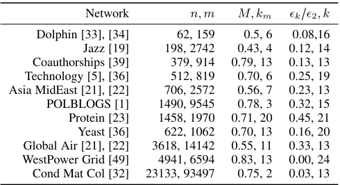
TABLE 1

Results of the proposed GDG algorithm on 11 real-world networks,

n, mare the number of nodes and edges,M, kmare the maximum modularity and corresponding number of communities,k/2, kare the

normalized clustering error and corresponding communities.

Network n, m M, km k/2, k

Dolphin [33], [34] 62, 159 0.5, 6 0.08,16 Jazz [19] 198, 2742 0.43, 4 0.12, 14 Coauthorships [39] 379, 914 0.79, 13 0.13, 13 Technology [5], [36] 512, 819 0.70, 6 0.25, 19 Asia MidEast [21], [22] 706, 2572 0.56, 7 0.23, 13 POLBLOGS [1] 1490, 9545 0.78, 3 0.32, 15 Protein [23] 1458, 1970 0.71, 20 0.45, 21 Yeast [36] 622, 1062 0.70, 13 0.16, 20 Global Air [21], [22] 3618, 14142 0.55, 11 0.33, 13 WestPower Grid [49] 4941, 6594 0.83, 13 0.00, 24 Cond Mat Col [32] 23133, 93497 0.75, 2 0.03, 13

obtained 24.03% NMI for µ = 0.70 which is an improvement

over the current best method. More accuracy of GDG algorithm

for µ = {0.65,0.70} shows the capability of the approach to

accurately detect communities in more challenging situations. We use T-test to evaluate the statistical significance of the hy-pothesis that the proposed GDG algorithm is on the average more accurate than the closest competitor SSCF on LRF benchmark. Because the sample is aganin 100 networks therefore DOF is 99

and we foundt= {2.256,8.721,2.89}respectively for the three

settings. Using our results, the hypothesis is statistically significant

for p-value≤{2.5 %, 0.05 %, 0.5%}respectively.

4.3 Experiments on Real-World Networks

In real-world networks, there is no ground truth node labeling therefore it becomes difficult to compare the accuracy of the proposed algorithms with the existing methods. Also most of the existing methods try to maximize modularity which has recently been found to not be capable of resolving communities of smaller

sizes. Therefore we report both the modularityM and the

cluster-ing errorkcorresponding to minimum error derivative (Table 1).

For each network, we normalize the k-means clustering error over

two clusters (2) to 1.00 and scale the error overk>2clusters as

k/2. Results are reported for GDG algorithm with fixed value of

bw=1/ √

2.

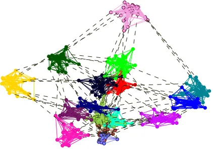
Experiments are performed on eleven real world networks and the results are summarized in Table 1. Number of nodes in these networks vary from 62 to 23133. For each network we compare the communities found by maximum modularity with those found by the proposed algorithm. The structure of the five of these networks is shown in the geodesic space along with communities in Figure 12.

In the networks with well-defined community structure, the

k/2 is significantly smaller than 1.00. For example consider

10 -2 5 0 -2 0 0 -1 5 0 -1 0 0 -5 0 0 50 -4

0 -20 0 20 40

-4 0 0 -2 0 0 -3 0 -2 0 -1 0 0 10 20 30 40 50

0 0 0 0

-2

5

0 -20₀ -1₅ 0 -10₀ -5

0 -6 0 -4 0 -2 0 0 20 40

60 -30 -20 -10 0 10 20 30

(a) (b) (c) (d) (e)

Fig. 12. (a) A two level hierarchical structure of the Jazz Bands network. The two main partitions correspond to bands in the New York and Chicago and further division shows the segmentation of black and white bands in each partition. (b) Largest connected component of Coauthorship network consisting of 13 communities. (c) Electronic circuits network. (d) Transcription Yeast network. (e) POLBLOGS network showing two main groups in 2004 US election. Tracks of node movements are also shown.

(a)

(b)

Fig. 13. Western Power Network has exhibited very strong community structure with almost zero residual error for 24 clusters (b). Trajectory end points after convergence.

can be viewed in Figure 13a. For this network, for 24 communities

shown by different colors in Figures 13a and 13b,24/2<.005.

The Condensed Matter network (COND-MAT) [32] with 23,133 nodes and 93,497 edges also has a well-defined community structure (see Table 1). This network covers scientific collabo-rations between authors of papers submitted to the Condensed Matter category in arXiv. The nodes indicate authors and the links indicate co-authorship’s. For this network in our algorithm

13/2 < 0.03 indicates that network has 13 compact

commu-nities. Maximum modularity of 0.75 was obtained for only two communities. Thus for this network, modularity maximization has completely failed to capture the network structure because network definitely have large number of communities.

The Technology Graphs [5], [36] are constructed from elec-trical circuits, where nodes represent logic gates and flip-flops. The 6 communities shown in Figure 12c correspond to maximum modularity of 0.70. In the geodesic space, this network has a conical structure which is open from one side. All nodes close to the apex of the cone are in one community, the surface of the cone is divided into five communities and protruding nodes have formed the 6-th community. The number of communities corresponding to minimum smooth error given by (16) is 19 and

the corresponding19/2<0.25, which shows that this network

-50 -40 -30 -20 -10 -20 -10 0 10 20 -6 -4 -2 0 2 4 6 -50 -40 -30 -20 -10 -20 -10 0 10 20 -6 -4 -2 0 2 4 6 -50 -40 -30 -20 -10 -20 -10 0 10 20 -6 -4 -2 0 2 4 6 -50 -40 -30 -20 -10 -20 -10 0 10 20 -6 -4 -2 0 2 4 6 -50 -40 -30 -20 -10 -20 -10 0 10 20 -6 -4 -2 0 2 4 6 -50 -40 -30 -20 -10 -20 -10 0 10 20 -6 -4 -2 0 2 4

6 (a) (b) (c)

(d) (e) (f)

Fig. 14. GDG Algorithm: (a)-(f) hierarchical structure of the Dolphins network is revealed by increasing clusters from two to seven. Each time clustering is independently performed but the cluster boundaries are mostly preserved, demonstrating stability of the communities.

has a weak community structure.

4.4 Hierarchical Structure

The proposed GDG algorithm can also reveal hierarchical struc-ture of a network, if such strucstruc-ture exists. For example, hier-archical structure of the Dolphin social network [33], [34] is revealed when the number of communities is increased from 2 to 7 (Figure 14). Similarly, two level hierarchical structure of Jazz Bands Network [19] is shown in Figure 12a.

Zachary Karate Club [50] is one of the commonly used network for community detection experiments. This network rep-resents friendships between the 34 members of a karate club and

has 77 links. By increasing the number of communities (K) from

2 to 6 we observe a hierarchical structure in this network (Figure

15). ForK = 2the two detected communities are marked as L

andRin Figure 15. These communities are exactly the same as

the club later broke down. We observe split of a small community

{3, 9, 14, 21} in Figure 15 such that {3, 14, 20} are part of

the administrator group (with node 1) and{9}is the part of the

instructor group (with node 33). As the number of communities is

increased to 3,Lsplit intoL1andL2whileRremained intact.

However withK=4,Ralso split intoR1andR2communities.

This reveals a perfect hierarchical structure in this network. For

11

Fig. 15. Hierarchical structure of Karate club network is marked with different ellipses. Two first level communities are L and R. Four second level communities are L1, L2, R1, R2 and four third level communities are L1a, L1b, R1a, R1b.

We observe L1a to be a disconnected community however the

nodes {9, 10, 28, 29, 31, 32} are globally close. There are no

direct links between three groups{28, 29, 32},{9, 31}and{10}.

The global similarity can be visually observed from Figure 15

where all nodes inL1aare closer to theRwhile the nodes inL1b

are relatively distant fromR. A further increaseK=6caused a

split ofR1toR1aandR1b. The three nodes ofR1{3, 14, 20}

are close to the boundary of L andR communities. The nodes

{3,14}split from rest of the nodes and formed a new community

R1bwhich makes the third level of hierarchy.

These experiments demonstrate the capability of the proposed GDG algorithm to detect hierarchical communities. Note that the hierarchical structure is not imposed rather only the number of communities are varied and communities are independently found each time.

4.5 Consistency of Community Occupancy

We also performed consistency of community-occupancy analysis by varying the number of communities and computing the

occu-pancy map each time. The occuoccu-pancy map Mo has size n×n

andMo(i, j) =1if a pair of nodesi, jis in the same community,

otherwiseMo(i, j) =0. Integration of all occupancy maps yielded

an overall map showing the pairs which were for a given number of times in the same community. For the Karate Club network

we varied the number of communities asK= {2,3,4,5,6}. The

integrated occupancy map and histogram of node pairs based on consistency is shown in Figure 16. In this network we observe 19.55% of the pairs remained 100% consistent while 52.768% pairs never existed. Due to hierarchical community structure, as the communities are increased from 2 to 6, the occupancy pattern changes significantly. Based on consistency, we can classify the node pairs being never in the same community, or a given number of times in the same community. Such a classification of nodes pairs is shown in Figure 16a, in which each class is shown by a different color. The color to consistency mapping is shown in the histogram where color of a bar encodes the consistency value and length of the bar represents the probability of the node pairs of a particular consistency. By using this analysis we identify the core

(a) (b)

5 10 15 20 25 30

0 5 10 15 20 25 30 35 0 0.1 0.2 0.3 0.4 0.5

0 1 2 3 4 5

P

ro

b

a

b

ili

ty

o

f

N

o

d

e

P

a

ir

s

Consistency of Occupancy

Fig. 16. (a) Integrated consistency map of Karate Club network forK= {2,3,4,5,6}andbw=1.0. (b) Consistency histogram.

200 250 300 350 400 450 500 550 600 650 700 Increasing Dimensionality in steps of 20

0 0.1 0.2 0.3 0.4 0.5 0.6 0.7 0.8

Normalized Mutual Information

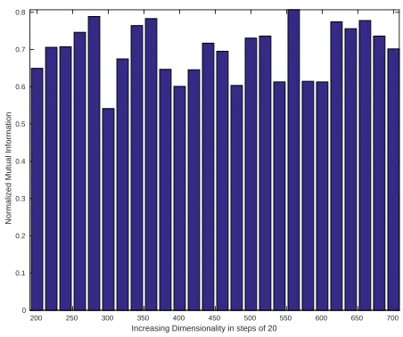
Fig. 17. NMI between the original communities and the low dimensional communities in the Asia MidEast network, starting from 200 dimensional subspace.

of each community which are most consistent set of nodes in that community.

4.6 Scalability of the Proposed Algorithm to Bigger Networks

As the number of nodes in a network increases, the dimensionality of the corresponding geodesic space will also increase. In very high dimensional spaces, the performance of clustering algorithms may degrade. To make the proposed algorithm applicable to bigger networks, dimensionality reduction needs to be performed over the geodesic space. In this section, we consider PCA for dimensionality reduction. We find the principal components of the

geodesic space and project all geodesic vectors onp<nprincipal

dimensions. As a result, we get p dimensional geodesic space.

We apply the proposed algorithm in this space. Comparison of the communities found in low-dimensional space with the original communities reveals a good match in most cases, as discussed below.

5 10 15 20 25

Increasing Dimensionality in Multiples of 20

5

10

15

20

25

Increasing Dimensionality in Multiples of 20

0.5 0.55 0.6 0.65 0.7 0.75 0.8 0.85 0.9 0.95 1

Fig. 18. NMI across low dimensional communities in the Asia MidEast network shown as heat-map. Starting dimensionality shown as 1 is 200 dimensional space. Each increment is of 20 dimensions in the order of reducing eigenvalues.

100 200 300 400 500 600

Increasing Dimensionality in steps of 20 0

0.1 0.2 0.3 0.4 0.5 0.6 0.7 0.8 0.9

Normalized Mutual Information

Fig. 19. NMI between the original communities and the low dimensional communities in the Yeast network, starting from a 20 dimensional sub-space. NMI increases with the increasing dimensionality from 20 to 300 dimensions. Beyond that NMI remains almost the same.

proposed algorithm by varying the dimensionality of the space. We used Normalized Mutual Information (NMI) to find the similarity between the communities found in reduced dimensionality spaces and the original communities. The Asia MidEast network has 706 nodes. See details of the network in Table 1. By using the proposed DGD algorithm, 13 communities were found corresponding to the minimum clustering error gradient. We projected the network to

{200,220,⋯,700} dimensional spaces and independently

iden-tified 13 communities in each subspace. Then NMI is computed between the communities in each subspace and the original com-munities, as shown in Figure 17. In this experiment, the average

NMI is0.70±0.072. Communities found for the low-dimensional

sub-spaces are also compared with each other and the resulting NMI has been shown as a heat map in Figure 18. The overall

average NMI is0.721±0.1043.

Similar experiments have also been performed for the Yeast network having 662 nodes. See details of the Yeast network in Table 1. We varied the dimensionality of the geodesic space

5 10 15 20 25 30

Increasing Dimensionality in Multiples of 20

5

10

15

20

25

30

Increasing Dimensionality in Multiples of 20

0.2 0.3 0.4 0.5 0.6 0.7 0.8 0.9 1

Fig. 20. NMI across low dimensional communities in the Yeast network shown as heat-map. The second row and 2nd column are the starting dimensionality which is 20 dimensional space. Each increment is of 20 dimensions in the order of reducing eigenvalues. First column and first row show the NMI between each lower dimensional community with the full dimensionality communities.

as follows {20,40,⋯,660}. For each dimensionality, network

is divided into 21 communities. NMI computed between the communities found in low-dimensional subspace and the original communities is shown in Figure 19. The average NMI is found

to be 0.7508±0.158. We observe a higher NMI for subspaces

with dimensionality 200 or more. In this case, average NMI is 0.7915+0.0452. NMI found between low dimensional commu-nities is shown as a 2D heat map in Figure 20. In this

exper-iment, overall average NMI is 0.6731±0.1843. NMI between

communities in 200 dimensional sub-spaces or higher has average

0.7813±0.100. The first column and first row in this map is the

NMI of each low dimensional set of communities with the original communities.

These experiments demonstrate that a dimensionality reduc-tion technique preserving distances between the points as in the original space will result in higher similarity between the communities in the low dimensional space and the communities in the original space.

4.7 Execution Time Comparisons

Execution time of the proposed GDG algorithm has been com-pared with two recent algorithms GSSC and SSCF [35] for six different networks on Intel 2.7GHz quad-core i5 processor machine with 16GB RAM as shown in Figure 21. For smaller networks such as Karate and Football the three algorithms are quite fast. For the synthetic LFR network having 1000 nodes, the execution time of both GSSC and SSCF increases with the

increasing value of the mixing parameterµ. However the proposed

GDG algorithm is not much effected due to increased network complexity. For the case of polblog network having 1490 nodes the proposed GDG algorithm has performed much faster than the subspace based algorithms. It is because the performance of subspace based algorithms is dependent on the the network complexity while the proposed algorithm is not much effected.

5

C

13

0 5 10 15 20 25

Karate Football Polblog LFR_0.6 LFR_0.65 LFR_0.70

E

X

E

C

U

T

IO

N

T

IM

E

I

N

S

E

C

O

N

D

S

GDG GSSC SSCF

Fig. 21. Execution time of the proposed GDG algorithm compared with two recent algorithms GSSC and SSCF [35] on three real networks (Karate (nodes=34, edges=78), Football(nodes=115, edges=631), Pol-blog(nodes=1490, edges=16716)) and three synthetic networks (LFR

µ= {0.60,0.65,0.70}(nodes=1000, edges=9774)). The proposed GDG algorithm is faster than both of these current algorithms.

absence of a link between two entities is known. For recognition of structural patterns in these systems, the network nodes need to be mapped to a geometric space. In this paper we proposed using

geodesic distance vectors for this purpose. A Geodesic Density

Gradient (GDG)algorithm is proposed to find communities and to reduce the error at the community boundaries.

The proposed GDG algorithm is based on a distance mea-sure specifically designed for improved community detection in geodesic space. Each node in the geodesic space is shifted towards a positive density gradient until convergence is obtained overall nodes. In a post processing step, the number of communities is

increased from a minimum value (k ≥ 2) to a larger number

and the variation of the clustering error derivative is observed. Initially the error derivative decreases rapidly and then it slows down and after a particular number of communities the error derivative becomes less than a threshold yielding the number of communities.

The variation of the number of communities gave an oppor-tunity to study hierarchical community structure. As the num-ber of communities is increased, coarser communities split into finer ones revealing a hierarchical community structure in the network. Splitting of coarser communities is not forced rather the optimization is independently applied for increased number of communities. A perfect hierarchical structure was observed in some real world networks such as Karate club network and the Dolphin social network.

Consistency of community occupancy is also studied by vary-ing the number of communities and countvary-ing the co-occupancy of each pair of nodes. Node pairs having very high consistency form the core of each community. The nodes which are outside the core may switch partitions and therefore may be considered members of more than one community as is the case of overlapped community structure.

The focus of the current work has remained on non-overlapped community detection by considering a node to be member of only one community at a time. An important future goal of our research is to extend it for overlapped and time varying community detection.

A

This work is funded by an Australian Research Council Discovery Project (DP140100203). M. Small is supported by an Australian

Research Council Future Fellowship (FT110100896).

R

[1] L. Adamic and N. Glance. The political blogosphere and the 2004 US election: divided they blog.Proc. 3rd Int. Workshop on Link Discovery, 411:36–43, 2005.

[2] M. Ankerst, M. M. Breunig, H.-P. Kriegel, and J. Sander. Optics: ordering points to identify the clustering structure. In ACM Sigmod Record, volume 28, pages 49–60. ACM, 1999.

[3] A. L. Barabasi.Network Science (online available: barabasilab.neu.edu

/ networksciencebook). 2012.

[4] V. D. Blondel, J.-L. Guillaume, R. Lambiotte, and E. Lefebvre. Fast unfolding of communities in large networks j.Stat. Mech.: Theory Exp., page P10008, 2008.

[5] R. F. Cancho, C. Janssen, and R. V. Sole. Topology of technology graphs: Small world patterns in electronic circuits. Phys. Rev. E, 64:046119, 2001.

[6] J. Chen and Y. Saad. Dense subgraph extraction with application to community detection.IEEE TKDE, 24(7):1216–1230, July 2012. [7] Y. Cheng. Mean shift, mode seeking, and clustering. Pattern Analysis

and Machine Intelligence, IEEE Transactions on, 17(8):790–799, 1995.

[8] A. Clauset, M. E. J. Newman, and C. Moore. Finding community structure in very large networks.Phys Rev. E, 70:066111, 2004. [9] D. Comaniciu and P. Meer. Mean shift: A robust approach toward

feature space analysis.Pattern Analysis and Machine Intelligence, IEEE

Transactions on, 24(5):603–619, 2002.

[10] L. Danon, A. Daz-Guilera, and A. Arenas. The effect of size heterogene-ity on communheterogene-ity identification in complex networks j.Stat, 2006. [11] D. Deritei, Z. I. L´az´ar, I. Papp, F. J´arai-Szab´o, R. Sumi, L. Varga, E. R.

Regan, and M. Ercsey-Ravasz. Community detection by graph voronoi diagrams.New Journal of Physics, 16(6):063007, 2014.

[12] L. Donetti and M. A. Munoz. Detecting network communities: a new systematic and efficient algorithm. Journal of Statistical Mechanics:

Theory and Experiment, 2004(10):P10012, 2004.

[13] M. Ester, H.-P. Kriegel, J. Sander, and X. Xu. A density-based algorithm for discovering clusters in large spatial databases with noise. InKdd, volume 96, pages 226–231, 1996.

[14] S. Fortunato. Community detection in graphs. Physics Reports, 486(3):75–174, 2010.

[15] S. Fortunato and M. Barthlemy. Resolution limit in community detection.

Proc. Natl. Acad. Sci. USA, 104:36–41, 2007.

[16] M. V. Fragkiskos D. Malliaros. Clustering and community detection in directed networks: A survey.Physics Reports, 533(4):95–142, 2013. [17] M. Girvan and M. E. Newman. Community structure in social and

biological networks. Proceedings of the National Academy of Sciences, 99(12):7821–7826, 2002.

[18] M. Girvan and M. E. J. Newman. Community structure in social and biological networks. Proceedings of the National Academy of Sciences, 99(12):7821–7826, 2002.

[19] P. M. Gleiser and L. Danon. Community structure in jazz. Advances in

complex systems, 6(04):565–573, 2003.

[20] M. Gong, J. Liu, L. Ma, Q. Cai, and L. Jiao. Novel heuristic density-based method for community detection in networks. Physica A: Statistical

Mechanics and its Applications, 403:71–84, 2014.

[21] R. . Guimer, M. Sales-Pardo, and L. A. N. Amaral. Classes of complex networks defined by role-to-role connectivity profiles. Nature Physics, 3:63–61, 2007.

[22] R. Guimer, S. Mossa, A. Turtschi, and L. A. N. Amaral. The worldwide air transportation network: Anomalous centrality, community structure, and cities’ global roles. Proceedings of the National Academy of

Sciences, 102(22):7794–7799, 2005.

[23] J. H, M. S, B. A. L, and O. Z. N. Lethality and centrality in protein networks.Nature, 411, 2001.

[24] N. Halko, P.-G. Martinsson, Y. Shkolnisky, and M. Tygert. An algorithm for the principal component analysis of large data sets. SIAM J. Sci.

Comput., 33(5):2580–2594, Oct 2011.

[25] X. Jiang, H. Wang, S. Tang, L. Ma, Z. Zhang, and Z. Zheng. A new approach to shortest paths on networks based on the quantum bosonic mechanism.New Journal of Physics, 13:013022, 2013.

[26] H. Jin, S. Wang, and C. Li. Community detection in complex networks by density-based clustering. Physica A: Statistical Mechanics and its

Applications, 392(19):4606–4618, 2013.

[27] J. N. Kaftan, A. A. Bell, and T. Aach. Mean Shift Segmentation Evaluation of Optimization Techniques. In Proceedings of the Third International Conference on Computer Vision Theory and Applications,

VISAPP 2008, pages 365–374, Funchal, Madeira - Portugal, January