Suspiciously Timed Trade Disputes
∗
Paola Conconi
1,2, David R. DeRemer
3, Georg Kirchsteiger
1,2,4,5,
Lorenzo Trimarchi
1, and Maurizio Zanardi
61ECARES, Universit´e Libre de Bruxelles
2CEPR 3Institute of Economics, Hungarian Academy of Sciences
4CESifo 5VCEE6Lancaster University Management School
June 2016
Abstract
This paper shows that electoral incentives crucially affect the initiation of trade dis-putes. Focusing on WTO disputes filed by the United States during the 1995-2014 period, we find that U.S. presidents are more likely to initiate a dispute in the year preceding their re-election. Moreover, U.S. trade disputes are more likely to involve industries that are important in swing states. To explain these regularities, we develop a theoretical model in which re-election motives can lead an incumbent politician to file trade disputes to appeal to voters motivated by reciprocity.
JEL classifications: F13, D72, D78, D63.
Keywords: Trade disputes, elections, reciprocity.
∗We are grateful to Chad Bown, Meredith Crowley, Bal´azs Murak¨ozy, David Rietzke, and G´erard Roland
1
Introduction
Media coverage of the 2012 United States presidential election suggests that trade disputes
mattered in the re-election campaign of Barack Obama. An article in the Economist noted a “suspiciously timed dispute” filed against China in the World Trade Organization (WTO)
less than two months before Obama’s re-election.1 Not only the timing of the disputes was
suspicious, but also the fact that it involved the automobile industry, a large employer in
Ohio, a crucial “swing state” in the U.S. presidential election:
There was nothing subtle about the American government’s lodging of a trade complaint on September 17th, alleging that China unfairly subsidises car-part exports on the same day that Barack Obama was campaigning in the crucial swing state of Ohio—home to many car-part suppliers. But then subtlety does not win many elections.
Later media coverage observed that Obama “frequently touted a series of cases” against
China which were “occasionally timed to campaign stops in industrial swing states in the
Midwest” (“US in trade dispute with Indonesia,” Financial Times, January 10, 2013). Obama has not been unique among U.S. presidents in filing disputes that figured
promi-nently during a re-election campaign. Less than a month before his re-election date, George
W. Bush filed a dispute at the WTO against the European Union for allegedly subsidizing
Airbus. During the third presidential debate between Bush and John Kerry, Kerry
com-mented: “This president didn’t stand up for Boeing when Airbus was violating international
rules and subsidies. He discovered Boeing during the course of this campaign after I’d
been talking about it for months” (“October 13, 2004 Debate Transcript,” Commission on Presidential Debates).
Our paper provides systematic empirical evidence that electoral incentives affect the
filing of trade disputes. We study WTO disputes initiated by the United States. There
are three main reasons to focus on the U.S. First, it is the country that has filed the most
WTO disputes. Second, the existence of executive term limits creates variation in electoral
incentives both within and across U.S. presidents, who have direct control over the decision
to initiate WTO disputes. Finally, we can observe variation over time in the electoral
importance of different U.S. states and industries.
We construct a database of all WTO disputes initiated by the United States during the 1995-2014 period. To verify whether U.S. trade disputes are “suspiciously timed” close to
the president’s re-election, we collect each dispute’s initiation date. We also match each
dispute to one or more NAICS 3-digit codes. This allows us to study industry determinants
1“Chasing the anti-China vote: A suspiciously timed dispute,”The Economist, September 22, 2012.
of U.S. trade disputes. In particular, we can verify whether U.S. presidents are more likely
to initiate disputes to support important industries in swing states (e.g. the automotive
industry in Ohio). We identify swing states based on the margin of victory in the most
recent presidential election. To capture the importance of an industry in these battleground states, we calculate the percentage share of workers over all swing states that are employed
in the industry. To capture the importance of an industry in these battleground states, we
calculate the industry’s employment summed across swing states over total employment in
swing states. Crucially, these employment shares vary over time, due both to changes in
the identity of the swing states and changes in the employment structure across industries
within states.
A first descriptive look at the U.S. dispute history in Figure 1 already suggests that
re-election motives affect the initiation of trade disputes. Each bar represents the number
of disputes filed by the U.S. in each year between 1995 and 2014.2 The dashed lines show an increase in disputes during the first term of the three presidents, when they could still
be re-elected. There is no clear pattern in the disputes during the second terms, when the
[image:3.612.88.528.415.679.2]presidents faced terms limits and thus had no re-election motive.
Figure 1: WTO disputes filed by the U.S., by year of presidency
Clin ton II I Clin ton IV Clin ton bis I Clin ton bis II Clin ton bis II I Clin ton bis IV GWBush I GWBush II GWBush II I GWBush IV GWBush bis I GWBush bis II GWBush bis II I GWBush bis IV Obama I Obama II Obama II I Obama IV Obama bis I Obama bis II 0 5 10 15 20
Our industry-year panel data analysis of the determinants of U.S. trade disputes provides
2As we detail in Section 2, our definition of year accounts for differences in the electoral, inaugural, and
more systematic evidence of the importance of electoral incentives. Our results confirm that
U.S. presidents are more likely to initiate WTO disputes during the last year of their first
term (re-election year effect). With respect to sectoral composition, we find that U.S. trade
disputes are more likely to involve industries that are important in swing states (swing industry effect). We show that these results are robust to including broad industry fixed
effects, different time fixed effects (President or President-Term), as well as many different
controls accounting for other possible determinants of trade disputes, both at the sectoral
level (e.g. the size of the industry in the U.S. at large, its degree of concentration, and the
growth rate of imports and exports) and aggregate level (e.g. changes in unemployment
and the exchange rate). They also continue to hold when we use alternative econometric
methodologies to study the determinants of trade disputes (linear probability model, probit,
or negative binomial). In terms of magnitude, the estimates of our baseline regressions
indicate that the re-election year effect and the swing industry effect are sizeable. Trade disputes are between 13.5 and 21.7 percentage points more likely to be initiated in
re-election years; and a marginal increase in importance of an industry in swing states raises
the probability that the U.S. initiates a dispute involving that industry by between 18.3 and
30.8 percentage points.
To interpret our empirical findings, we develop a tractable political economy model of
trade disputes. There are three main actors in the model: the incumbent politician, a
challenger, and the median voter. Politicians serve one-period terms and can only be
re-elected once. In the first period, the incumbent decides whether to file a dispute. At the
end of this period, the voter decides whether to elect the incumbent or the challenger. In the second period, the elected politician decides whether to file a dispute, if it was not filed
prior to the election. Politicians are office motivated and, all else equal, prefer not to file the
trade dispute.
They key assumption of our theoretical model is that voters have reciprocal preferences,
i.e. they like to act kindly to politicians who have helped them and unkindly to politicians
who have harmed them. We build on a vast theoretical literature, which emphasizes the
importance of reciprocity and fairness (e.g. Rabin, 1993; Fehr and Schmidt, 1999;
Dufwen-berg and Kirchsteiger, 2004; Falk and Fischbacher, 2006).3 In recent years, experimental
economists have gathered overwhelming evidence that individuals reward kind actions and punish unkind ones (e.g. Fehr, G¨achter, and Kirchsteiger, 1997; Charness and Dufwenberg,
2006; Kube, Mar´echal, and Puppe, 2012). Models of reciprocity have been also been applied
3We focus on intrinsic reciprocity instead of the “instrumental” reciprocity that can result from optimizing
behavior of selfish agents (Sobel, 2005). Models of instrumental reciprocity include vote-buying (e.g. Dekel, Jackson, and Wolinsky, 2008) and clientelism, i.e. the literal exchange of favors or policies for political support (e.g. Kitschelt and Wilkinson, 2007; and Robinson and Verdier, 2013).
to political economy (e.g. Hahn, 2009), and recent influential work by Finan and Schechter
(2012) provides strong empirical and experimental evidence that voters like to help
politi-cians who have been kind to them, and to punish politipoliti-cians who have been unkind to
them.
We first show that, if voters have standard preferences (no reciprocity), they will choose
between the incumbent and the challenger based on their ideological preferences. In this
case, politicians will never file a trade dispute, even if they are office motivated and know
that voters would like a dispute to be filed. This is because, if voters are fully rational, their
decisions are unaffected by whether or not a politician has filed a dispute. We then show
that, if votes have reciprocal preferences, the unique equilibrium involves the incumbent
filing the dispute prior to the election and increasing his chance of re-election, provided
that the voter’s ideological preference for either candidate is sufficiently small relative to the
voter’s preference for the trade dispute. When the voter narrowly prefers the challenger, the incumbent’s ability to file a dispute provides an advantage over the challenger who
cannot commit to file the dispute after the election. The voter’s motivation to reciprocally
reward the incumbent for filing the dispute dominates the voter’s ideological preference for
the challenger, so the voter chooses the incumbent. When the voter narrowly prefers the
incumbent, the incumbent will still file the dispute, because otherwise the voter’s desire
to be unkind to the incumbent would dominate the voter’s ideological preference for the
incumbent.
Our theoretical model provides a simple explanation for our empirical findings concerning
the timing of U.S. trade disputes (the re-election effect) and their composition (the swing industry effect). An alternative rationale for our findings could be provided by a model
in which the incumbent politician initiates disputes to signal his trade policy preferences
to voters. Our model shows that, even if voters have full information about politicians’
preferences, electoral incentives can still shape trade policy outcomes. A full information
model has particular advantages in our empirical context. First, specifying how politicians
signal preferences is much less straightforward for disputes than for conventional trade
pro-tection. While higher import tariffs are clearly a more protectionist policy than lower tariffs,
trade disputes have more diverse implications. In particular, we can observe that the same
president in the same year initiates disputes promoting trade and others aimed at reducing trade.4 Moreover, our model predicts electoral cycles for all politicians, which is consistent
4For example, Obama’s re-election year included two disputes distinctly affecting automotive industry
with our results on the re-election year effects. Signalling models would instead predict
electoral cycles only for particular types of politicians.5
Our paper is related to several streams of literature, beyond the above-mentioned
lit-erature on reciprocity. Recent studies examine the determinants of WTO trade disputes (e.g. Horn, Johannesson, and Mavroidis, 2011; Bown and Reynolds, 2015a, 2015b; Kuenzel,
2014; and Li and Qiu, 2014). Closest to our analysis is the paper by Rosendorff and Smith
(2013), who study the role of power change. Chaudoin (2014) considers electoral cycles for
disputes filed against the U.S. To the best of our knowledge, ours is the first paper to show
that re-election motives affect trade disputes. A recent study by Pervez (2015) provides
cross-country evidence that governments tend to file WTO disputes over antidumping duties
close to elections. Our paper is distinct in that we focus on the United States—in which the
existence of executive term limits creates exogenous variation in electoral incentives—and
show that re-election motives affect the timing and industry composition of all types of trade disputes filed.
Our finding that U.S. trade disputes tend to target industries that are important in
swing states is reminiscent of Muˆuls and Petropoulou (2013). They find that U.S. trade
policy responds to the interests of swing states, based on a cross-section of industries near
the 1984 election and an index of non-tariff trade policies. Similarly, Ma and McLaren (2016)
consider how swing state incentives affect the import tariffs set in trade agreements. Our
paper studies how both swing state incentives and electoral calendars affect the filing of
WTO disputes.
Our analysis is also related to the literature that studies how electoral calendars affect policy choices. Theoretical work by Rogoff (1990) and Rogoff and Sibert (1988) suggests that,
close to elections, incumbent politicians manipulate regular government decisions on fiscal
and monetary policies to signal their competence. Drazen (2001) surveys the macroeconomic
literature on presidential electoral cycles and concludes that there is limited evidence in U.S.
fiscal policy after 1980 and no evidence in U.S. monetary policy.6 Recent studies find evidence
of electoral cycles in executives’ decisions on inter-state conflicts (Conconi, Sahuguet, and
Zanardi, 2014) and in legislators’ voting behavior (Conconi, Facchini, and Zanardi, 2014;
Bouton, Conconi, Pino, and Zanardi, 2014).
5Muˆuls and Petropoulou (2013) consider voters who are uncertain about whether a politician is a “free
trader” or “protectionist” and politicians who also differ in whether their trade policy preferences are weak or strong. Electoral cycles and signals are observed only when incumbent politicians are weak free-traders, who must be in the minority among free traders for the signal to be credible.
6A large literature stresses voters’ resistance to electoral manipulation (e.g. Peltzman, 1992; Shi and
Svensson, 2006; and Brender and Drazen, 2008). Among developed countries, Brender and Drazen (2005) find no evidence of electoral cycles in budget deficits, but Brender and Drazen (2013) do find electoral cycles in broad categories of government expenditure.
The rest of the paper proceeds as follows. Section 2 describes the data. Section 3 details
the empirical strategy and results. Section 4 describes the theoretical model. Section 5
concludes, discussing the broader implications of our analysis for the effectiveness of the
WTO.
2
Dataset and variables
In our empirical analysis, we study the determinants of WTO disputes initiated by the United
States. We choose to focus on WTO disputes, disregarding trade disputes filed under the
General Agreement on Tariffs and Trade (GATT). This is because under the GATT system,
member countries could veto the initiation of a dispute. Moreover, rulings could only be
adopted by consensus, implying that a single objection could block the ruling.7 By contrast, under the dispute settlement procedure established by the WTO, rulings are automatically
adopted unless there is a consensus to reject a ruling: any country wanting to block a ruling
has to persuade all other WTO members (including its adversary in the case) to share its
view. We limit our sample to multilateral trade disputes because of the scarcity of disputes
in regional trade agreements.8
Table A-1 lists all the 107 WTO disputes filed by the United State between 1995 and
2014. The leading targets of the disputes are the European Union with 20 and China with
15, while no other country has been named more than 6 times. Each dispute is filed against
one country. There are three instances in which multiple members were named on the same day.9 We still count these as individual disputes in our analysis, which only works against
our results as none occurred in a re-election year. Our results are unaffected if we bundled
them into one dispute.
The main dependent variable in our regressions is Disputei,t a dummy equal to 1 if the
U.S. initiates a dispute supporting three-digit NAICS industryiin yeart. In some robustness
checks, our dependent variable is Dispute Counti,t, which measures the number of disputes
initiated in an industry-year.
We take the date of the request for consultations, the first stage of the WTO dispute
7See Schwarz and Sykes (2002) for a discussion on how the impact of GATT disputes were limited
primarily to their effects on the reputation of members.
8Chase, Yanovich, Crawford, Ugaz (2013) observe just three disputes filed by the U.S. under regional
agreements (all under NAFTA). There is a much larger set of NAFTA disputes studied by Li and Qiu (2014), but because these other disputes are filed by private parties rather than states, they are not suited for our analysis.
9The three examples are “Certain income tax measures constituting subsidies” in 1998 against five
settlement process, as the time of the initiation of a case. To verify whether U.S. executives
are more likely to initiate trade disputes when they are close to facing re-election, we define
the variable Re-ElectionYeart, a dummy equal to 1 if t is the last year of a President’s first
term. Due to incongruity between the presidential term calendar, the electoral calendar, and the standard calendar, there is some complication in defining years for the purpose of
our analysis. We define year t to run from November of calendar year t−1 to November of
calendar year t, where the boundary date in November is based on the most-recent election
for non-election years and the election date in the election years. There are two exceptions
to this rule: (1) the first year of our sample, which runs from Jan. 1995 until November;
and (2) the first year for new Presidents, which we define to run from the inauguration
date in January until the one-year election anniversary in November. A downside of this
methodology is that we leave unclassified disputes between the election of a new President
and the inauguration of the new President. There are no such disputes during the 2000-2001 transition, but there are two such disputes during the 2008-2009 transition between Bush
and Obama, and we drop these two disputes from our sample.10
To examine industry-determinants of the initiation of trade disputes, we match each
dispute to one or more 3-digit NAICS code. As explained in Appendix A.1, we use two
complementary methods to classify the disputes by industry. First, we use information from
the databases of Horn and Mavroidis (2008) and Bown and Reynolds (2015a), who classify
WTO disputes according to the industry codes of the Harmonized System (HS) and use
the concordance table provided by Pierce and Schott (2012) to derive corresponding NAICS
codes. Second, we verify the industry allocation of each dispute based on our own reading of the official WTO documents and the comparison with the NAICS classification. The
resulting mapping from disputes 3-digit NAICS codes for each WTO disputes initiated by
the United States during the 1995-2014 are reported in Table A-1.11
We want to verify whether U.S. trade disputes are more likely to concern industries that
are important in swing states. These are battleground states in which no single candidate or
party has overwhelming support. They receive a large share of the attention and campaigning
of political parties in presidential elections, since winning these states is the best opportunity
to gain electoral votes. To define swing states, we use information on state-level margins
of victory in presidential elections, as in Glaeser and Ward (2006), Conconi, Facchini, and Zanardi (2012), and Ma and McLaren (2016). We most closely follow Ma and McLaren,
10Our results are robust to including these two disputes, classifying them as belonging to either the final
year of the Bush administration or the first year of the Obama administration.
11In some cases, the alleged violation concerned very broad measures, making it impossible to allocate the
dispute to specific industries. This is the case, for example, of DS444, filed in 2012 against Argentina on “Measures Affecting the Importation of Goods”.
who define a state to be swing if the vote difference between the two major parties in the
previous presidential election is less than 5 percentage points.
We can then use information on state-level employment by industries to capture the
importance of different industries in battleground states. In particular, we use data from the Quarterly Census of Employment and Wages conducted by the Bureau of Labor Statistics to
construct the variable Swing Industryi,t. This is the share, expressed in percentage terms, of
industryi’s employment across all states identified as swing at timet, over total employment
in those states.12
To examine how the importance of industries in swing states affects the initiation of WTO
disputes, we want to include in our analysis only sectors that can be potentially involved
in these disputes. We thus exclude non-tradable sectors, which should not be concerned by
violations of WTO commitments. As stressed by Mian and Sufi (2014), splitting industries
into tradable versus non-tradable is challenging. They provide two independent methods of industry classification which serve as a cross-check on each other. The first classification
scheme is based on industry-level trade data for the U.S. and it defines industries to be
tradable if the absolute value of trade or the value of trade per worker is above a given
threshold.13 The second is based on an industry’s geographical concentration. The idea
is that the production of tradable goods requires specialization and scale, so industries
producing tradable goods should be more concentrated geographically. They place 4-digit
NAICS industries into four categories: tradable, non-tradable, construction, and other. They
are deliberately conservative in classifying industries as either tradable or non-tradable, to
minimize the Type I error of wrongly classifying an industry as non-tradable (or tradable) when it actually is not.
The sample used in our benchmark regressions includes all sectors in agriculture (NAICS
111-115) and manufacturing (NAICS 311-339), as well as other sectors classified as “tradable”
by Mian and Sufi, i.e. Oil and Gas Extraction (NAICS 211), Mining, except Oil and Gas
(NAICS 212), and Publishing Industries, except Internet (NAICS 511). We have verified
that our analysis is robust to the inclusion of two constructions sectors and four services
sectors that Mian and Sufi left unclassified because of the lack of trade data.
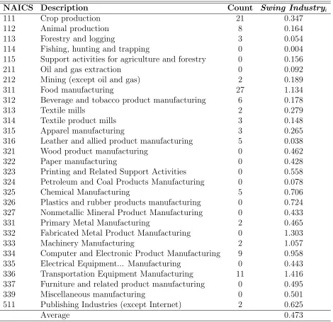
Table 1 lists the number of disputes filed in each sector over our entire sample. It also
provides information on the importance of each industry in swing states, captured by the
12Given that the variable is expressed as a share of total employment, there is no need to normalize it by
the number of swing states. Also notice that swing states are redefined every four years, after the Presidential elections. In our empirical analysis, we include President-term fixed effects, which account for changes in the number of swing states.
13A 4-digit NAICS industry is classified as tradable if its imports plus exports equal to at least $10,000
average of the Swing Industryi,t variable over our sample period. The statistics of Table 1
reveal a correlation between industry size in swing states and the incidence of WTO disputes.
For example, the maximum number of disputes (27) is found in food manufacturing, a sector
in which the average of Swing Industryi,t (1.134) is well above the average for the entire
sample (0.473). The simple correlation between the number of disputes filed in an industry
and its average size in swing states is 0.323. The correlation is much higher within 2-digit
[image:10.612.73.543.256.711.2]NAICS industries (e.g. 0.889 in sector 11 and 0.943 in sector 31).
Table 1: WTO disputes filed by the U.S., by NAICS 3-digit industries
NAICS Description Count Swing Industryi
111 Crop production 21 0.347
112 Animal production 8 0.164
113 Forestry and logging 3 0.054
114 Fishing, hunting and trapping 0 0.004 115 Support activities for agriculture and forestry 0 0.156
211 Oil and gas extraction 0 0.092
212 Mining (except oil and gas) 2 0.189
311 Food manufacturing 27 1.134
312 Beverage and tobacco product manufacturing 6 0.178
313 Textile mills 2 0.279
314 Textile product mills 3 0.148
315 Apparel manufacturing 3 0.265
316 Leather and allied product manufacturing 5 0.038 321 Wood product manufacturing 0 0.462
322 Paper manufacturing 0 0.428
323 Printing and Related Support Activities 0 0.558 324 Petroleum and Coal Products Manufacturing 0 0.078
325 Chemical Manufacturing 5 0.706
326 Plastics and rubber products manufacturing 0 0.724 327 Nonmetallic Mineral Product Manufacturing 0 0.433 331 Primary Metal Manufacturing 2 0.465 332 Fabricated Metal Product Manufacturing 0 1.303
333 Machinery Manufacturing 2 1.057
334 Computer and Electronic Product Manufacturing 9 0.958 335 Electrical Equipment... Manufacturing 0 0.443 336 Transportation Equipment Manufacturing 11 1.416 337 Furniture and related product manufacturing 0 0.495 339 Miscellaneous manufacturing 0 0.501 511 Publishing Industries (except Internet) 2 0.625
Average 0.473
To capture other industry determinants of the initiation of trade disputes, we include in
our analysis other variables defined at the same level of disaggregation as Swing Industryi,t
(3-digit NAICS). We follow Bown and Crowley (2013b) for our choice of political-economic
controls. To measure the importance of an industry in the U.S. at large, we construct the variable ln(Employmenti,t), which measures the total number of employees in industry i in
yeart. We also include ln(Concentrationi), which measures the total market share of the four
largest firms in an industry i. This variable is time invariant and is not available for
agri-culture.14 The variablesEmployment Growth Rate
i,t−1,Growth rate importsi,t−1 and Growth
rate exportsi,t−1 capture employment changes and the evolution of imports and exports in
industry iprior to the initiation of the dispute (between yeart−2 andt−1). The
employ-ment variable comes from the Bureau of Labor Statistics and is available for all years and
sectors. The industry trade variables are constructed using data from U.S. customs, which
only cover trade in goods.
One possible concern is that re-election year effects could result from omitted variables
that also peak in 1996, 2004, and 2012. To deal with this concern, we include two
macroe-conomic variables, which recent studies suggest might affect the filing of trade disputes: ∆
Unemploymentt−1 and ∆ Exchange Ratet−1.15 ∆Unemploymentt−1 is the change in the
an-nual U.S. unemployment rate from the Current Population Survey of the BLS. ∆ Exchange Ratet−1 is the growth rate of the trade-weighted U.S. dollar index of major currencies that
is calculated by the Federal Reserve Board of Governors.16
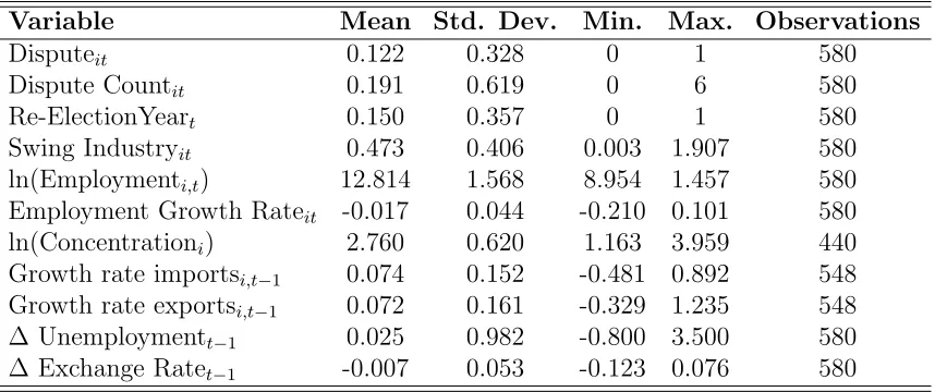
Table 2 provides summary statistics for the main variables used in our empirical analysis.
There were disputes in 71 (12 percent) of the industry-years. Three of the 20 years were re-election years. The table confirms that there is substantial variation in Swing Industryi,t,
our other main variable of interest, and the same is true for all the control variables.
Cross-tabulated data provide preliminary support for our hypotheses. We find that 24
percent of disputes filed by the U.S. occur in the three presidential re-election years, whereas
we would expect to find a 15 percent share (3 of 20) absent electoral cycles. Disputes occur
for 23 percent of industry-years in the top quartile of Swing Industryi,t, while they occur in
14The variable comes from the Annual Survey of Manufacturers of the U.S. Census Bureau and is only
available for 2002 and 2007. We use 2002, which is in the middle of our sample period.
15Bown and Crowley (2013a) find that nations refrain from applying temporary trade barriers against
nations with weaker macroeconomic conditions. These barriers are an important source of disputes, so a reduction in such barriers applied against the U.S. could explain a reduction in disputes filed by the U.S. We follow the authors’ choice of lagged macroeconomic indicators, albeit at an annual frequency rather than quarterly, and we use an index of U.S. exchange rates rather than bilateral exchange rates. Also, Li and Qiu (2014) find that disputes are pro-cyclical and that real exchange rates are a significant predictor of disputes.
16We also constructed the variable ∆GDP
t−1. However, since it is highly correlated (i.e. 0.76) with
∆Unemploymentt−1 and it is only available for part of our sample, we only include ∆Unemploymentt−1 in
just 9 percent of the industry-years in the bottom three quartiles.
Table 2: Summary statistics
Variable Mean Std. Dev. Min. Max. Observations
Disputeit 0.122 0.328 0 1 580
Dispute Countit 0.191 0.619 0 6 580
Re-ElectionYeart 0.150 0.357 0 1 580
Swing Industryit 0.473 0.406 0.003 1.907 580
ln(Employmenti,t) 12.814 1.568 8.954 1.457 580
Employment Growth Rateit -0.017 0.044 -0.210 0.101 580
ln(Concentrationi) 2.760 0.620 1.163 3.959 440
Growth rate importsi,t−1 0.074 0.152 -0.481 0.892 548
Growth rate exportsi,t−1 0.072 0.161 -0.329 1.235 548
∆ Unemploymentt−1 0.025 0.982 -0.800 3.500 580
∆ Exchange Ratet−1 -0.007 0.053 -0.123 0.076 580
3
Empirical analysis
In this section, we bring to the data two hypotheses motivated by the anecdotal evidence
cited in the introduction and later rationalized by our theory: (1) U.S. executives file more
trade disputes when they are close to re-election, and (2) trade disputes are more likely to target industries that are important to swing states in the presidential election.
We test these hypotheses using an industry-year panel. We present first our benchmark
results using a linear probability model, and then shown that our results are robust to using
alternative econometric methodologies.
3.1
Main results
To study the determinants of the initiation of U.S. trade disputes, we estimate the following
linear probability model:
Disputei,t =γ0+γ1 Re-Election Yeart+γ2 Swing Industryi,t+γ3 Xi,t+γ4Zt+γ5 Ii+εit (1)
where the dependent variable is the dummy variable Disputei,t, which is equal to 1 if the
United States files at least one dispute targeting industryi in yeart. The main variables of
interests areRe-Election YeartandSwing Industryi,t, which capture years and industries that
should be more important for a president’s re-election. The matrix Xi,t includes additional
industry-level controls, while Zt captures controls that vary over time only at the national
level. These includes macroeconomic variables, as well as fixed effects for each term served
by an executive or for his entire presidency.17 The panel structure of our data allows us to
include a matrix of industry fixed effectsIi at the two-digit level of the NAICS classification.
Tables 3 reports our main results. In column (1), we report the results of a parsimo-nious specification that includes only our key controls of interest, industry fixed effects, and
president fixed effects. In column (2), we add other additional industry-level and
country-level controls to account for other potential determinants of U.S. trade disputes. In this
specification, we only use controls that are available for all industries. In column (3), we
include ln(Concentration Ratioi). As mentioned in Section 2, this variable is time invariant
and is not available for agriculture sectors, so including it leads to a drop in the number of
observations. In column (4), we add the industry trade controls (Growth rate importsi,t−1
and Growth rate exportsi,t−1), which lead to a further drop in the number of observations.18
In columns (5)-(8), we reproduce the same specifications, substituting President fixed effects with President-term fixed effects.
The results of Table 3 confirm that U.S. trade disputes are “suspiciously-timed.” The
Re-Election Yeartdummy is always positive and significant at the 1 percent level, indicating
that U.S. executives are more likely to initiate disputes at the end of their first term, when
they are close to facing re-election. This result is robust to including President or
President-term fixed effects, as well as macroeconomic variables that might affect the timing of the
initiation of trade disputes. In terms of magnitude, the estimated coefficients for the Re-Election Yeartdummy indicate that the likelihood that the U.S. initiates a dispute increases
between 13.5 and 21.7 percentage points in the last year of a President’s first term
By including only theRe-Election Yeartdummy, we compare the last year of a president’s
first term with all other years. We have also tried to add the dummy Election Yeart, which
is equal to 1 in the last year of an executive’s second term. The estimated coefficient for
this dummy was never significant (while the Re-Election Yeart dummy remained positive
and significant at the 1 percent level), suggesting that the executive’s desire to retain office
is what drives the “suspicious timing” of U.S. trade disputes.
17Because of our interest in the variableRe-Election Year
t, we cannot include year fixed effects. President-term effects allow us to control for President-term-specific variables that may affect the initiation of disputes. In particular, they account for whether the executive can still be re-elected (first term) or faces term limits (second term). They also allow us to control for the number of swing states, which vary at the term-level.
Table 3: Linear Probability Model
(1) (2) (3) (4) (5) (6) (7) (8)
Re-Election Yeart 0.135*** 0.162*** 0.157*** 0.142*** 0.160*** 0.210*** 0.217*** 0.198***
(0.043) (0.048) (0.051) (0.051) (0.045) (0.055) (0.058) (0.059)
Swing Industryi,t 0.304*** 0.183*** 0.241*** 0.240*** 0.308*** 0.186*** 0.240*** 0.239***
(0.052) (0.064) (0.078) (0.079) (0.053) (0.064) (0.077) (0.078) ln(Employmenti,t) 0.063*** 0.055 0.056* 0.063*** 0.057* 0.059*
(0.018) (0.033) (0.034) (0.018) (0.032) (0.033) Employment Growth Ratei,t−1 -0.135 -0.285 -0.234 -0.145 -0.299 -0.311
(0.386) (0.506) (0.503) (0.384) (0.502) (0.501)
ln(Concentrationi) 0.138*** 0.139*** 0.139*** 0.140***
(0.025) (0.026) (0.025) (0.026)
Growth rate importsi,t−1 -0.145 -0.074
(0.115) (0.121)
Growth rate exportsi,t−1 0.024 0.032
(0.104) (0.108)
∆ Unemploymentt−1 -0.010 -0.004 -0.011 0.015 0.022 0.015
(0.017) (0.021) (0.021) (0.020) (0.025) (0.027) ∆ Exchange Ratet−1 0.336 0.277 0.184 0.384 0.398 0.309
(0.271) (0.302) (0.317) (0.381) (0.411) (0.416)
President FE yes yes yes yes
President-Term FE yes yes yes yes
Industry FE (2-digit) yes yes yes yes yes yes yes yes
Observations 580 580 440 428 580 580 440 428
R2 0.178 0.194 0.250 0.257 0.183 0.201 0.259 0.263
Notes: The table reports coefficients of a linear probability model, with robust standard errors in parentheses. ***, ** and * indicate statistical significance at the 1%, 5% and 10% levels respectively.
Our results about the Swing industryi,t variable suggests that electoral incentives also
affect the sectoral composition of the disputes filed by the United States. The estimated
coefficients for this variable are always positive and significant (at least at the 5 percent
level), indicating that industries that are more important in swing states receive more sup-port in fighting against violations of multilateral trade laws. Crucially, this result is robust
to controlling for the political importance of an industry in the country at large, by including
measures of its overall size and its degree of concentration. The variables ln(Employmenti,t)
and ln(Concentrationi) are both positive and significant, suggesting that the U.S. is more
likely to initiate trade disputes in support of larger and more concentrated industries. In
terms of magnitude, a marginal increase in the variableSwing Industryi,t increases the
prob-ability that a dispute is initiated by between 18.3 and 30.8 percentage points. If we compare
the effects of different industry determinants, we find that a 1 standard deviation change in
Swing Industryi,t increases the probability that a trade dispute is initiated by between 7.4
and 12.5 percentage points; by contrast, the effect is between 5.1 and 7.3 percentage points
for a 1 standard deviation increase in ln(Employmenti,t) and between 8.6 and 8.8 percentage
points for a 1 standard deviation increase in ln(Concentration Ratioi).
3.2
Robustness checks
3.2.1 Probit model
We first verify the robustness of our results to using a probit model as an alternative
econo-metric methodology. We estimate the following specification:
P r(Disputei,t = 1|·) = Φ(λ0+λ1 Re-ElectionYeart+λ2 Swing Industryi,t
+λ3 Xi,t+λ4 Zt+λ5 Ii) (2)
where Φ denotes the standard normal cumulative distribution function.
Table 4 displays the estimated probit coefficients. As with our benchmark regressions
of Table 3, the Re-Election Yeart dummy is always positive and significant at 1 percent,
confirming that U.S. executives are more likely to initiate trade disputes in the last year of
their first term. The estimated coefficient for Swing Industryi,t is also positive and
signifi-cant, confirming that trade disputes are more likely to involve important industries in swing
states.19
19Notice that the number of observations in columns (4) and (8) is lower than in the corresponding
Table 4: Probit Results
(1) (2) (3) (4) (5) (6) (7) (8)
Re-Election Yeart 0.684*** 0.925*** 1.084*** 1.009*** 0.890*** 1.283*** 1.681*** 1.556***
(0.186) (0.263) (0.323) (0.339) (0.233) (0.349) (0.450) (0.467)
Swing Industryi,t 1.482*** 0.763** 1.041** 1.022** 1.505*** 0.772** 0.995** 0.982*
(0.243) (0.321) (0.515) (0.520) (0.248) (0.317) (0.508) (0.514) ln(Employmenti,t) 0.430*** 0.374 0.400 0.439*** 0.434 0.451
(0.125) (0.278) (0.280) (0.121) (0.275) (0.277) Employment Growth Ratei,t -2.095 -3.307 -2.022 -2.155 -3.917 -2.936
(2.704) (2.990) (3.095) (2.705) (3.028) (3.158)
ln(Concentrationi) 0.916*** 0.918*** 0.953*** 0.952***
(0.165) (0.168) (0.172) (0.173)
Growth rate importsi,t−1 -2.073 -1.619
(1.518) (1.648)
Growth rate exportsi,t−1 -0.114 -0.008
(0.944) (1.011)
∆ Unemploymentt−1 -0.070 -0.030 -0.151 0.087 0.151 0.025
(0.123) (0.151) (0.165) (0.138) (0.170) (0.190) ∆ Exchange Ratet−1 2.570 3.064 1.958 2.672 4.510 3.393
(2.034) (2.545) (2.651) (2.670) (3.249) (3.292)
President FE yes yes yes yes
President-Term FE yes yes yes yes
Industry FE (2-digit) yes yes yes yes yes yes yes yes
Observations 580 580 440 420 580 580 440 420
Pseudo R2 0.240 0.266 0.345 0.357 0.249 0.276 0.363 0.369 Predicted Probabilities
ˆ
P(Re-Election Yeart = 0) 0.103*** 0.099*** 0.091*** 0.093*** 0.099*** 0.094*** 0.085*** 0.087***
(0.012) (0.012) (0.013) (0.013) (0.012) (0.012) (0.012) (0.013) ˆ
P(Re-Election Yeart = 1) 0.232*** 0.278*** 0.270*** 0.253*** 0.274*** 0.358*** 0.390*** 0.357***
(0.034) (0.057) (0.061) (0.060) (0.050) (0.083) (0.098) (0.097) ˆ
P(Swing Industryi,t= 25th pct) 0.063*** 0.082*** 0.065*** 0.066*** 0.063*** 0.082*** 0.068*** 0.068***
(0.010) (0.017) (0.018) (0.019) (0.010) (0.016) (0.018) (0.019) ˆ
P(Swing Industryi,t= 75th pct) 0.177*** 0.138*** 0.128*** 0.133*** 0.177*** 0.138*** 0.126*** 0.131***
(0.019) (0.016) (0.021) (0.024) (0.019) (0.016) (0.020) (0.023)
Notes: The first part of the table reports coefficients of a probit model, with robust standard errors in parentheses. The second part of the table reports the model’s average predicted probabilities, as we condition two variables in the ˆP(·) function taking on the specified values while the other variables are taking their actual values. ***, ** and * indicate statistical significance at the 1%, 5% and 10% levels respectively.
To help interpret the probit results, at the bottom of Table 4 we report the model’s
average predicted probabilities for different values of the variables Re-Election Yeart (0 or
1) and Swing Industryi,t (25th to the 75th percentile).20 All the predicted probabilities are
significantly different from each other (within each specification). Comparing the predicted probabilities across the different scenarios confirms that the U.S. is more likely to initiate
disputes in re-election years and that the disputes are more likely to involve important
industries in swing states. For example, the probabilities reported in column (1) indicate
that moving from a no re-election year to a re-election year increases the probability that a
dispute is initiated from 10.3 percent to 23.2 percent. Similarly, moving theSwing Industryi,t
variable from the 25th to the 75th percentile increases the probability that a dispute is
initiated from 6.32 percent to 17.7 percent (with similar patterns in the other columns).
3.2.2 Count Model
In order to exploit the variation from industries involved in more than one dispute in a given
year, we estimate a count model using Dispute Counti,t as the dependent variable.21 This
alternative methodology also provides an additional functional form check on our previous
results.
We assume Dispute Counti,t, conditional on the data, follows a negative binomial
distri-bution with parametersµit and α such that
E [DisputeCounti,t|·] =µi,t ≡exp(β0 +β1 Re-ElectionYeart+β2 Swing Industryi,t
+β3 Xit+β4 Zt+β5 Ii) (3)
and V ar[DisputeCountit|·] = µi,t +αµ2i,t. We then estimate this model using maximum
likelihood.
Table 5 provides the estimates of the negative binomial regressions. In all specifications,
the Re-Election Yeart dummy is positive and significant at the 1 percent level, confirming
that the U.S. executives are more likely to initiate WTO disputes in the year before their
re-election. The estimates of the Swing Industryi,t variables are also positive and significant
at least at the 5 percent level, confirming that the disputes filed by the U.S. are more likely
to involve important industries in swing states.
20When computing the predicted probabilities for different values of a variable of interest, we keep the
other variables at their actual values.
Table 5: Negative Binomial Results
(1) (2) (3) (4) (5) (6) (7) (8)
Re-Election Yeart 1.147*** 1.412*** 1.678*** 1.634*** 1.236*** 1.548*** 2.023*** 1.955***
(0.235) (0.353) (0.426) (0.448) (0.329) (0.472) (0.594) (0.615)
Swing Industryi,t 2.534*** 1.421*** 2.218*** 2.123** 2.573*** 1.475*** 2.227*** 2.15**
(0.364) (0.483) (0.812) (0.845) (0.371) (0.489) (0.845) (0.880) ln(Employmenti,t) 0.581*** 0.243 0.292 0.569*** 0.258 0.297
(0.191) (0.429) (0.438) (0.186) (0.426) (0.437) Employment Growth Ratei,t−1 -1.781 -1.638 -1.019 -1.704 -1.750 -1.336
(4.057) (4.480) (4.665) (4.181) (4.618) (4.858)
ln(Concentrationi) 1.062*** 1.064*** 1.071*** 1.075***
(0.194) (0.196) (0.198) (0.200)
Growth rate importsi,t−1 -1.414 -1.094
(2.138) (2.333)
Growth rate exportsi,t−1 -0.405 -0.274
(1.194) (1.248)
∆ Unemploymentt−1 0.007 0.113 0.005 0.143 0.277 0.174
(0.198) (0.223) (0.250) (0.220) (0.245) (0.277) ∆ Exchange Ratet−1 2.711 4.614 4.020 2.279 4.560 4.019
(2.947) (3.516) (3.624) (3.643) (4.356) (4.486)
President FE yes yes yes yes
President-Term FE yes yes yes yes
Industry FE yes yes yes yes yes yes yes yes
Observations 580 580 440 428 580 580 440 428
Pseudo R2 0.214 0.229 0.288 0.291 0.218 0.232 0.292 0.295 Predicted Counts
ˆ
C(Re-Election Yeart = 0) 0.147*** 0.143*** 0.125*** 0.127*** 0.145*** 0.140*** 0.122*** 0.123***
(0.021) (0.021) (0.020) (0.021) (0.021) (0.021) (0.021) (0.021) ˆ
C(Re-Election Yeart = 1) 0.464*** 0.586*** 0.669** 0.648** 0.499*** 0.659** 0.922* 0.872*
(0.092) (0.182) (0.261) (0.266) (0.134) (0.271) (0.502) (0.491) ˆ
C(Swing Industryi,t= 25th pct) 0.085*** 0.105*** 0.071*** 0.072*** 0.085*** 0.104*** 0.071*** 0.072***
(0.014) (0.023) (0.015) (0.016) (0.014) (0.023) (0.016) (0.017) ˆ
C(Swing Industryi,t= 75th pct) 0.320*** 0.220*** 0.212*** 0.215*** 0.324*** 0.224*** 0.213*** 0.218***
(0.056) (0.032) (0.069) (0.073) (0.057) (0.033) (0.071) (0.076)
Notes: The first part of the table reports coefficients of a negative binomial model, with robust standard errors in parentheses. The second part of the table reports the model’s average predicted counts, as we condition on specific valued of the variables in the ˆC(·) function taking on the specified values while the other variables are taking their actual values. ***, ** and * indicate statistical significance at the 1%, 5% and 10% levels respectively.
To get a sense of the magnitude of the effects in the negative binomial regressions, at the
bottom of Table 5 we report the model’s average predicted counts for different values of the
variables Re-Election Yeart (0 or 1) and Swing Industryi,t (25th to the 75th percentile). We
additionally test whether differences in predicted counts — corresponding to the re-election effect and the swing industry effect — are statistically different from each other. We find
both effects to be significant at the 5 percent level for columns (1), (2), (3), and (5) and at
the 10 percent level for columns (4) and (6). For columns (7) and (8), which consider the
more limited sample, the re-election and swing industry effects are still significant at the 10
percent level. On balance, the results continue to support the conclusion that the U.S. is
more likely to initiate disputes in re-election years and that the disputes are more likely to
involve important industries in swing states.
3.2.3 Instrumenting for the employment variables
The results presented so far provide systematic evidence supporting the existence of both
a re-election year effect and swing industry effect in U.S. trade disputes. To deal with
concerns about omitted variables, we have included in our regression many national-level
and industry-level variables which could be correlated with both the initiation of U.S. trade
disputes and our key variables of interest (Re-Election Yeart and Swing Industryi,t).
In this last section, we show that our results are also robust to a concern about reverse
causality. In particular, one may worry that the initiation of trade disputes involving a particular industry may affect its employment (in swing states and in the U.S. at large).
To address this concern, we use pre-sample data as instruments. Specifically, we
con-struct two instrumental variables, analogs for Swing Industryi,t and ln(Employmenti,t), but
constructed using employment data from 1994 and swing state classification from the 1992
election, so they vary only by industry. We then use a two-stage least squares estimation
which instruments for Swing Industryi,t and ln(Employmenti,t).
Table 6 shows the results from the two-stage least squares estimation.22 They are in line
with the results from the ordinary least squares estimation in Table 3 and provide a final
confirmation of our main hypotheses.
Table 6: Two-stage least squares regressions
(1) (2) (3) (4) (5) (6) (7) (8)
Re-Election Yeart 0.135*** 0.164*** 0.163*** 0.147*** 0.161*** 0.210*** 0.217*** 0.197***
(0.043) (0.048) (0.051) (0.051) (0.044) (0.055 (0.057) (0.058)
Swing Industryi,t 0.372*** 0.314*** 0.458*** 0.463*** 0.372*** 0.314*** 0.458*** 0.460***
(0.060) (0.079) (0.110) (0.112) (0.060) (0.080) (0.109) (0.111) ln(Employmenti,t) 0.025 -0.038 -0.042 0.025 -0.038 -0.040
(0.020) (0.043) (0.044) (0.020) (0.043) (0.044) Employment Growth Ratei,t−1 -0.179 -0.463 -0.374 -0.173 -0.448 -0.427
(0.392) (0.524) (0.520) (0.387) (0.512) (0.511)
ln(Concentrationi) 0.137*** 0.138*** 0.137*** 0.138***
(0.026) (0.026) (0.026) (0.026)
Growth rate importsi,t−1 -0.140 -0.0743
(0.113) (0.118)
Growth rate exportsi,t−1 -0.017 -0.001
(0.110) (0.113)
∆ Unemploymentt−1 -0.012 -0.011 -0.019 0.014 0.018 0.008
(0.017) (0.022) (0.023) (0.020) (0.025) (0.027) ∆ Exchange Ratet−1 0.366 0.367 0.254 0.374 0.397 0.296
(0.272) (0.308) (0.325) (0.380) (0.410) (0.414)
President FE yes yes yes yes
President-Term FE yes yes yes yes
Industry FE yes yes yes yes yes yes yes yes
Observations 580 580 440 428 580 580 440 428
R2 0.174 0.186 0.233 0.238 0.180 0.193 0.242 0.245
Notes: The table reports two-stage least squares coefficients, with robust standard errors in parentheses. The variables Swing Industryi,t and ln(Employmenti,t) are treated as endogenous. The first-stage instruments excluded from the second stage are analogs to the bolded variables, de-fined based on the level of employment in 1994. ***, ** and * indicate statistical significance at the 1%, 5% and 10% levels respectively.
3.3
Discussion
Our analysis confirms that disputes filed by the U.S. tend to be “suspiciously-timed”. In all
32 specifications of Tables 3-6 above, the Re-Election Yeart dummy is always positive and
significant at the 1 percent level, indicating that U.S. executives are more likely to initiate
disputes at the end of their first terms, when they are close to facing re-election.
In principle, there are three possible interpretations of this re-election year effect.
i) Some disputes were “delayed”, i.e. they should have been initiated earlier, but the
executive waited until the end of his first term, to maximize his re-election chances.
ii) Some disputes were pushed forward “too soon”, i.e. they would have been filed
any-way at some point in the future, but they were initiated earlier to boost the executive’s
re-election chances.
iii) Absent re-election motives, some disputes would not have been initiated at all.
Distinguishing between these interpretations is nontrivial. In line with interpretation
i), our results suggests that re-election motives, by delaying the filing of some disputes,
may imply a cost for the domestic industry involved. For example, as discussed further
in the conclusions, producers of car parts had to wait till September 2012 for the Obama administration to initiate a dispute against Chinese export subsidies to car parts, although
evidence of the existence of these subsidies had long been available.
The evidence does not seem instead consistent with interpretations ii). This would
sug-gest that disputes brought forward “too soon” by the executive should be weaker cases, i.e.
cases that the U.S. is more likely to lose. We have examined the outcomes of WTO disputes
from two perspectives and found no evidence that cases initiated in re-election years are
weaker.
First, we have looked at the status of the disputes, distinguishing cases that (a) are still
in consultations, (b) have been withdrawn or settled, and (c) have reached a panel. When comparing disputes filed in re-election years with disputes filed in other years, we found no
statistically significant difference in the distribution of outcomes.23
We have then looked at the outcome of the panels, using the database of Horn and
Mavroidis (2011) that classifies rulings through August 2011. Based on the “Conclusions
and Recommendations” section of each panel report, for each article cited in the dispute,
they classify the ruling into three categories: (1) claims where the complainant prevailed; (2)
23The percentage of cases that go to panel is actually higher for disputes filed in re-election year (53.85%
claims where the defendant prevailed; and (3) a residual group of claims where the outcome
is unclear. Summing up the outcomes, we classify outcomes as outright wins (defendant
never prevails), outright defeats (complainant never prevails), or mixed.24 Whether or not a
dispute was filed in a re-election year has no effect on the outcome: of the 8 disputes filed in re-election years that went to panel, 4 were outright victories and 1 was an outright defeat;
of the other 28 disputes that went to panel, 14 were outright victories and 2 were outright
defeats.
The evidence on the outcomes of trade disputes goes also partly against interpretation
iii). Assuming that the strongest cases are generally more likely to be filed, regardless of
re-election incentives, we would expect disputes that executives initiate only to remain in
office to be weaker cases. However, some disputes could still be consistent with interpretation
iii).25
Our results on the industry determinants of trade disputes suggest that re-election mo-tives distort not only the timing, but also the composition of disputes initiated by the United
States. In all our regressions, the variable Swing Industryi,t is positive and significant (at
least at the 5 percent level), indicating that the executives give more weight to voters in
swing states.
4
A model of electoral incentives and trade disputes
In this section, we describe a theoretical model that provides a simple explanation for our empirical findings concerning the timing of U.S. trade disputes (the re-election effect) and
their composition (the swing industry effect). The key assumption of this model is that
vot-ers have reciprocal preferences, i.e. they want to reward politicians who have been kind to
them, and punish politicians who have been unkind to them. As mentioned in the
introduc-tion, a large theoretical literature has emphasizes the importance of reciprocal preferences
(e.g. Rabin, 1993; Dufwenberg and Kirchsteiger, 2004; Falk and Fischbacher, 2006) and
many experimental studies have confirmed that individuals like to reward kind actions and
punish unkind ones (e.g. Fehr, G¨achter, Kirchsteiger, 1997; Charness and Dufwenberg, 2006;
Kube, Mar´echal, Puppe, 2012). Recent work by Finan and Schechter (2012) provides strong empirical and experimental evidence that voters exhibit reciprocal preferences.
The model is a sequential game between three actors: the incumbent politician, a
chal-24The outright wins and outright defeats include rulings in the residual category for only one dispute,
EC—Hormones, in which the complainant still prevailed for a majority of rulings.
25This could be the case if the likelihood of winning is the same across potential disputes, but for some
disputes the potential costs (legal, administrative, and political) would may then only be filed in re-election years, but would not be weaker cases in terms of the likelihood of the U.S. winning.
lenger, and the median voter. We first show that, if voters have standard preferences, their
decision will be driven only by ideology. In this scenario, electoral incentives will have no
impact on the filing of trade disputes. We then show that re-election motives can lead the
incumbent politician to file a trade dispute, if voters are not too ideological and have intrinsic reciprocal preferences, i.e. want to be (un)kind to an (un)kind politician.
4.1
Players, actions, and strategies
We assume that politicians can only serve two terms, lasting one period each. This
assump-tion allows us to study how the behavior of an incumbent politician varies between the first
period (when he can still be re-elected) and the second period (when he has no re-election
motives).
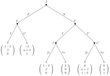
The model consists of three stages:
1. In the first period, the incumbent I decides whether to initiate a trade dispute against another WTO country. The incumbent’s action is denoted bymI. The incumbent can
choose between filing a complaint (action F) and not (actionN).
2. At the end of the first period, after having observed the electoral campaign, voters
decide who gets elected for the next term. In order to keep the model tractable, we concentrate on the median voter V. By slight abuse of notation, action I denotes the
vote for the incumbent, and action C the vote for the challenger C.
3. In the second period, the elected president can file a complaint, if it has not yet been filed by the incumbent in stage 1. In this case, the re-elected incumbent can choose
between filing a complaint (actionfI) and not (actionnI). If the challenger gets elected
and the former president has not filed the complaint in stage 1, the challenger has the
choice between fC and nC.
Denote the set of pure strategies of each player as AI ≡ {F fI, F nI, N fI, N nI}, AC ≡ {fC, nC}, and AV ≡ {II, IC, CI, CC}. For the incumbent strategy, the first character
denotes the stage 1 choice and the second denotes the stage 3 choice. For the voter strategy,
the first character is the action conditional on F, and the second is the action conditional
onN.
Denote a particular pure strategy of each politician as aI ∈ AI and aC ∈AC.26 Denote
a particular voter strategy as aV ∈∆(AV), the set of mixed strategies over AV. We further
26If we were to allow mixed strategies for the politicians, we would find that the politicians play only pure
Figure 2: Extensive form of the game with material payoffs for players I, V, and C
I
V
1−δ β 0 I −δ α+β
1 C F V I
1−δ β 0 fI 1 0 0 nI I C 0
α+β
1−δ fC 0 α 1 nC C N
denote a particular mixed strategy aV as pIC ·IC+pCC ·CC+pII·II+pCI ·CI. For any
mixed strategy we introduce, we denote the probabilities of its pure strategies with matching
superscripts, e.g. the probability of playingIC when choosing mixed strategya0V is denoted byp0IC.
See Figure 2 for the extensive form of the game. The figure depicts only the material
(direct) component of payoffs, omitting the voter’s reciprocal payoffs. We elaborate further
on both payoff components in the following subsection.
4.2
Payoffs
Politicians: We assume that politicians are office motivated, and earn a payoff of 1 when they are in office and a payoff of zero out of office.
A politician bears a cost of δ for initiating a trade dispute.27 Given our assumptions
about the politicians’ payoffs, if δ > 1, then the dispute will never be filed. By contrast, if
δ <0, the dispute will always be filed. Many potential disputes fall into these categories, such
27A priori it is unclear whether a complaint is also costly when the other politician files the complaint. For
this model we have chosen that only the politician filing the complaint has to bear the cost. Hence,δreflects the political costs of a complaint, and not an intrinsic preference of the politicians. None of our results would change if the complaint is also costly when the other politician files it. One might also speculate that the costs of filing a complaint might be different for the incumbent and the challenger. Again, none of our results would change as long as the costs are strictly positive for both politicians.
that re-election incentives would not matter. We focus on the parameter range δ ∈ (0,1),
for which re-election motives may affect politicians’ choices.
Our assumption that politicians bear some costs when filing trade disputes warrants
some discussion about the possible sources of such costs. The literature points out that there are the direct costs of litigating a dispute, as successful disputes require significant
legal expertise. For example, Bown (2009) cites estimated litigation costs exceeding 10
million US$ for individual disputes. Disputes can also have a shadow cost, due to limited
resources at every stage of the dispute process (see Chapter 5 of Bown, 2009, for details on
the process). Such dispute costs have played a significant role in prior theory of the WTO
dispute settlement process. Maggi and Staiger (2011) argue that a dispute cost is important
for explaining a pro-trade bias in WTO rulings.
Voters: The payoff of the voter consists of two parts. First, there is a material (direct) payoff, depending on the strategies of the politicians and on his vote. This payoff is denoted
by πV(aI, aV, aC). It is normalized to zero when the incumbent gets re-elected and no
complaint is filed. We use α to denote the median voter’s additional material payoff if the
challenger gets elected. If α is positive, the median voter has an intrinsic preference for the
challenger. If α is negative, he has an intrinsic preference for the incumbent. Note that the
smaller the absolute value of α, the “closer” the race in the respective state and the more
important the trade issue in relative terms. We useβto denote the median voter’s additional
payoff from a complaint. We assume β >0.
In addition to the material payoff, the voter is motivated by reciprocity, i.e. the desire to choose an action that is (un)kind to an (un)kind politician. Following the preference form
of Dufwenberg and Kirchsteiger (2004), we will denote the voter’s reciprocity toward each
of the two politicians as the product of two concepts to be defined: (1) the voter’s kindness
toward the politician, and (2) the voter’s perception of the politician’s kindness to the voter.
The voter’s utility is the sum of the reciprocity payoffs for each politician and the material
payoff.
A strategy choice of player i is kind to another player j if the choice intends to give j
a high material payoff, minus the average between the highest and the lowest payoff i can
intend give to j. The payoff the voter intends to give to a politician by choosing a particular strategyaV depends on the incumbent’s first stage actionmI, which the voter already knows
when making a choice in stage 2. The intended payoff also depends on the choices made in
stage 3 (if the incumbent has chosen N in stage 1) which the voter does not know when he
makes his choice. Hence, the voter has to form beliefs about what will happen in stage 3.
Denote by bI ∈ {fI, nI} the voter’s belief about the incumbent’s action in stage 3, and by
to politicians I and C bykI(aV |mI, bI, bC) and kC(aV |mI, bI, bC) respectively.
What is the kindness of a politician to the voter, as perceived by the voter? It is the
material payoff the voter thinks that the respective politician intends for the voter, minus
the average of what the voter thinks is the maximum and the minimum the politician can intend for the voter. The material payoff the voter thinks that the incumbent intends for
him depends on the stage 1 actionmI of the incumbent, and on the voter’s first order beliefs
about the politicians’ stage 2 actions, bI and bC. The voter’s material payoff depends of
course also on the voter’s strategy. The material payoff the incumbent can intend for the
voter depends also on the incumbent’s belief about the voter’s strategy. For measuring the
voter’s perception about the incumbent’s intentions we need cI
V, the voter’s second-order
belief about the incumbent’s belief about the voter’s strategy. Due to a similar reasoning,
the voter’s second-order belief about the incumbent’s belief about the challenger’s strategy,
denoted by cIC, is required. Denote the voter’s perception of the incumbent’s kindness to the voter by κI(mI, bI, bC, cIV, cIC). For a similar reason, the voter’s perception of kindness
of the challenger’s strategy choice depends on the first-stage action of the incumbent mI,
on the first-order beliefs of the voter, bI and bC, on the voter’s second-order belief about
the challenger’s belief about the voter’s strategy, cC
V, and on the voter’s second-order belief
about the challenger’s belief about the third-stage action of the incumbent, cC
I. Denote the
voter’s perception of the challenger’s kindness by κC(mI, bI, bC, cCV, cCI).
The overall utility of the voter choosing strategy aV is
uV(aI, aV, aC, bI, bC, cIV, c I C, c
C V, c
C
I) = πV(aI, aV, aC)+ (4)
kI(aV |mI, bI, bC)κI(mI, bI, bC, cIV, c I
C) +kC(aV |mI, bI, bC)κC(mI, bI, bC, cCV, c C I).
This formulation implies that the voter wants to behave reciprocally, and that this wish to
be kind (unkind) to a certain politician increases with the perceived kindness (unkindness)
of the politician to the voter.
Notice that the reciprocity payoff also depends oncI
V, the voter’s belief of the incumbent’s
perception of the voter’s behavior. In equilibrium (which we later define), this beliefcI V must
be consistent with the voter’s behavior. We later show that for certain parameter ranges, the
dependence of the voter’s payoff oncIV leads to a unique equilibrium in which the voter plays
a mixed strategy. Unlike typical mixed strategy equilibria, in which each player’s mixed
strategy implies the other players’ indifference, here a belief cIV consistent with a mixed strategy can imply the voter’s indifference between candidates for at least one decision node.
For example, if the voter materially prefers the challenger and cI
V = IC, then the
per-ceived kindness of an incumbent’s dispute is mitigated, because the voter recognizes that the
incumbent fully anticipates that his dispute would cause the voter to choose counter to the
material preference. If this reduction in perceived kindness would lead the voter to prefer
strategy aV of CC rather than IC, then there cannot be a pure strategy equilibrium with
belief cIV = IC, because that belief would be inconsistent with the voter’s preference. But there can be an equilibrium involving a mixed strategy between CC and IC, such that for
cI
V consistent with this mixed strategy, the voter is indifferent between candidates when the
incumbent files a dispute.
4.3
Kindness calculations
Here we give examples of kindness function evaluation. The example calculations are chosen
to be useful in the next subsection. Throughout this subsection, we assume that the voter
expects no stage 3 disputes, i.e. bI = nI and bC = nC. We also assume, unless otherwise
indicated, that the voter believes that neither candidate anticipates that the other will file
a dispute in stage 3, i.e. cIC =nC and cCI =nI.
Kindness of the voter to the politicians: First, assume that the incumbent has chosen
N in stage 1. With such beliefs and knowing that mI = N, choosing II or CI gives
the incumbent a material payoff of 1, which is the maximum the voter could give to the
incumbent. Choosing II orCI gives the challenger 0, which is the minimum the challenger
could get. Choosing IC or CC gives the incumbent 0 (the minimum possible) and the
challenger 1 (the maximum possible). Suppose the voter plays the strategyaV =pIC·IC+
pCC·CC +pII ·II+pCI ·CI. Then,
kI(aV |N, nI, nC) =pII +pCI −
1
2(1 + 0) =pII +pCI − 1
2. (5)
kC(aV |N, nI, nC) =pCC +pIC −
1
2(1 + 0) =pCC+pIC − 1 2.
If the incumbent instead chooses F in stage 1, then
kI(aV |F, nI, nC) =pIC +pII−δ−
1
2((1−δ) + (−δ)) = pIC +pII − 1
2. (6)
kC(aV |F, nI, nC) =pCC +pCI −
1
2(1 + 0) = pCC+pCI − 1 2.
To summarize, a pure strategy of the voter yields a kindness of 12 to the election winner
and a kindness of −1
2 to the election loser, where the election outcome is conditional on
the voter’s strategy and the incumbent’s first-stage action. For the mixed strategies, the