warwick.ac.uk/lib-publications
Original citation:
Cormode, Graham and Hickey, Christopher (2018) Cheap checking for cloud computing :
statistical analysis via annotated data streams. In: The 21st International Conference on
Artificial Intelligence and Statistics, Playa Blanca, Lanzarote, Canary Islands, 9-11 Apr 2018.
Published in: Proceedings of the 21st International Conference on Artificial Intelligence and
Statistics, 84
Permanent WRAP URL:
http://wrap.warwick.ac.uk/99395
Copyright and reuse:
The Warwick Research Archive Portal (WRAP) makes this work by researchers of the
University of Warwick available open access under the following conditions. Copyright ©
and all moral rights to the version of the paper presented here belong to the individual
author(s) and/or other copyright owners. To the extent reasonable and practicable the
material made available in WRAP has been checked for eligibility before being made
available.
Copies of full items can be used for personal research or study, educational, or not-for-profit
purposes without prior permission or charge. Provided that the authors, title and full
bibliographic details are credited, a hyperlink and/or URL is given for the original metadata
page and the content is not changed in any way.
Publisher’s version:
Proceedings of the 21st International Conference on Artificial Intelligence and Statistics
(AISTATS) 2018, Lanzarote, Spain. PMLR: Volume 84. Copyright 2018 by the author(s).
A note on versions:
The version presented here may differ from the published version or, version of record, if
you wish to cite this item you are advised to consult the publisher’s version. Please see the
‘permanent WRAP URL’ above for details on accessing the published version and note that
access may require a subscription.
Statistical Analysis via Annotated Data Streams
Graham Cormode Christopher Hickey
University of Warwick
Abstract
As the popularity of outsourced computation in-creases, questions of accuracy and trust between the client and the cloud computing services be-come ever more relevant. Our work aims to pro-vide fast and practical methods to verify anal-ysis of large data sets, where the client’s com-putation and memory costs are kept to a mini-mum. Our verification protocols are based on defining “proofs” which are easy to create and check. These add only a small overhead to re-porting the result of the computation itself. We build up a series of protocols for elementary sta-tistical methods, to create more complex proto-cols for Ordinary Least Squares, Principal Com-ponent Analysis and Linear Discriminant Analy-sis, and show them to be very efficient in practice.
1 Introduction
The massive leap in popularity of machine learning tech-niques can be attributed in part not simply to novel al-gorithms, but also to dramatic increases in scale: much larger models with many parameters to set optimally, and much larger training data sets to determine these parame-ters. However, this presents a challenge to data owners who do not have a convenient data centre at their disposal. The size of data and computational cost in order to extract ac-curate models begins to look prohibitive. At the same time, a potential answer has emerged, in the form of outsourced computation. That is, instead of building the infrastructure needed to store and analyse large quantities of data, compu-tation can be ‘rented’ on demand. Initially cloud offerings provided only the barebones of a remote system, but cur-rent options provide many tools, libraries and algorithms available to take “off the shelf”.
Proceedings of the 21st International Conference on Artificial
Intelligence and Statistics (AISTATS) 2018, Lanzarote, Spain. PMLR: Volume 84. Copyright 2018 by the author(s).
One doubt remains. If we send data off to the cloud, and request some analysis to be performed, what guarantee do we get that the processing has been done to our satisfac-tion? The provider has an economic incentive to cut cor-ners: to perform the computation on only a sample of pro-vided data, or to terminate an iterative parameter search before convergence has occurred, for example. Such short cuts yield plausible but suboptimal models. So how could we be assured that the best model has been found, with-out repeating the computation ourself or having multiple providers repeat the work, substantially driving up costs? In this paper, we adopt the Annotated Data Streams ap-proach (Chakrabarti et al., 2009) for verifying the models found by an outsourced provider Rather than repeating all or some of the computation, we instead provide protocols in which the cloud also provides some extra information that allows us to check a strict adherence to the required computation. The overhead for the cloud provider is min-imal – often, the required information is a relatively low cost function of the input data or natural by-products of the target computation. These do not restrict the cloud to use any particular implementation or algorithm; just that they demonstrate that the output meets certain necessary properties. The key part of these protocols is that the in-formation required is very easy for the original data owner to check, based on appropriately defined fingerprints of the input. These fingerprints can be computed flexibly and in-crementally from the input as it arrives in any order, so the data owner does not even need to retain a complete copy of the input. The overhead for the data owner is therefore low: it is typically dominated by the cost of sending the data to the cloud and receiving the output of the computa-tion. If the data owner’s checks pass, then they are assured that the computation has been performed by the cloud sat-isfactorily, with a very high degree of certainty. One can then think of these protocols as providing effective “check-sums for computation”.
verifier corresponded exactly to the powerful class of com-putations that could be performed using polynomial space (PSPACE) (Babai, 1985; Goldwasser and Sipser, 1986; Shamir, 1992). Such results were initially thought to be of purely theoretical interest. A decade ago, this topic was re-visited from a perspective closer to our own: to what extent could arbitrary programs be checked without fully repeat-ing them (Goldwasser et al., 2008)? Several strong models were proposed, allowing a large class of computations to be checked in this way. However, the costs were still typically large: programs have to be compiled into non-standard for-mats (such as circuits with gates performing arithmetic op-erations), and the overheads for the cloud can be very sub-stantial, often hundreds or even millions of times slower than directly performing the computation.
We break away from this paradigm, and achieve protocols that have minimal overheads by deliberately narrowing the scope of the computations considered. By focusing on a collection of important tasks in machine learning based on linear algebra, we can provide bespoke protocols based on “fingerprinting” the input data that take advantage of specific structure in the target problem. These problems are of sufficient generality that our efforts are repaid. Af-ter surveying prior work and providing a technical back-ground (Section 2), we begin with primitives for ubiqui-tous steps in data analysis: matrix multiplication and inver-sion, Cholesky decomposition and eigenvalue finding (Sec-tion 3). In Sec(Sec-tion 4, we present applica(Sec-tions of these to tasks of interest: regression, PCA, and LDA. These core tasks are sufficient to show the power of this paradigm. We provide empirical validation of our claims in Section 5. This work represents some first steps in verifying out-sourced computation of machine learning. The next steps are to extend this work to more complex models and algo-rithms currently enjoying popularity in machine learning, such as deep learning and beyond. Since, at the risk of drastic oversimplification, almost all of machine learning can be performed via numerical data encodings (vectors, matrices and tensors) combined with optimization, we are optimistic that the foundations laid in this work will nat-urally extend to further protocols for common mining and modelling tasks.
2 Preliminaries
2.1 Annotated Data Stream Model
In our protocols, we have a data stream S, which is ob-served by two parties, a “helper” (H) and a “verifier” (V). The data stream will usually be arranged as a sequence of
ntuples of elements, where each tuple typically defines an element of a larger structure, such as a matrix or vector. Abstractly, the verifier wishes to compute some function onS,f(S), with assistance from the helper. Typically, the
helper will provide the value off(S), along with a proof
of its correctness. This yields theAnnotated Data Stream
model, introduced by Chakrabarti et al. (2009). We formal-ize the model via the definitions below.
Definition 1. We have a helperH, and a verifierV, with
the aim of cooperating to compute some function f(S)of the streamS. The helper provides a messageMH(S) com-prised of ,fˆ, the claimed valuef(S), and a proofPHwhich
supports this claim according to some pre-agreed structure. The output ofV based on the streamS,V’s randomly
cho-sen bitsRV, and the helper’s message is
OutV(S,RV, MH(S)) = (
ˆ
f IfV is convinced
⊥ Otherwise
A protocol is defined by the functionsMH andOutV. We say that a protocol iscompleteif
∃H :P[OutV(S,RV, MH(S)) =f(S)] = 1 (1)
The Verifier’s protocol issoundif
∀H0,S0:PhOut
V(S0,RV, MH0(S0))∈ {/ f(S0),⊥}
i ≤ 1
3
Intuitively this says that we seek protocols so that an honest helper (one who faithfully follows the protocol) can always persuade the verifier to accept the correct answer, while a dishonest helper cannot persuade the verifier to accept an incorrect result with more than a constant probability. Our protocols allow this probability to be reduced to an arbitrar-ily small value with minimal cost.
In order to show an annotated data streaming protocol, we need to show completeness and soundness. This is suffi-cient to check that our protocol will successfully do what we want: verify the computation with a high probability of detecting a malicious helper. Trivial protocols always exist wherein the helper’s message is null, and the verifier evaluates the function in full. Consequently, we seek proto-cols whose costs for the verifier are substantially lower than this. Ideally, the protocol should run in sublinear memory space for the verifier, without the need for intensive com-putation and the message should be as small as possible. Similarly, we seek protocols where the honest helper does not have to do substantially more work than simply com-puting f(S). Our focus in this paper are on the memory
space for the verifier, and the size of the proof, which we call the communication cost.
Definition 2. A (h,v)-protocol is a valid annotated data streaming protocol using a message of sizeO(h), andO(v)
space cost for the verifier.
2.2 Fingerprint techniques
Finite Fields.In line with prior work, all our protocols rely on computations performed over finite fields. For ease of implementation, we use prime fields. Given a primeq, the finite (prime) fieldFq is the set{0. . . q−1}with addition and multiplication moduloq. Hence, storing field values re-quiresO(logq)bits. We make use of the fact that in many cases arithmetic in the field and arithmetic over the integers is in exact correspondence. However, as we consider more complicated computations, we encounter situations where we seek solutions over the reals, which do not correspond to solutions in the field. To avoid this, we will use scaling and rounding techniques to approximate using field values. Specifically, we consider the input to be fixed precision ra-tional numbers which can be represented as members of the set Fρ,M = {x ∈ R∩[−M, M] : bρx ∈ Z}, with respect to a base, b. We then choose the field sizeqas a
function ofρandM, in order to allow us to maintain the
exact correspondence between the field and the fixed pre-cision rationals. We map y ∈ Fρ,M toy0 ∈ Fq, where
y0 = mod (xbρ, q), choosingqto be a prime bigger than
(2M+ 1)bρ.
Fingerprints.Most of the values stored by our verifier will be fingerprintsof large objects, such as vectors or matri-ces. Fingerprints (based on randomly chosen seedsx) have
the property that if two fingerprints agree, then with high probability the objects that gave rise to the fingerprints are identical.
Definition 3(Matrix fingerprint). ForA∈Fn×m
q , the ma-trix fingerprint of A isfmat
x (A)withx∈RFq and
fmat
x (A) = Pn−1
i=0
Pm−1
j=0 Aijxin+j
From the Schwartz-Zippel Lemma (Shamir, 1992), we have that for a randomly chosen x ∈ Fq, given A, B ∈
Fn×m
q , if A 6= B, then Pr[fx(A) = fx(B)] ≤ nmq−1. Therefore for sufficently large q(say, greater than 3nm)
we will always have soundness and completeness for ver-ifying equality with fingerprints. We can view vectors as a special case of matrices, so similarly for vectorsu∈ Fq we use the notationfvec
x (u) = Pn−1
i=0 uixito denote a
vec-tor fingerprint. Fingerprints have several useful properties, such as linearity, withfx(A+B) =fx(A) +fx(B).
2.3 Related Work
We briefly survey the most related work in this area. Chakrabartiet al.(Chakrabarti et al., 2009) introduced the annotated streams model and provided protocols for fre-quency moments in data streams, and several graph prob-lems, including triangle counting, connectivity and bipar-tite matchings. They also introduced a square matrix mul-tiplication protocol built extending the classical result of Freivalds (1979). Subsequently, Cormode et al. (2013) pro-vided further protocols for graph problems, using linear and integer programs to validate optimal matchings and
shortest paths. More recently, Daruki et al. (2015) extended results on matrix analysis, provided more general protocols for matrix multiplication, and a protocol for eigenvalue (but not eigenpair) checking. For matricesA∈Fk×n
q andB ∈
Fn×k0
q , they show an (kk0hlog(q), vlog(q))−protocol, where hv ≥ n. These protocols are used to perform
shape fitting and clustering, although they shift away from annotated data streams and towards an interactive proof model which allows several exchanges of messages be-tween helper and verifier. The annotated data stream model is generalized by definitions ofstreaming interactive proofs
(SIPs) (Cormode et al., 2011, 2012). Note that annotated data stream verification protocols can be considered as sin-gle message SIPs.
3 Linear Algebraic Checks
In this section, we define protocols for checking a variety of linear algebraic primitives, based on careful use of fin-gerprints. We use the notationA→
i to denote theith row of the matrixA, andA↓i to denote theith column ofA.
3.1 Fingerprinting the Gramian Matrix
We first show how to efficiently build a fingerprint of the Gramian matrixG=ATAgiven a stream that specifiesA.
Lemma 1. ForA∈Fn×m q ,
fmat
x (ATA) =Pni=1fxvecm(A→i )fxvec(A→i )
Proof. Givenp, q∈Fm q ,
fmat
x (p⊗q) = Pm−1
i=0
Pm−1
j=0 piqjxim+j
=Pmi=0−1piximPmj=0−1qjxj
=fvec
xm(p)fxvec(q)
,
Using the outer product definition of matrix multiplication;
fmat
x (ATA) =Pn−
1
i=0 fxmat
(AT)↓
i
(A→
i )
=Pni=0−1fvec
xm(A→i )fxvec(A→i )
Hence, we can compute the fingerprint of ATA from A row-by-row and summing the product of row vector finger-prints. This immediately implies a protocol to verify that a matrixGprovided byH is the Gramian: simply use the above identity to computefx(ATA)from the stream, and check that this is equal tofx(G). Soundness and complete-ness follow immediately from properties of fingerprints in Section 2.2, and the cost isO(m2logq)communication to
specifyG, while the verifier can maintain the needed fin-gerprints in spaceO(logq).
3.2 Matrix Multiplication
We generalize the previous protocol to solve matrix multi-plication. Given two matrices,A∈Fk×n
q andB ∈Fn×k
0
a similar proof to Lemma 1 shows
fxmat(AB) = nX−1
i=0
fxveck0(A↓i)fxvec(Bi→) (2)
Equation (2) allows for an efficient matrix multiplication protocol, where the main work of the helper is to repeat the input matrices in a convenient order. To find the fingerprint ofABwe need to see each column of A and row of B
in-terleaved in order, i.e. MH =hA˜↓0,B˜→0 , ...,A˜↓n−1,B˜n→−1i.
The verifier uses fingerprints to check that the reordered versions ofAandBagree with the versions present in the
streamS, and that the claimed matrix productC has the
same fingerprint as the fingerprint computed via (2).
Theorem 1. There is a (max(k0k, kn, k0n) log(q),
log(q))-protocol for verifying matrix multiplication with
A∈Fk×n
q ,B ∈Fn×k
0
q .
Soundness and completeness are again immediate from the properties of fingerprints. The verifier keeps a constant number of fingerprints in space O(log(q)), and the
com-munication cost ofO(max(k0k, kn, k0n) log(q))is due to
sending each ofA,BandAB.
Matrix multiplication has been considered in prior work on annotated streaming. Daruki et al. (2015) showed that any protocol for this problem must have the product of the communication cost and space cost at leastΩ((k+k0)n).
Our protocol achieves this lower bound up to logarithmic factors (noting that any protocol which reports(AB)
re-quiresΩ(kk0)communication for this step). The previous
best rectangular matrix multiplication protocol, achieved by Daruki et al. (2015), was a kk0hlog(q), vlog(q)
-protocol with hv ≥ n, that used the inner product
proto-col of Chakrabarti et al. (2009). Our protoproto-col can be un-derstood as settingv = 1, but removing the high overhead
factor ofnfrom the communication cost in this case. When
our input matrices are constituted of fixed precision ratio-nals, we chooseqas follows:
Corollary 1. GivenA∈ Fρ,Mk×n andB ∈ Fρ,Mn×k0, the ma-trixABis inF2nρ,nM×n 2, and we chooseq > n(2M+ 1)222ρ
so that the product can be represented exactly in the field.
Choosing q to be this large means that when we move A and B from Fρ,M to A,˜ B˜ ∈ Fq by multiplying by
2ρ, and then computeA˜B˜ all these values remain in F q, and by scaling back down by 22ρ we get our result in the desired format, without wraparound or rounding er-rors. The memory required to store elements of Fq is
log(q) = O(log(M) + log(b)ρ), which is proportional to
the space required to store the original matrices inFρ,Mis
log(M) + log(b)ρ.
Lower bounds on computing matrix fingerprints. The verifier needs very little memory for the above protocol, since the matrix is provided in a convenient order. More
generally, we would like to be able to findfxmat(AB)from justfmat
x (A)andfxmat(B), without requiring the helper to repeat these. This would reduce communication and sim-plify the protocol; however, we show this is not possible.
Theorem 2. Any functiongwithfmat
x (AB) =g(fxmat(A),
fmat
x (B))forA, B∈Fnq×nrequires that fingerprintsfxmat are at leastΩ(n)bits in size.
Proof. We make use of a hard problem from communica-tion complexity to show the space lower bound. In the DIS-JOINTNESSproblem, two players Alice and Bob each have a bit string,a,b ∈ {0,1}n, and they wish to see whether for anyi ∈[n]they haveai =bi = 1. If we had a func-tionfmat
x : Fnq×n →Fq they could createn×nmatrices A and B withaandbon the diagonals and 0’s elsewhere.
Then Alice could send Bobfmat
x (A), Bob could compute
fmat
x (B), and then find fxmat(AB) using g.Observe that
AB = 0iff stringsaandb are disjoint, and is non-zero
otherwise. So by comparing fxmat(AB)to fxmat(0), we can determine the answer to the disjointness problem. The fingerprints must be at leastΩ(n)bits from the correspond-ing communication complexity ofDISJOINTNESS(H˚astad and Wigderson, 2007).
3.3 Eigenvalue Check
For the subsequent problems, we need to apply scaling and rounding, as mentioned earlier. There is a tension here, since matrix computations can include values which are very large compared to the input values. We also need to ensure that our approximation tolerance always allows an honest helper to find a satisfying answer, but prevents a dis-honest helper from getting a wildly wrong answer accepted. We first work with (approximate) eigenvectors and eigen-values of a symmetric matrix, i.e. a matrix such that ∀i, j. Aij = Aji. We wish to find pairs (λi, vi)over the reals, for alli ∈ [n], such thatAacts on each of the vec-tors by only scaling them by λi and that the vectors are orthonormal, i.e.
Avi=λivi vTi vj=δij = (
0 i6=j
1 i=j
Mapping these eigenpairs to the finite field can be deli-cate, since they may not align with coordinates in the field. Our protocol relies on a scaling factor T, which is used
to multiply up values from the original domain. The field size qmust grow by a corresponding factor to accommo-date the large range of values. To tolerate this, we relax to allow approximate eigenvectors as defined below. We first show that rounding to the scaled field FT q is always possible. Consider a particular eigenvector vi, and write
b
vi = T vi+r, withrj ∈ −21,12, andλbi = T λi +ρ, whereρ∈−1
2, 1 2
Theorem 3. For symmetricA ∈ Fn×n
q if(λi, vi), for all
i ∈ [n]are the eigenpairs ofA andvbi = T vi+r, with
r∈−1 2,
1 2
n
,λbi=T λi+ρforρ∈−12,12, then (inR)
|T Avbi−λbivbi| ≤
T nkAkF+
T√n
2 +
n
4
|vbiTvbj−T2δij| ≤ l
T√n+n 4
m
These bounds show how the error scales with the rounding factorT. To better interpret this, we next show that this
error can be made arbitrarily small by increasingT.
Theorem 4. If we have
|T Avbi−λbivbi| ≤
T nkAkF+T √n
2 +
n
4
|vbiTvbj−T2δij| ≤ l
T√n+n 4
m
Then we have (inR)
|T λi−λbi|
T ≤
2n√nkAkF
T +
n T +
n√n
2T2 :=EA,n(T)
andEA,n(T)→0asT → ∞
This means that if we want to find eigenvalues within cer-tain error, we simply have to check that the bounds of The-orem 4 hold, using a T∗ satisfying As kAkF = Ω(1), this expression isO(n3/2kAkF
T ). Hence it suffices to pick
T =O(n3/2
kAkF/).
Theorem 5. There is an annotated steaming
n2logqn3
2kAkF/
,logqn32kAkF/
−protocol for finding the eigenvalues of a symmetric matrix
A∈Fn×n
q to a precision of >0.
Proof. The protocol is relatively straightforward. The ver-ifier can computekAkF and a fingerprint ofA as the in-put is received. The helper provides the claimed matrix of (approximate) eigenvectorsV and corresponding
eigen-values D We then make use of the matrix multiplication
protocol to compute (T A −D)V. If the eigenvectors were exact, this would be 0; since they are approximate, we allow each entry in the result matrix to be at most
T nkAkF +12T√n+14n(computed over the reals and rounded to the finite field), and can verify that each entry of the product satisfies this bound. We also need to check that the eigenvectors are (almost) orthogonal, that is that each entry of(VTV
−T2I)is at mostT√n+1 4n
. Thus we need two invocations of the matrix multiplication proto-col, evaluated over a sufficiently large finite field. SettingT
according to the above bounds gives the claimed costs.
Once again, we consider the consequences of our input be-ingA∈ Fρ,Mn×n, and choose the value ofqas follows
Corollary 2. Given A ∈ Fρ,Mn×n and desired precision
, our matrices V and D are in F2nρ×0,nMn 2, where ρ0 = max{ρ,−log}. Therefore, to keep a direct
correspon-dence between verification done in the field, and our real values, we chooseq > n2(2M+ 1)222ρ0.
This value ofqis determined by the matrix multiplication
step, and the fact that the largest possible eigenvalue ofA
is bounded byn||A||max, where||A||maxisM.
3.4 Matrix Inversion
For matrix inversion we again scale the field by a factor
T. Over this expanded field, given ann×nmatrixA, we
want to find a matrixBsuch thatAB=T I. To allow for
rounding, we can relax the requirement of exact equality, and instead seek a matrixBthat acts approximately like an
inverse. We first show that such a matrix is guaranteed to exist.
Lemma 2. For an invertible A ∈ Fn×n
q , we can find a matrixB∈FnqT×nsatisfying
||AB−T I||max≤T (3)
ifT ≥ n2||A||max
2 and >0
Proof. Consider the true inverse ofA,A−1, computed over
the reals. Then we can find B = T A−1 +E so that B ∈ Zn×n and
∀i, j.|Ei,j| ≤ 12. We can then map the entries ofBdirectly into the fieldFT q. We then have
kAB−T Ikmax≤ kAEk2≤ 12n2kAkmax
That is, the error is at most n2 kAkmax
2T . We can set the pa-rameterTto be as large as needed to make this error value
some smallat quite modest cost: the field values are
rep-resented usingO(logn+ logkAkmax+ log 1/)bits.
Theorem 6. There is a streaming interactive
n2log(n
||A||maxq/),log(n||A||maxq/)-protocol to invert an invertible matrix A ∈ Fn×n
q with the above criteria,(3).
Proof. The protocol is based on the above Lemma: we require the helper to provide such a matrix B under the extended field FT q, along with the claimed value of AB. We then run the above protocol for matrix multiplica-tion, and check that each entry of AB meets the
re-quired size bound. This ensures that the rere-quired con-dition on entries is met. The cost of storing the fin-gerprints is O(log(nkAkmaxq/)), and the
communica-tion costs come from sending B over FT q, which is
O(n2log(nkAkmaxq/)).
In the case that the matrix is singular, the helper could demonstrate this by showing that there is an eigenvalue of
Ensuring that everything is representable within finite pre-cision is a little more involved, sinceA−1can contain very
large values, depending on the condition numberκ(A) =
||A−1
||2· ||A||2. Since||A||2≥ ||A||max, we see that κ(A) =||A||2||A−1||2≥ ||A||max||A−1||max
So, given a bound onκ(A), we choose a field large enough
to represent κ(A)
||A||max ≥ ||A −1
||max.
3.5 Cholesky Decomposition
If we have a positive semi-definite matrixA ∈ Fn×n q , the Cholesky Decomposition ofAinvolves finding a lower
tri-angular matrixL∈Rn×n, withA=LLT. As before, we seek an approximate answer,Lb∈Fn×n
qT .
Theorem 7. Given a positive semi-definite matrix A ∈ Fn×n
q , and T ≥
2nkAkF
there is an annotated steam-ing(n2log(qn
kAkF/),log(qnkAkF/))-protocol to find
ˆ
L∈FnqT×nsatisfying
||LˆLˆT−T2A||
max≤T2
Proof. The protocol has the helper provideLˆ ∈ Rn×n in order, and the helper executes the matrix multiplication protocol. It is straightforward to check that Lˆ is lower
triangular as it is presented. For a Lb = T L+E with Ei,j ∈−12,12, we have
kLbLbT −T2Akmax≤ kT LET +T ELT +EETk2
≤2TkLk2kEk2+kEk22
≤T nkAkF+n
2
4
So we have an error at most nkAkF
T +
n2
4T2. Picking
T ≥ 2nkAkF/suffices for any given (sincekAkF ≥
1). Via the matrix multiplication protocol, we just check
||LˆLˆT −T2A||
max ≤ T2. The resulting protocol has
communication costn2log(qnkAkF
)and memory cost of
log(qnkAkF
), as claimed.
3.6 Symmetric Generalised Eigenvalues
The Cholesky Decomposition allows us to solve the sym-metric generalised eigenvalue problem forA, B ∈ Fn×n
q , withAsymmetric, andBsymmetric positive semi-definite:
FindV, D∈Rn×nsuch thatAV =BV D We do this by finding the Cholesky Decomposition of
B, L and then finding the eigenvalues of the symmetric
matrix C = L−1A(L−1)T to get matrices V0, D0 with
CV0 = V0D0. The solutions we want areD = D0, and V =L−1V0.
Theorem 8. There is a streaming annotated(n2log(qT),
log(qT))-protocol withT =q2n4/for verifyingV ,ˆ Dˆ
∈
Fn×n
qT approximately solving the generalised eigenvalue
problem forA ∈ Fn×n
q symmetric, andB ∈ Fnq×n sym-metric positive semi-definite:
AV =BV D
withthe maximum absolute error betweenDˆ andD.
The proof of Theorem 8 can be found in the supplementary materials.
4 Statistical Analysis
With the primitives outlined above, we can construct pro-tocols for several common statistical analysis tasks.
4.1 Ordinary Least Squares
We first consider ordinary least squares regression (OLS), where we aim to find the optimal linear relationship be-tween a data setX and a set of observationsy.
Definition 4. Let S = h{y1, X1}, ...,{yn, Xn}i where
yi ∈Fq is an observation of the set ofdpredictorsXi ∈
Fd
q. If we defineX ∈Fqn×d+1with thei’th row being[1Xi], OLS involves finding the linear relationshipy = Xβ+
with∈Rnandβ∈Rd+1minimizingPn
i=12i.
The OLS problem is solved with the Moore-Penrose pseudo inverse, XTX−1XT. The optimal β is then
XTX−1XTy. This leads directly to a protocol where the helper provides aβwhich is claimed to be optimal
Theorem 9. There is an annotated streaming
max{(d+ 1)2,(d+ 1)n}log(q),log(q)-protocol
for OLS forX ∈Fn×d+1
q ,y∈Fnq as above.
Proof. The algorithm requires two applications of our ma-trix multiplication protocol to check that the β provided
satisfies (XTX)β = XTy. This avoids explicitly in-verting XTX. Via Theorem 1, the costs for XTy are
((d+ 1)n,1)and for(XTX)βare (d+ 1)2,1. Our
to-tal communication and space costs for OLS will therefore beO max{(d+ 1)2,(d+ 1)n
}log(q)andO(log(q)) re-spectively. As XTX,XT andy are inF
q, we can find a
β ∈Fqand perform an exact equality check.
4.2 Principal Component Analysis
Given a large data matrix S ∈ Fn×d
q where Sij repre-sents the jth observation of the ith variable, PCA finds
the principal components of the data, which can be used for dimensionality reduction or classification. PCA max-imises the variation captured by successive vectors inRn, i.e.var vT
1S
≥var vT
2S
≥...≥var vT nS
, with each
λi = var viTS
maximised with respect to λj,∀j < i. Theseviare the principal components and we can perform dimensionality reduction onSby choosing thekcolumns
formingV1T...kS =S0 ∈ Fnq×k. This is equivalent to find-ing vectors correspondfind-ing to approximate eigenvalues of the covariance matrix ofS.
Definition 5. For a data set S ∈ Fn×d, theCovariance MatrixofSis
Cov(S)ij= n−11Pdk=1
Sik−E[Si↓] Sjk−E[Sj↓]
Using the above protocols to check matrix multiplication and approximate eigenvectors (Sections 3.2 and 3.3), we can check PCA results to any desired precision >0with
the costs stated in the following theorem.
Theorem 10. Given S ∈ Fn×d
q and > 0, there is a
(d2log(qnd
kSkF/), log(qndkSkF/))-protocol for ver-ifying that PCA has been done to the desired precision.
Proof. We have a primitive for producing STS whilst
streamingS, and we can adapt this to generate the covari-ance matrix ofS(scaled byn−1to be in the field). This method can be found in the supplementary material and is a (d2log(qn), log(qn))
−protocol. This algorithm al-lows us to have a(d2log(qnd
kSkF/),log(qndkSkF/)) -protocol for PCA.
We use the approximate eigenvalue check (Section 3.3) with scaling factor T = O(n3/2kSk2
F/)to ensure that
V has the necessary properties, i.e. is almost orthogo-nal, and each claimed eigenvector acts on the covariance matrix as an approximate stretch. Each principal com-ponent vi corresponds to var(ˆviTS) = ˆλi and therefore |var(ˆvT
i S)−T λi| ≤ T , allowing us to reduce the di-mensionality of S, confident of how much variance we are removing with each principal component. Soundness and correctness then follow from the invoked protocols.
4.3 Fisher Linear Discriminant Analysis
In Linear Discriminant Analysis (LDA), we again have a large data matrixS ∈Fn×d
q , withSij representing thejth observation of the ith variable, however, we also have a classification for each observation,ωmform∈[k], where we havekclasses. The aim is to do dimensionality reduc-tion, as in PCA, while maximizing the class discriminatory information between the classes in the reduced dimension. If we havekclasses, we wish to transformS to a new set
S0 ∈ Fn×k−1
q , i.e. S0 = WTS whereW ∈ Fdq×k−1is a matrix projectingStoS0 andS0has the maximum Fisher
linear discriminantJ(W) = det(det(WWTTSWWSBW))where we have
Within-class scatter SW =Pki=1Cov(Si)
Between-class scatter SB=Pki=1ni(µi−µ)(µi−µ)T
We first treat the two-class case, then generalize tokclasses.
4.3.1 Two Classes
To findw ∈Fd
q we splitS into two matrices,S1 ∈Fnq1×d holding the observations in class 1 with averageµ1∈Fn1
q , andS2∈ Fn2×d
q for the observations in class 2 with aver-ageµ2∈Fn2
q . Then our two scatter matrices are:
SW = Cov(S1)+Cov(S2)andSB= (µ1−µ2)(µ1−µ2)T
To ensure that we can easily represent elements in the finite field, we actually find the (scaled-up) matrices(n1n2)SW and(n1n2)SB. We wish to maximise the functionJ(w) =
wTSBw
wTSWw. As such, these rescalings do not affect the result. Using the KKT conditions, we can shift the optimisation problem above to solvingSBw=λSWw, for someλ.
Theorem 11. There is a(dnlog(nq),log(nq))−protocol for verifying LDA with 2 classes onS ∈Fn×d
q .
Proof. We can simplifySBw=λSWwfor 2 classes, since for all vectorsv∈Rd;
SBv= (µ1−µ2)(µ1−µ2)Tv
Asα = (µ1−µ2)Tv is just a scalar, S
Bv points in the direction of(µ1−µ2). Hence we get thatSBw=λSWw is equivalent to α(µ1 −µ2) = λSWw. To verify we have been sent the correctw, all we need do is check that
SWw= (µ1−µ2), and our result will lie in the (scaled-up) field, since all the scalars and vectors involved do, and so we can check this with a simple implementation of matrix multiplication protocol and covariance (Gramian) finger-printing (Sections 3.1 and 3.2). The helper just has to send
S, making the communication cost O(ndlog(qn)). The
memory space isO(log(qn)), where we havelog(qn)due
to the scaling of the scatter matrices. Completeness and Soundness follow from Theorem 1.
4.3.2 kClasses
Withkclasses, we now need to find a matrixW ∈Fd×k−1
q .
We still want to maximise the ratio between the between-class and within-between-class scatter, J(W). The simplification
to an eigenvalue problem is more complex here, but from Devijver and Kittler (1982) we see it reduces to finding (at most)k−1eigenvectors with non-zero real eigenvalues of
the matrixSW−1SB. ConsiderA, B∈Fn×n
q , withAsymmetric, andB symmet-ric positive semi-definite (psd) the task is to find V, D ∈ Rn×n such thatAV = BV DwhereA = S
B andB =
SW. SW is psd since it is the sum of psd matrices, so we can apply the Symmetric Generalised Eigenvalue Method.
Theorem 12. There is a (dnlog(qd/), log(qd/)) -protocol for verifying LDA withkclasses onS∈Fn×d
q .
Proof. We stream in and fingerprint S, which then
0 2 4 6 8
·106
0.5 1 1.5
·10−2
nk2
Time(s)
Manual Verifying
(a) Matrix Multiplication ofA ∈ Fk×nq
andB∈Fn×k
q and 500 runs per test, for
nandkfrom10to200.
200 400 600 800 1,000 0
2 4
Dimension, n
Time(s)
Manual Verifying
(b) Eigen-decomposition of symmetric A ∈Fn×n
q with= 0.01and 150 runs
per test.
200 400 600 800
0 0.5 1 1.5 2
Dimension, n
Time(s)
Manual Verifying
(c) Matrix Inversion ofA∈Fn×n q
where=1
[image:9.612.84.520.76.212.2]2 and 100 runs per test.
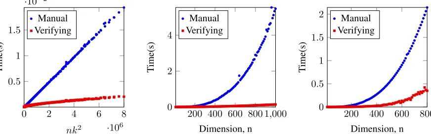
Figure 1: Experimental Results, with time taken for self computation (blue dots), and for verification (red squares).
the scatter matrices, with this we then use the method in Section 3.6 to find Vˆ and Dˆ with error . This is a
d2log(qd/),log(qd/)-protocol, note however that we
are only interested in columns ofVˆ corresponding to
non-zero eigenvalues. We can use these get our r ≤ k−1
vectors to form W and computeWTS using the matrix multiplication protocol to get the desired result. Our to-tal protocol will therefore be(dnlog(nqd/),log(nqd/))
from constructing our scatter matrices.
5 Practical Results
We performed a series of experiments with a field size of q = 231 − 1, using implementations in C of our
protocols for matrix multiplication, inversion, and eigen-decomposition. We used a machine with an Intel i7 processor and 16 GB of memory. We worked on matrices up to 1000 by 1000, as this allowed us to get a distinguish-ing result between the verifier runndistinguish-ing the computation and the verifier using our checking protocols. We used the GNU Scientfic Library for C, using gsl blas dgemm for matrix multiplication, gsl linalg LU invert to find the inverse andgsl eigen symm for the eigen-decomposition. The verification was done on the result produced by the self-computation. We created dense random matrices with entries drawn uniformly. Note that our protocols do not depend on any structure in the matrices, so uniform random data suffices to test them. Where we require symmetric matrices, we setAij =Aji∀i < j.
Our verification protocols were built as discussed in the paper, with the time taken to find the fingerprints of all relevant matrices and check the necessary bounds being the verification time seen in Figure 1. We tested the veri-fication protocols against a variety of incorrect matrices, which were successfully rejected. The memory costs for our verification, even in the case ofA ∈ F1000×1000
q was
only a few hundred bytes, a significant reduction over self computation, which would be in the order of several megabytes. The communication cost is the cost of sending the matrix, simply the size of the matrix multiplied by a small constant. Consequently, the main aim of our experiments is to quantify the potential timing gains of verification over self-computation.
For our matrix multiplication protocol (Figure 1a), we con-sider the number of scalar multiplications required to find the result of multiplyingA∈Fk×n
q andB∈Fnq×k, that is,
k2n. When we plot the time taken againstk2n, we see the
expected linear relationship between self-computation and time taken. The verifier needs to compute the fingerprint of A,B, which will involvenkmultiplications, and AB, which involves k2 multiplications. This agrees with the
observation in the graph; that the self-computation time is linear, and the verification time is sublinear.
In both matrix inversion (Figure 1b) and eigen-decomposition (Figure 1c), we see the expected cubic increases in running time for self-computation, with a significantly lower increase for the verification. The verification running time depends primarily on theO(n2)
cost of computing the needed fingerprints, as above, and as such, we see the asymptotically shallower lower curve.
6 Concluding Remarks
We have introduced effective protocols for checking mod-els generated by common tasks, such as Ordinary Least Squares, Principal Components Analysis and Linear Dis-criminant Analysis. Natural next steps are to study more complex models, such as Support Vector Machines, and (initially shallow but ultimately deep) neural networks, which have high training costs but could be cheap to verify.
References
L´aszl´o Babai. Trading group theory for randomness. In
Proceedings of the seventeenth annual ACM symposium on Theory of computing, pages 421–429. ACM, 1985. Amit Chakrabarti, Graham Cormode, and Andrew
Mcgre-gor. Annotations in data streams. Automata, Languages and Programming, pages 222–234, 2009.
Graham Cormode, Justin Thaler, and Ke Yi. Verifying computations with streaming interactive proofs. Pro-ceedings of the VLDB Endowment, 5(1):25–36, 2011. Graham Cormode, Michael Mitzenmacher, and Justin
Thaler. Practical verified computation with streaming interactive proofs. InProceedings of the 3rd Innovations in Theoretical Computer Science Conference, pages 90– 112. ACM, 2012.
Graham Cormode, Michael Mitzenmacher, and Justin Thaler. Streaming graph computations with a helpful ad-visor.Algorithmica, 65(2):409–442, 2013.
Samira Daruki, Justin Thaler, and Suresh Venkatasubra-manian. Streaming verification in data analysis. In In-ternational Symposium on Algorithms and Computation, pages 715–726. Springer, 2015.
Pierre A Devijver and Josef Kittler. Pattern recognition: A statistical approach. Prentice hall, 1982.
R¯usin¸ˇs Freivalds. Fast probabilistic algorithms. Mathe-matical Foundations of Computer Science 1979, pages 57–69, 1979.
Shafi Goldwasser and Michael Sipser. Private coins versus public coins in interactive proof systems. InProceedings of the eighteenth annual ACM symposium on Theory of computing, pages 59–68. ACM, 1986.
Shafi Goldwasser, Yael Tauman Kalai, and Guy N Roth-blum. Delegating computation: interactive proofs for muggles. In Proceedings of the fortieth annual ACM symposium on Theory of computing, pages 113–122. ACM, 2008.
Johan H˚astad and Avi Wigderson. The randomized com-munication complexity of set disjointness. Theory of Computing, 3(1):211–219, 2007.
This will cover the proofs required for checking eigenvalues of a symmetric ma-trix, checking the symmetric generalised eigenvalue problem and the protocol for fingerprinting the covariance matrix.
1.1
Details of Theorem 3
We use the fact thatλi ≤ kAk2, andkvik2 = 1. We also have krk2≤
√
n
2 and
|ρ| ≤ 1
2, and so;
kT Avbi−λbivbik∞≤√nkT Avbi−λbivbik2
=√nkT2Av
i+T Ar−T2λivi−T ρvi−T λir−ρrk2
≤√n(TkAk2krk2+T|ρ|kvik2+T|λi|krk2+|ρ|krk2)
≤T nkAkF +T √n
2 +
n
4
kvbiTvbj−T2δijk∞≤√nkvbiTvbj−T2δijk2
≤√nk(T vi+r)T(T vj+r)−T2δijk2
≤√nkT viTr+T rTvj+rTrk2
≤2T√nkrk2+√nkrk22
≤T n+n
√n
4
1.2
Details of Theorem 4
First definevei =viTb,λei=λiTb, so we have;
kT Avbi−λbivbik∞
T2 =kAvei−λeiveik∞≥
kAvei−λeiveik2
√n
As A is symmetric, we can writeA=V DVT, whereV is the orthogonal matrix
of eigenvectors, andDis the diagonal matrix of corresponding eigenvalues. Then
kAvei−λeiveik2=kV DVTvei−λeiveik2
=kV(D−λei)VTveik2
=k(D−λei)VTveik2
≥min
j (|λj−λei|)kV T
e
vik2
= min
j (|λj−λei|)kveik2
≥min
j (|λj−λei|) r
1−
√n
T − n
4T2
= min
j (|λj−λei|) r
1−1 2 −
1 16 if
√
n≤ T
2
≥minj(|λ2j−λei|)
So if we consider >0, and wish to ensure that minj(|λj−λei|)< , i.e. there
is a (true) eigenvalue close to the approximate eigenvalue, then we can choose aT based on
min
j (|λj−λei|)≤2kAvei−λeiveik2 ≤2√nkAvei−λeiveik∞
≤ 2 √n
kT Avbi−λbivbik∞
T2
≤ 2n √n
kAkF
T +
n T +
n√n
2T2 (using Theorem 3)
AsT tends to infinity, this bound positively approaches 0, as such, for any >0 we can find aT s.t. the error inRof minj(|λj−λei|) will be.
1.3
Details of Theorem 8
The Cholesky Decomposition allows us to solve the symmetric generalised eigen-value problem forA, B ∈Fn×n
q , with A symmetric, andB symmetric positive
semi-definite;
FindV, D∈Rn×n such thatAV =BV D
We do this by finding the Cholesky Decomposition ofB,L and then perform-ing findperform-ing the eigenvalues of the symmetric matrix C =L−1A(L−1)T to get
matricesV0, D0 with CV0 =V0D0. D =D0, andV =L−1V0 are the solutions we desire.
With our approximations, we use our matrix inversion and Cholesky Decom-position protocols to find, using scaling factor T1, we have that ˆC will be in
ˆ
C=( ˆ\L)−1A( ˆ\L)−1
So we have
ˆ
LLˆT =T12B+E1 E1∈
−nk2BT1kF,nkBkF
2
n×n
ˆ
L( ˆ\L)−1=T1I+E2 E2∈
−nkBˆkF−n
2
4 , nkBˆkF+
n2
4
n×n
If we receive approximate eigenpairs, ˆU ,Dˆ with diagonal ˆλ, of ˆCfrom the helper, with scaling factorT giving errorδ, satisfying
kTCˆUb−DbUbkmax≤
T nkCkF+
T√n
2 +
n
4
kUbTUb−T2Ikmax≤
l
T√n+n 4
m
LetDδ, Uδ
∈Rn×n be the true eigenvalues and eigenvectors of ˆC. So
ˆ
CUδ =UδDδ
We know thatkT Dδ
−Dˆkmaxwill be at mostT δ. Furthermore let ˆLTVδ =Uδ,
so
ˆ
CUδ=UδDδ \
( ˆL)−1A( ˆ\L)−1
T
ˆ
LTVδ= ˆLTVδDδ
ˆ
L( ˆ\L)−1A( ˆ\L)−1
T
ˆ
LTVδ= ˆLLˆTVδDδ
(T1I+E2)A(T1I+E2)TVδ= (T12B+E1)VδDδ
A+E2A+AE
T
2 +E2ET2 T2
1
T
Vδ=
B+E2
T2 1
VδDδ
By using the eigenvalue perturbation theory [?], we can say that there exists
V ∈Rn×n,D
∈Rn×n with diagonalλ, so
λi=λδi +vδi
TE2A+AE2T +E2ET2
T2
1 −
λδi
E1 T2 1
viδ
|λi−λδi|=|viδ
T E2A+AE2 +E2E2
T2 1 − λδ i E1 T2 1 vδ i|
≤vδi T 2
E2A+AET
2 +E2ET2 T2
1 −
λδi
E1 T2 1 2 vδi
2 ≤
E2A+AE T
2 +E2E2T −λδiE1
T2 1 2
≤ kE2Ak2+ AET
2
2+E2ET
2
2+λδ
iE1 2
T2 1
≤ 2kE2k2kAk2+kE2k
2
2+kCˆk2kE1k2 T2
1
≤
2nnkBk2+n
2
4
kAk2+n2
nkBk2+n
2
4
2
+kCˆk2nnkBk2
2 T2 1 ≤
2n2
kBk2+n
3
2
kAk2+
n4
kBk2
F+k Bk2n5
2 +
n6
16
+kCˆk2n2kBk2
2 T2 1 ≤
2n2
kBˆk2+n
3
2
kAk2+
n4
kBˆk2
2+kBk2n
5
2 +
n6
16
+kCˆk2n2kBk2
2
T2 1
≤ 32n
2
kBk2kAk2+ 8n3kAk2+ 16n4kBk22+ 8kBkFn5+n6+ 8kCˆk2n2kBk2 T2
1
As,A, B∈Fq, we havekAk2,kBk2≤qn,kCˆk2≤qnT1
|λi−λδi| ≤
32n2(nq)2+ 8n3nq+ 16n4(nq)2+ 8nqn5+n6+ 8qnT1n2nq T2
1
≤ 32n
4q2+ 8n4q+ 16n6q2+ 8n6q+n6+ 8qnT1n3q T2
1
≤ 8n
4(4q2+q) +n6(16q2+ 8q+ 1) + 8qnT1n3q T2
1
≤ q
3n4 T1
If we have thatq≥20,n≥3 andT1≥n2. We also have
|T λδi −λˆi| ≤T δ
So
|T λi−λˆi| ≤ |T λi−T λδi|+|T λδi −λˆi|
≤T
q3n4 T1 +
δ
|T λi−λˆi|
T ≤
q3n4 T1 +
δ
Therefore, to get the generalised eigenvalues to an error of we must choose
T, T1 such that
T= q
2n5 2
δ ≥
qn32kCˆk
δ
T1= q
3n4 −δ
Whereδ < .
If we takeδ =
2, then we have
T =2q
2n5 2
T1=2q
3n4
And our total protocol is therefore, assumingq > n, n2log q3n4/,log q3n4/.
1.4
Fingerprinting the Covariance Matrix
Algorithm 1:Streaming AnnotatedCovarianceFingerprint
Input :S∈Fd×n
q
Output:fx(A) =fx (n−1)Cov(S)or⊥
1 Choosex∈RF
2 Whilst StreamingS column by column;
3 forSj↓ with j= 0to n−1 do
4 Construct the sum of each of thesefxvn(Sj↓),fxv(Sj↓),fxvn(Sj↓)fxv(S↓j), Pd−1
i=0 Sijxn and
Pd−1
i=0 Sijxni individually
5 fx(A) =Pjfxvn(Sj↓)fxv(Sj↓)− hP
j Pd−1
i=0 Sijxni hPjfxvn(S↓j) i
− hP
j Pd−1
i=0 Sijxni
i hP
jfxv(Sj↓) i
+nhPjPdi=0−1Sijxni hPjPdi=0−1Sijxni i
6 ReceiveAbfrom the helper
7 Check
8 fx(A) ==fx(Ab)
This algorithm provides a d2log(qn),log(qn)
−protocol for verification thatA
is indeed the covariance matrix scaled byn. The costs come from scaling byn
and receivingA∈Fd×d qn .