Accepted Manuscript
The non-persistent relationship between foreign equity flows and emerging stock market returns across quantiles
Cheng Yan, Xichen Wang
PII: S1042-4431(17)30539-5
DOI: https://doi.org/10.1016/j.intfin.2018.03.002 Reference: INTFIN 1033
To appear in: Journal of International Financial Markets, Institu-tions & Money
Received Date: 12 November 2017 Accepted Date: 17 March 2018
Please cite this article as: C. Yan, X. Wang, The non-persistent relationship between foreign equity flows and emerging stock market returns across quantiles, Journal of International Financial Markets, Institutions & Money (2018), doi: https://doi.org/10.1016/j.intfin.2018.03.002
1
The non-persistent relationship between foreign equity flows
and emerging stock market returns across quantiles*
Cheng Yan
a, Xichen Wang
ba Durham University Business School; b Lancaster University Management School
February 25, 2018
ABSTRACT
We compare the performance of two state-of-the-art predictive regression methods of IVX-Wald (Kostakis et al., 2015), IVX-Quantile regression (Lee, 2016) with the traditional OLS in examining the relationship between foreign equity flows and emerging stock market returns. By doing so, we take into account not only the potential persistence in foreign equity flows, but also the exceptional behavior of the extreme foreign flow episodes. We find a robust positive relationship between equity flows and contemporaneous stock returns among emerging stock markets (especially in Asia), but little evidence for intertemporal return predictability.
Keywords: Emerging stock markets; International Capital Flows; Predictive regression; IVX filtering.
JEL classification: C22, G12, G15
*
2
The non-persistent relationship between foreign equity flows
and emerging stock market returns across quantiles
ABSTRACT
We compare the performance of two state-of-the-art predictive regression methods of IVX-Wald (Kostakis et al., 2015), IVX-Quantile regression (Lee, 2016) with the traditional OLS in examining the relationship between foreign equity flows and emerging stock market returns. By doing so, we take into account not only the potential persistence in foreign equity flows, but also the exceptional behavior of the extreme foreign flow episodes. We find a robust positive relationship between equity flows and contemporaneous stock returns among emerging stock markets (especially in Asia), but little evidence for intertemporal return predictability.
Keywords: Emerging stock markets; International Capital Flows; Predictive regression; IVX filtering.
3
1. Introduction
How do foreign investors affect the stock movements in Emerging Markets Economies
(EMEs)? This is a question of essential importance for both researchers and policymakers, as well as a long-standing debate in International Economics/Finance. The growing cross-border capital flows represent the most prominent form of global financial integration, the degree of which has noticeably increased over the past decades. In particular, global capital flows increased from 7% of the world GDP in 1998 to over 20% in 2007, but suffered large reversals in late 2008 and re-surged after that (Milesi-Ferretti and Tille, 2011). At the same time, stock prices in EMEs went up sharply in 2007, but dropped even more than developed markets in 2008, and recovered faster than the developed markets (Bartram and Bodnar, 2009; Yan et al., 2016). Due to this seemly coincidence, it is not uncommon to conjecture two hypotheses: 1) the sizable foreign flows have caused the stock movements in EMEs, i.e., price pressures1; 2) foreign investors can predict the stock movements in EMEs (Ahmed and Zlate, 2014).
Both hypotheses are plausible and rooted in the literature. On the one hand, the literature has documented a positive contemporaneous relationship between equity flows and returns2. On the other hand, it has been conjectured that one major motive for foreign investors is return-chasing (i.e., chase higher future returns), and higher returns in the future will attract more equity flows3. If this motive is true, foreign investors must have the ability to predict future stock movements in the first place.
The literature typically use OLS based methods such as vector autoregressive models to test the first hypothesis4, while the second hypothesis has rarely been tested, probably because that the classic method (i.e., predictive regressions) for return predictability research
1
See, for example, Tong and Wei (2011), Jotikasthira et al. (2012), Yan et al. (2016), Puy (2016), Fuertes et al. (2017).
2See, e.g., Brennan and Cao (1997), Griffin et al. (2004), Richards (2005), Hau and Rey (2004, 2006). Ülkü and Weber
(2014), Ülkü (2015), Yan et al. (2016), Fuertes et al. (2017). Richards (2005) offers a simple story based on demand shocks to illustrate the mechanism: holding the portfolio preferences of domestic investors unchanged, decisions by foreigner investors to buy (sell) are demand shocks leading to an outward (inward) shift of aggregate demand curve and thereby an increase (a decrease) of stock prices. The market microstructure literature further paves the theoretical foundation for this hypothesis.
3
See, for example, Bohn and Tesar (1996), Brennan and Cao (1997), Raddatz and Schmukler (2012), Curcuru et al. (2011, 2014), Fuertes et al. (2017). The return-chasing hypothesis has been embedded in various theoretical models (Brennan and Cao, 1997; Albuquerque et al., 2007, 2009; Dumas et al., 2017).
4
4
does not suit foreign flows due to their potential persistence. It would be serious to neglect equity flows’ persistence5
because it will give rise to invalid results if equity flows are employed as a predictor in a standard predictive regression. In particular, Campbell and Yogo (2006) show that if the predictor is strongly persistent, empirical results based on standard regression models such as OLS will suffer severe size distortion leading to an over-rejection of the null hypothesis of no predictability. Since it is difficult to identify the exact degree of persistence precisely, standard unit root tests hardly provide a firm guide (Lee, 2016). To tackle this potential problem, we employ the predictive regression model based on IVX-filtering (Kostakis et al., 2015), which can handle predictor variables with various degrees of persistence.
On the other hand, the traditional OLS based methods have been criticised recently as well. Using a quantile regression model, Ghosh et al. (2014) demonstrate that international flows behave differently during normal periods and extreme episodes such as surges, stops, flight, and retrenchment6. To tackle this potential problem, we employ the IVX-version of quantile regression (IVXQR) of Lee (2016), which enables us to examine the predictability of stock returns across all quantiles of its conditional distribution. Both the predictive regression model with IVX-filtering and the IVX-version of quantile regression are sophisticated and flexible models, which are used for the first time in a study of international capital flows and constitutes our methodical contribution in this paper. More importantly, these two models allow us to provide a comprehensive and robust answer to the initial question of how foreign investors affect the stock movements in EMEs by ensuring that the results would not be a statistical artifact because of the persistent predictor.
We choose to focus on portfolio equity flows in this paper, as it is straightforward to conjecture that stock bubbles in EMEs were more likely to be associated with portfolio equity flows, than other types of short-term flows such as portfolio bond flows and bank flows.
5
This persistence of capital flows is grounded in the literature. Albuquerque et al. (2007) develop a theoretical model predicting persistence as an enduring feature of foreign investors’ trading, because of the heterogeneity within their group of accessing and responding to new information. In addition, foreign investors may divide their trading into small parts to reduce their trading costs brought by price pressures (Kyle, 1985). Accordingly, Froot et al. (2001) Griffin et al., (2004), Richards, (2005), Ülkü and Weber (2014), Ülkü (2015), and Fuertes et al. (2017) found empirical evidence that capital flows are auto-correlated. Although it is difficult to identify the exact degree of persistence precisely, Sarno and Taylor (1999a, b) and Fuertes et al., (2016) have identified both a persistent and a temporary component in various kinds of international capital flows.
6
5
Moreover, portfolio equity flows are easy to access at relatively high frequencies (at least monthly), which may not be so easy to access for other types of short-term flows such as bank flows, which are usually available at quarterly frequency (Fuertes et al., 2016). We exclude long-term capital flows such as Foreign Direct Investment (FDI) and official flows as they differ from short-term capital flows in nature (e.g., Tong and Wei, 2011; Fuertes et al., 2016). Short-term flows are more volatile and speculative, and they could rush into a country and then run out precipitously because of return-chasing. Therefore, short-term speculative capital flows are more likely to affect local financial markets than long-term flows.
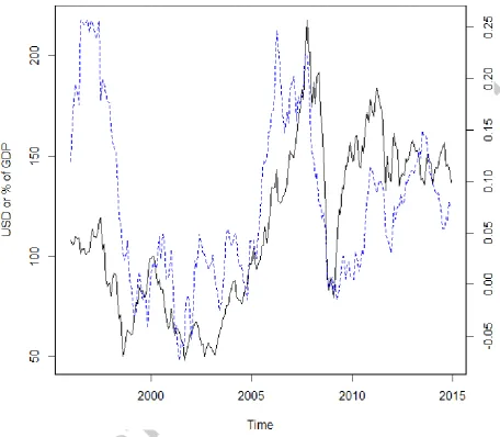
To conduct our empirical analysis, we collect monthly data for 21 EMEs over 1995-20147. Our data for stock prices are collected from Morgan Stanley Capital International (MSCI), and data for equity flows are from Treasury International Capital (TIC). Figure 1 plots the data of both average equity flows and stock prices of all the EMEs in our sample to enable us to have a glimpse of the correlation between these two variables. The solid black line represents an overall MSCI stock price index of the EMEs, while the dashed blue line shows the average equity flows towards all EMEs in our database, scaled by domestic GDP.
[Insert figure 1 around here]
Figure 1 seems to suggest a co-movement and a lead-lag relationship between these two variables, and this pattern becomes more evident after the early 2000s, after which the global financial market had been significantly integrated. Specifically, both equity flows (lead) and stock prices (lag) rose before the millennium, around which the dot.com bubble was present in the U.S. stock market. As this “information technology bubble” collapsed in
the early 2000s, both equity flows and stock prices in EMEs dropped, reaching the bottom around late 2001. Nevertheless, a more noticeable pattern of co-movements appeared in the mid-2000s: both equity flows and stock prices surged until the outset of the global financial crisis. However, after 2008, both time series collapsed sharply and semi-simultaneously. One might observe from Figure 1 that this drop is more sizable and prolonged than any other. Finally, in the post-crisis era, equity flows and prices appear to co-move again. In sum, we observe several patterns of co-movements and a lead-lag relationship between equity flows and stock prices, which motivates our further analysis.
7
6
Our main findings can be summarized as follows. We first investigate the link between equity flows and contemporaneous returns. We start with OLS and find a significant association between these two variables among a large number of EMEs, especially among the Asian stock markets. The estimated coefficients of equity flows are mostly positive. To rule out the potential size distortion resulted from equity flows’ persistence, we employ the
latest IVX models. Based on the predictive mean regression of Kostakis et al. (2015), we confirm that our results are not a statistical artifact owing to a persistent regressor. Based on the IVX-version of quantile regression of Lee (2016), we also show that equity flows are generally significant across a wide range of quantiles.
Secondly, we investigate the association between equity flows and one-month-ahead stock returns, in which practitioners might be more interested. We find little evidence for the stock return predictability of foreign investors in EMEs. Only a few countries, namely Poland and South Africa, show strongly significant estimates. The disappearance of equity flows’
significance is in line with the findings of Richards (2005), which finds a significant price impact associated with foreigners’ trading on six Asian EMEs. However, this price pressure typically disappears within days. Similarly, in our study, it is likely that equity flows’ price
impact is short-term so that they contain limited information to predict one-month-ahead returns. In addition, equity flows’ estimated signs are usually negative8.
Finally, we also conduct an out-of-sample analysis, and find that only equity flows in Poland can outperform the benchmark model. In summary, this study finds a significant contemporaneous association between equity flows and international equity flows. Although the monthly equity flows appear to contain limited (if any) information to forecast one-month-ahead stock returns in EMEs, our empirical tools could be a fascinating venue for future research using equity flows’ data of higher frequency (such as weekly or even daily), whose persistence could be significantly stronger (e.g., Ülkü and Weber, 2014; Ülkü, 2015).
The remainder of this paper is organized as follows. Section 2 discusses our empirical methodology, and Section 3 describes our data set as well as summary statistics. Section 4 presents our empirical results. Section 5 concludes. Section 6 is the appendix section, which discusses our filtering approach, and gives a brief description of recent predictive regressions models based on IVX-filtering.
8
7
2. Model estimations based on IVX
This section presents two unbiased approaches to tackle the potential persistence of capital
flows: The mean regression with IVX-Wald test proposed by Kostakis et al., (2015), and the
Quantile regression IVX-QR approach proposed by Lee (2016).
2.1. Mean regression: IVX-Wald (Kostakis et al., 2015)
For the conditional mean regression of stock return predictability, we use the model proposed by Kostakis et al. (2015). Denote all the demeaned variable as: , , and , and then the resulting demeaned regression matrices would be:
and . Similarly, we denote the (undemeaned) instrument matrix
as . Then it is convenient to rewrite the model in Equation (A.1) as follows:
. (1)
The IVX estimation of A from the predictive regression (1) is analogous to a two-stage-least-squares estimator based on the instrument with (MI) persistence in (A.4). Formally, it is:
. (2)
Kostakis et al. (2015) further show that IVX-estimators are asymptotically mixed normal, and the linear restrictions on the coefficient matrix A from (A.1) or (1) could be tested by a standard Walt test, which is easier than earlier models based on the Bonferroni method.
2.2. Quantile regression IVX-QR (Lee, 2016)
While most of the literature focuses on predicting the conditional mean of stock returns, it is interesting to investigate the predictability at each quantile across the whole conditional distribution of returns9. Firstly, financial data are typically known as having heavy tails and skewed distributions. Such features might imply potentially greater predictability at certain quantiles rather than only the median (Lee, 2016). Secondly, in many areas of financial economics, it might be even more interesting to examine the entire return distribution or specific parts of the distribution such as tails. For instance, risk managers may pay more
9
8
attention to the left tail. Thirdly, the literature reports that equity flows could be pro-cyclical, which implies that equity flows might have a more substantial impact on some particular quantiles (such as the two tails). For example, Broner et al. (2006) find that international mutual funds tend to increase (decrease) their weights of countries in which they have a large (small) portfolio weights when the funds are doing relatively well (poorly). Raddatz and Schmukler (2012) also find that both individual investors and fund managers tend to take too much risk during good times. However, they would run and retrench quickly when shocks hit the financial system. Therefore, it is interesting to examine whether equity flows exhibit a more significant predictability conditional on turbulent episodes—two tails of returns distribution. To that end, the application of Quantile Regression (QR) in Koenker and Basset (1978) has some merits.
However, QR faces the same problem of non-standard distortion as the mean regression does if the regressor is highly persistent. To solve this problem, Lee (2016) adopts the same IVX instrumentation (Philllips and Magdalinos, 2009) and develops the IVX-quantile regression (IVX-QR) allowing for persistent predictors. To formalize this model, let us first consider a linear predictive QR model:
, (3)
where is a conditional quantile of the dependent variable (stock returns). Then
the ordinary QR estimator has the form:
, (4)
where is the asymmetric QR loss function and u
is QR the residual.
The IVX-QR estimation starts with a de-quantile procedure, which is analogous to the demeaning process in the mean regression. Formally, we remove the intercept term in (3):
, (5)
where . Based on the IVX-instrument from Equation (A.5), the IVX-QR estimator is:
9
where . Lee (2016) shows that the resulting test statistics follows a chi-square limit distribution, which is empirically easy to compute.
3. Data and descriptive statistics
Our dataset covers 21 EMEs from January 1995 to December 2014. We start with January
1995 because some countries’ data (e.g., Czech and Hungary) are not available before this
time. We end our sample at December 2014, one year earlier than the time of writing (i.e.,
January 2016), to alleviate the potential data revisions to equity flows and aggregate prices10.
We divide these countries into four groups according to their regions. The first group consists
of seven countries from Asia: China, India, Indonesia, Malaysia, Pakistan, Philippines, and
Thailand. The second group includes six Latin American countries: Argentina, Brazil, Chile,
Colombia, Mexico, and Peru. The third group contains four EMEs from emerging Europe:
Czech, Hungary, Poland, and Russia. Finally, we classify the remaining countries in our
sample into one group: Egypt, Morocco, Turkey and South Africa.
The stock returns, defined as logarithmic monthly changes in dividend-adjusted MSCI
global stock indices in U.S. Dollars (USD) 11, are collected via Bloomberg. We compute
excess returns as the difference between monthly stock returns and the one-month Treasury
bill rate.
We obtain monthly international equity flows from the U.S. to the 21 EMEs. We collect
the data from the Treasury International Capital (TIC) database of the U.S. Treasury
Department, following the extant literature (e.g., Sarno et al., 2016; Fuertes et al., 2016).
We use gross flows rather than net flows to avoid possible contamination from the
behavior of domestic investors (Rothenberg and Warnock, 2011; Forbes and Warnock, 2012).
10
Ideally, we should use all the observations available if all variables can be observed contemporaneously without any revisions. Unfortunately, this is not the case in reality. Specifically, all equity flows and CPI indices are known with lags and are subject to revisions over time. In other words, stock indices are known in real time but equity flows and aggregate prices are not. Therefore, in reality the two sets of data are not observed contemporaneously. We are not aware of a better way to deal with this problem and most of the extant studies suffers from it as well. We thank a referee for pointing it out.
11
10
As the extant literature mostly discusses the impact of foreign investors who are domiciled in
developed markets but invest in the stock markets of EMEs (e.g., Broner et al., 2006 and
Jotikasthira et al., 2012), we focus on gross inflows, defined as the net of U.S. purchases of
domestic stocks and U.S. sale of domestic assets (Forbes and Warnock, 2012). Therefore, a
positive entry indicates an inflow into an EME from the U.S. Finally, all flows are in millions
of USD, and we deflate each time series by U.S. CPI to convert it into real values.
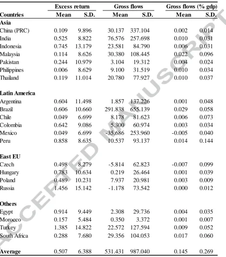
[Insert Table 1 around here]
Table 1 reports the descriptive statistics. Excess returns average about 0.506% across
countries, and their standard deviations are on average 9.81%, indicating the high stock
volatility in EMEs. As for flows, they average about 25.306 million USD and 0.006 % of
nominal GDP across countries, and their high standard deviations reveal equity flow’s
volatile nature. Across 21 EMEs, average standard deviations are 126.067 million USD
(when flows are measured in USD) and 0.046 % (when scaled by domestic GDP). We do not
report the traditional Unit root test results, as Lee (2016) points out that “Unit root tests do
not provide a firm guidance on the discrepancy between I(0), near or exact unit root
processes.”
4. Empirical results
To assess the predictability of stock returns from international equity flows, we present our
empirical results in two parts. In the first part, we report our results of in-sample tests. In the
second part, we show the out-of-sample tests’ results.
4.1. In-sample tests
In this sub-section, we first investigate the contemporaneous relationship and after that move
to the lead-lag relationship between current flows and one-month-ahead returns.
4.1.1 Contemporaneous returns
11
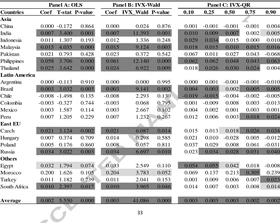
flows and stock returns. Panel A of Table 2 reports our results based on OLS, which suggests
that equity flows significantly affect stock returns contemporaneously: 9 out of 21 EMEs
display significant estimates at 10% level, and among them 8 are significant at 5% level. For
these 9 EMEs, their estimated coefficients are all positive. Taking India for example, if equity
flows increases by 100 Million USD (in real value), its domestic stock return is likely to
increase by 0.7%. This positive sign is consistent with the price pressure stories arguing that
the equity flows rush into an EME could drive up stock prices quickly (e.g., Richards, 2005).
Panel A of Table 2 suggests that equity flows have a heterogeneous impact among
different regions. Specifically, the Asian countries are more severely affected. Among the 7
Asian EMEs in our sample, 4 (India, Malaysia, Philippines, and Thailand) display a
significant slope estimate of equity flows. As for the other 14 EMEs, we also observe
significant estimates from Brazil, Czech, Russia, Egypt and South Africa. However, these
countries are spread across different regions (Latin America, East Europe, and others), and no
other region contains such a considerable percentage of significant estimates as Asia does. A
number of empirical studies—e.g., Richards (2005) and Tillman (2013)—also support the
observation that Asian equity flows significantly affect the local stock prices. Nevertheless,
few theoretical studies clarifies why this observation is particularly significant in Asia
compared to other regions.
[Insert Table 2 around here]
If equity flows are persistent or belong to the I (1) space, empirical results based on OLS
would be invalid. Worse, it is also empirically challenging to identify the exact degree of
persistence, which also confuses the validity of OLS estimates. Therefore, Panel B of Table 2
reports our results based on IVX-filtering predictive regression of Kostakis et al. (2015),
which remains valid when handling predictors with various degrees of persistence.
12
of Table 2. Again, 9 (8) out of 21 EMEs show significant coefficient at 10% (5%) level. The
geographical pattern stays similar. Asian countries remain the most significant group that
displays significant estimates. This similarity suggests that the significant estimates of equity
flows are not statistical artifacts due to the predictors’ persistence. Therefore, our results
(based on IVX-filtering technology) confirm the significant association between international
Equity flows and contemporaneous stock returns in EMEs.
IVX-QR
Our empirical results based on predictive mean regression can be informative. However,
given our previous discussion of equity flows’ pro-cyclical nature, we also examine the entire
return distribution or specific parts of the distribution such as tails and center.
Asian
Panel C of Table 2 presents our empirical results from the 10th to the 90th quantile based
on IVXQR. One can still observe that the equity flows’ effect on stock returns is the strongest
among the Asian EMEs. Out of the 7 Asian countries in our samples, the 4 EMEs (India,
Malaysia, Philippines, and Thailand) where equity flows are significant in the conditional
mean regression all display significant results across a wide range of quintiles. Equity flows
in India appear significant through the returns’ conditional distribution except for the 75th
quantile. The magnitude of their estimated coefficient varies from 0.005 to 0.010, and it is
slighter more substantial in the left tails (10th to 50th). Indian equity inflows have a more
significant price impact conditional on episodes of relatively low returns. Equity flows into
Thailand have positive and significant coefficients from the 25th to the 75th quantile.
Moreover, we observe a more pervasive effect from Malaysia and Philippines: equity flows
towards these two countries possess positive and significant coefficient estimates across all
quintiles reported (10th to 90th).
13
distribution, which has been overlooked by the conditional mean regression. For instance,
equity flows to Indonesia lack significance in both of the conditional mean regressions, as
shown in Panel A and B of Table 2. Nevertheless, our results based on IVXQR (in Panel C of
Table 2) report positive and strongly significant coefficients in the left tail (from 10th to 25th).
Indonesian equity inflows eventually become insignificant in the upper quantiles. This
finding based on quantile regression suggests a heterogeneous effect across different parts of
returns’ distribution, and thereby imply that the price impact of equity inflows into Indonesia
might be more substantial when returns are relatively lower. As international investors retreat
from the local stock markets quickly during bad times (e.g., Raddatz and Schmukler, 2012),
the heterogeneous price effect found in this study could be in line with this pro-cyclical
nature.
Latin America
Table 2 also shows that equity flows into Latin America have a considerably smaller
impact on returns, than the ones into Asia. Among the 6 Latin American EMEs, only equity
flows to Brazil are significant across the whole conditional distribution. Moreover, those
coefficients are all positive. This observation is once again in line with theory, as we
previously discussed in Section 1. As for some other Latin American countries, equity flows
appear with significant estimates in a few quantiles in one tail of returns’ distribution. For
example, equity flows to Chile are significant in the 10th and the 25th quantiles, which
suggests that equity flows have a stronger contemptuous predictability of returns when
returns are relatively low. However, the pattern in Peru is completely the opposite: equity
flows are only significant when returns are relatively high ( ). For these
two countries, equity flows’ price impact is significant only at the two tails of returns’
conditional distribution, which again implies that equity flows might have a stronger impact
14 East Europe
Turning to the East European countries, Equity flows to the Czech Republic and Russia
are still significant across a considerable amount of quantiles. These observations are
consistent with the results from the conditional mean regressions (shown in Table 2). In
particular, equity flows to Russia are significant across the whole distribution: they possess
positive and statistically significant coefficients from the 25th to the 90th quantile. However,
equity flows’ price impact is asymmetric in Czech, as we only observe significant estimates
in the right part of the returns’ conditional distribution implying episodes when the stock
returns are booming.
Others
The bottom panel of Table 2 shows the results for the other EMES: mainly countries
from the Middle East and Africa. Firstly, equity flows to Egypt and Morocco are insignificant
in the conditional mean regressions (as shown in Panel A and Panel B of Table 2). However,
our results based on IVXQR suggest that equity flows to these two EMEs might possess more
predictability in some specific parts of the distribution. Starting with Egypt, equity inflow has
a positive effect on returns conditional on episodes when returns are low (at lower quantiles),
but this effect decreases and becomes insignificant after the 50th quantile. For Morocco,
Turkey, and South Arica, equity flows’ effect (on returns’ predictability) is not significant at
the left tail but the right tail of the conditional distribution. For instance, at the 75th percentile,
a 10 million USD increase of equity flows to Morocco would be associated with a 3.0%
increase in returns. This implies a significant price impact of equity flows to Morocco, which
is a relatively small economy compared to the other EMEs in our sample. Overall, for these
EMEs, quantile regression suggests more predictability in the two tails.
In summary, our results suggest that equity flows towards Asian countries significantly
15
Pakistan display no significant coefficient in any quantile reported. Furthermore, compared to
the outcomes from the previous two conditional-mean regressions, our results based on
IVX-QR show two additional implications: first, for some countries (especially those in Asia),
equity flows affect equity prices during both booms and busts (throughout the whole
conditional distribution of returns). Second, for a few other countries, predictability is only
found during episodes of either expansion or contradiction. For instance, predictability in the
Egyptian stock markets is only found in returns’ lower quantiles; this shows the association
between flows and returns only exists when returns are relatively low. Likewise, we could
only observe stock return predictability in Peru and Czech during good times—that is, the
upper quantiles.
4.1.2 One-month-ahead returns
Our results on the contemporaneous relationship may not be enough for the practitioners,
who are more interested in whether international equity flows can predict future stock returns.
To that end, we report the results of one-month-ahead predictability based on the same set of
empirical models (OLS, IVX-Wald, and IVXQR) used previously. We start with OLS
estimates.
OLS
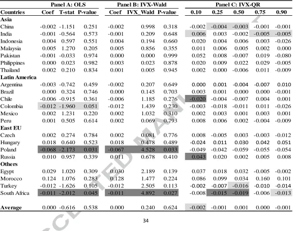
The Panel A of Table 3 shows the one-month-ahead results based on OLS. One might
observe several striking findings: firstly, the predictability mostly disappears. This is most
prominent in Asian markets, that equity flows lack significance in all of the seven Asian
EMEs. This observation is a sharp contrast to our results reported in Table 2, where
contemporaneous equity flows display significantly positive estimates in four out of seven
Asian markets. This is probably due to the short-term nature of equity flows’ price impact.
Richards (2005) uses daily data to investigate the link between net purchases of foreigners
16
beyond the day of inflow, but most of this impact is complete within a few days. This finding
might help to explain our empirical results here: when international equity inflows enter the
domestic stock markets, they drive up stock returns contemporaneously, but their impact
might perish within days. Therefore, there is no significant link between equity flows and
one-month-ahead returns.
Another somewhat surprising observation is that among the countries where equity flows
are significant (Colombia, Poland, and South Africa), the estimated coefficients for equity
flows are all negative. Take Poland for instance: if foreign equity inflow goes up by 10
million real USD, its domestic stock returns decrease by 0.6%. There are two interpretations
of the negative signs of equity flows’ coefficient in the literature. On the one hand, there
could have been an overshooting of stock returns in response to equity flows, such that the
price impact is gradually reversed in later months. For instance, Cenedese and Mallucci
(2016) show that the covariance between expected flows and returns turns negative in the
long-run, and this effect is exceptionally strong for EMEs. On the other hand, future stock
returns’ reduction might be a consequence of foreign investors’ portfolio rebalancing.
Specifically, when the local stock returns are driven up by the international equity flows,
foreign investors might rebalance their portfolio by reducing their equity holdings in the
underlying market to hedge against foreign exchange risk. Such behaviors might lead to
equity outflows, and thereby a reduction of stock returns (see, e.g., Hau and Rey, 2004, 2006;
Curcuru et al., 2011, 2014; Fuertes et al., 2017).
IVX-Wald;
[Insert Table 3 around here]
To ensure that our results are not a statistical artifact because of a persistent regressor, we
again employ the IVX-Wald test of Kostakis et al. (2015), whose results are displayed in the
17
weak significance of Colombian equity flows disappears. This implies that the significance
reported in Panel A of Table 3 might result from size distortion owing to persistent equity
flows. However, the significance of equity inflows into Poland and South Africa remain, and
both of their estimated coefficients are negative. Therefore, their results might be valid, and
we may interpret them similarly as we did in the OLS estimates.
IVX-QR;
To explore more predictability from the whole distribution of one-month-ahead stock
returns, we employ the IVXQR of Lee (2016) and present the results in Panel C of Table 3.
For the two countries (Poland and South Africa) where equity flows could significantly
predict one-month-ahead stock returns in the conditional mean regressions, their equity flows
again display significant and negative coefficients across some quantiles. At 5% level, the
only exception is that, equity flows to Russia are positive and significant at the 10th quantiles.
For the rest of the EMEs, equity flows are insignificant, and this is consistent with our
previous results.
In summary, the one-month-ahead predictability is surprisingly different from the
contemporaneous relationship. Firstly, equity flows’ significance largely disappears and their
price impact could be short-term. Equity flows could drive up contemporaneous prices, but
their impact might perish quickly (Richards, 2005). This observation is especially prominent
among the Asian countries, where equity flows significantly affect contemporaneous returns.
Secondly, equity flows’ estimated coefficients are found to be negative. We show that this
observation might be an overshoot of returns in response to international equity flows.
4.1.3. Robustness
Our results are robust to adding global factors such as VIX and TED, but we choose to omit
these results for brevity. Below we report results from a few robustness checks by changing
18
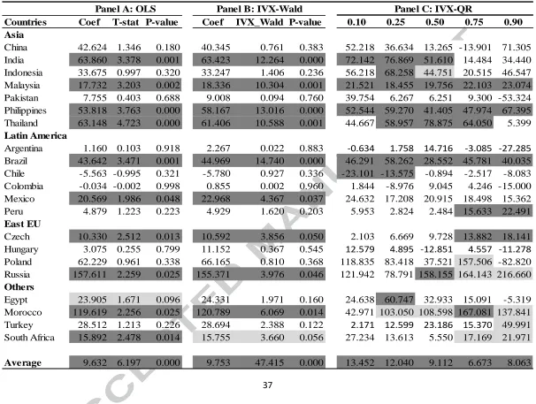
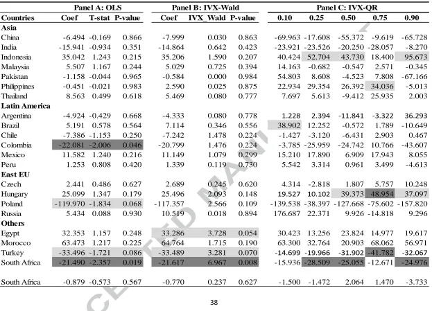
We repeat our previous regressions with net flows, and find that the results of
contemporaneous predictability are similar to those based on gross inflows (as shown from
Tables 4 -5). Nevertheless, we observe even less evidence of one-month-ahead
predictability—both in sample and out-of-sample, both through the conditional mean and
conditional quantile regressions. Therefore, such results may again justify our choice of gross
inflows.
[Insert Table 4 – 5 around here]
Equity flows in our main empirical analysis are measured in USD (deflated by CPI).
However, Curcuru et al. (2011) argue that such a specification may lead to confounding
results because of the wealth effect: if financial wealth is growing—which is a reasonable
assumption—a dollar today may suggest significantly different value in ten years. To
investigate this possibility, we scale equity flows with gross domestic productivity (GDP),
which is a standard method from the literature (e.g., Yan et al., 2016). Nevertheless, we
refrain from choosing this specification as the baseline specification in our main analysis
because GDP data are available at much lower frequency. The results are reported from
Tables 7 to 8. One can observe that the results are similar with those from our main analysis;
such findings may imply a relatively small impact of the wealth effect on our main analysis.
[Insert Table 6 – 7 around here]
4.2. Out-of-sample tests
Next, we investigate equity flows’ out-of-sample forecasting ability from the two countries
where equity flows could help to predict one-month-ahead returns (in-sample). Our
motivation is that, firstly, a large number of studies suggest that there is no necessary
association between in-sample and out-of-sample predictability (see, e.g., Welch and Goyal,
2007). Secondly, practitioners might be much more interested in out-of-sample forecasting.
19
to see whether predictive regression of equity flows could outperform a prevailing-mean
model. Specifically, corresponding to each country, we first compute the one-month-ahead
forecast using equity flows as a predictor. This takes the form as:
, (7)
where and are the OLS estimates of intercept and slope coefficient (for equity
flows), respectively. We use Newey-West robust standard errors to account for serial
correlation and heteroscedasticity. For each out-of-sample evaluation, the data is collected
from the start of the sample through month t. Next, we compare the one-month-ahead
forecasted return from the benchmark model (prevailing mean), which is calculated as
the average excess returns from the beginning of the sample through month t. Formally, it can
be written as below:
, (8)
In fact, the prevailing mean forecast is equivalent to the constant expected excess
return model in Equation (7) with . If the benchmark model outperforms our predictive
regression with equity flows, it would suggest that equity flows might not help to forecast
future returns, such that it might be even better to calibrate returns time series with a random
walk with drift. We compare the performance of these two models by comparing their Mean
Squared Forecast Error (MSFE), which is also called as the out-of-sample R-squared
statistics (Rapach et al., 2016). The period for out-of-sample evaluation is between January
2003 and December 2014. We use the statistics of Clark and West (2007) to test whether our
predictive regression forecast delivers a significant improvement in MSFE. The null
hypothesis of this test is that the benchmark (prevailing mean) MFSE is less than or equal to
the predictive regression MSFE. This is corresponding to , where
represents the out-of-sample R-squared statistics (Rapach et al., 2016). If we could reject
20
the predictive regression, then we can conclude that our predictive regression with equity
flows as the regressor can outperform the benchmark model, thus international equity flows
might contain relevant information to forecast future stock returns in EMEs.
[Insert Table 8 around here]
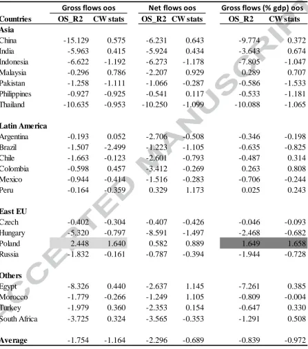
Table 8 shows our sample test results. In Column (1), we notice that the
out-of-sample R-squared are almost all negative in all countries except Poland, which implies that
equity flows to all these countries fail to outperform the prevailing mean benchmark model.
In other words, equity flows to these countries might not be helpful to forecast future stock
returns. Moreover, equity flows to South Africa lack significance in the out-of-sample test,
even though the in-sample results are significant. Therefore, this observation confirms the
conclusion of Welch and Goyal (2007) that in-sample predictability would not necessarily
lead to out-of-sample forecasting ability, in which practitioners might be more interested.
Finally, Poland seems to be the only remnant in our out-of-sample test. Yet, its significance is
only at 10% level, even though its test statistics of Clark and West (2007) is close to 5%
critical value. Overall, we find little evidence for the out-of-sample stock predictability of
foreign investors in EMEs.
4.3. Trading strategies based on portfolio sorting
By focusing on the contemporaneous regressions, it would be useful to see whether the
contemporaneous relation leads to a successful trading strategy. We sort the stock indices
into 5 quintiles according to their (12-month, 26-month, and 60-month) rolling OLS betas on
foreign equity flows and long each quintile with equal weights. Table 9 reports the results.
The second column shows the mean of rolling OLS betas, while the last column shows the
mean of number of EMEs in each quintile. Ret1, Ret12, Ret24, Ret36, Ret48 and Ret60
denote the cumulative buy-and-hold returns on a rolling window of 1, 12, 24, 36, 48 and 60
21
intertemporal results, we could not find a pattern for any of the cumulative buy-and-hold
returns at any horizons, no matter we use 12-month, 26-month, or 60-month rolling OLS
betas on capital flows. We have also tried to repeat this exercise with the top and bottom 25%
returns for each country, and the results are qualitatively similar. Overall, we find difficulty in
building a profitable trading strategy based on past rolling OLS betas on foreign equity flows.
4.4. Average global equity flows and stock market returns in EMEs
Is there a way to capture the effect of the U.S. as a global leader in driving stock market
returns in EMEs? In addition to individual equity flows, we look into the average global
equity flow that may capture the effect of the U.S. (proxying a global factor). The results
from this averaged scenario further confirms our results for each individual country in every
table. We thank a referee for pointing it out. For a study of the effect of the U.S. stock market
on international stock markets, see Rapach et al. (2013).
5. Concluding remarks
Global capital flows have significantly increased during the past two decades. Short-term
capital flows, especially international equity flows, have a substantial impact on the stock
markets in EMEs. Motivated by this conjecture, this paper seeks to investigate the
interrelationship between international equity flows and the stock returns in EMEs.
To conduct our empirical analysis, we collect monthly data for 21 EMEs over
1995-2014. We employ both in-sample and out-of-sample tests to investigate our research question.
As the exact degree of a predictor’s persistence is not usually precisely identifiable, standard
unit root test might not provide a firm guide (Lee, 2016). Therefore, we should employ
predictive regressions, which could handle various degrees of persistence. To that end, this
paper employs the state-of-art predictive regression models based on IVX-instrumentation, to
ensure that our empirical results would not be a statistical artifact due to a persistent regressor.
22
stock returns among a large number of EMEs. This observation is especially prominent in
Asian countries. Moreover, equity flows’ estimated coefficients are mostly positive. All of
these observations seem to confirm the immediate price impact of equity flows towards
EMEs.
However, there is neither in-sample nor out-of-sample evidence that international
equity flows could predict one-month-ahead stock returns. Among the a few countries where
equity flows display significant estimates, their coefficients are negative and counter-intuitive.
These observations imply that equity flows’ price impact is not persistent: when equity flows
rush into EMEs, they drive up prices contemporaneously but not persistently12.
Our finding have important implications. Regarding flows equity flows, policymakers’
attention should be more on their concurrent consequences than their future profitability. The
remarkable turmoil in emerging stock markets during the GFC is a reminder of the
importance of investigating their dynamics (e.g., Fuertes et al., 2016; Yan et al., 2016; Fuertes
et al., 2017). We find difficulty in building a profitable trading strategy based on past rolling
OLS betas on foreign equity flows.
There are some caveats to our investigation. Ideally, we should have considered other
variables that may influence stock market returns. Additional variables include dividend yield
and earning-price ratio (e.g., Rapach et al., 2016). However, the poor availability and quality
of these fundamental variables for EMEs hinder our further investigation. We choose to avoid
fundamentals in this study due to the poor quality of data in EMEs. We suspect that there
might be a problem of misreporting, for we could observe a considerable amount of zero
dividends for some countries. For example, Pakistan’s dividends data start with January 1995,
but it shows a series of zeros between November 1996 and May 1998—it might be unlikely
for a whole nation to experience zero dividends for such a long time. For this reason, we use
12
23
data of prices only. We choose to focus on the EMEs in this paper, as they are still segregated
from the developed markets, albeit the dramatic globalization over the past decades (e.g.,
Bekaert and Harvey, 2017). Our method can be used for other markets. Due to data limitation,
we cannot rule out the possibility of predictability at a higher frequency in equity flows as
well as other types of flows. Flows at higher frequency are more persistent, and there is a
greater need for the tools we have introduced to this topic in this paper. We leave this work
24
6. Appendix.
This section discusses the potential problems associated with the traditional OLS approach.
We first document the problem and present the solutions after that.
6.1. Statistical Inference in the Presence of Persistent Regressors
We start our analysis with ordinary least squares (OLS) regression, which is standard in the literature of predicting stock returns. The regression model is shown as:
.
(A.1)
In this regression, usually represents contemporaneous stock returns, and denotes the lag of a vector of financial variables, which contains equity flows only in our case. A number of early findings based on such regressions report that the t-statistic is typically large enough to reject the null hypothesis that . Thus, they suggest a strong evidence of stock return predictability. However, Campbell and Yogo (2006) doubt the validity of such tests and further show that they tend to reject the null too frequently when the predictor variable is persistent and the innovations are highly correlated with returns.
Regarding the degrees of persistence of the predictor, we follow the presentations from Kostakis et al. (2015) and Lee (2016). We firstly assume that the vector of predictors
has the following autoregressive form:
(A.2)
,
(A.3)
where n is the sample size and if we have K predictors. According to Equation (A.3), the pair determines predictors’ persistence. In particular, Lee (2016) shows that can belong to any of the following persistence categories:
(I0) Stationary: and ,
25
(I1) Local to unity and unit root: and , ,
(ME) Mildly explosive: and , .
If any predictor falls into the category of (I1) or even (ME), its persistence will lead to size distortion of the empirical results, as reported in the literature. On the other hand, Section 1 (Introduction) of this paper has briefly introduced the persistent nature of equity flows and the difficulty to identify the exact degree of their persistence empirically. Next, we show our solution by employing recent predictive regression based on IVX-filtering instrumentation.
6.2. Solutions: IVX filtering
The literature has developed two major approaches to correct the nonstandard distortion caused by persistent predictors. The first approach focuses on the Bonferroni method (e.g., Cavanagh et al., 1995; Campbell and Yogo, 2006). Its main idea is to find a confidence interval (CI) for that incorporates confidence limits for c (shown in Equation A.3). In this way, the model can be independent of any particular value of c (Phillips, 2015). However, this method has several disadvantages: firstly, such models usually allow for only one predictor in the regression. More importantly, Phillips (2015) and Lee (2016) show that these models may lose validity when predictor persistence falls between (MI) and (I0). For this reason, it would be particularly difficult to employ models based on the Bonferroni method in our study, since it is empirically difficult to identify the exact degree of capital flows’ persistence. Therefore, models retaining their validity over various degrees would be more desirable.
A solution to this problem is provided by the IVX filtering method of Phillips and Magdalinos (2009), which has been employed by recent studies such as Kostakis et al. (2015) and Lee (2016). These models can handle predictor variables with various degrees of persistence. The basic idea is to filter a predictor with strong persistence (e.g., belonging to the parameter space of I (1) into an instrument with mildly integrated (MI) persistence. Specifically, following the presentation from Lee (2016), we filter persistent data to generate :
26
When , . In this case, the instrument is equivalent to the first difference of the persistent predictor, which is one of the most common ways to remove persistence. Although first difference could wipe out the nonstandard distortion, its sacrifice is a substantial loss of power. On the other hand, when then , we simply use level data without any filtering. In this case, the power is retained, but the resulting persistence would lead to a distorted inference as we discussed earlier.
To exploit advantages both from using level and the first difference of persistent predictor, the IVX-method filters to generate with (MI) persistence, intermediate between I(0) and I(1). Specifically, we choose so that:
(A.5)
,
(A.6)
where , , and .
27
References
Albuquerque, R., Bauer G. H., & Schneider. M. (2007) International equity flows and returns: A quantitative equilibrium approach. Review of Economic Studies 74(1): 1-30.
Albuquerque, R., Bauer, G. H., & Schneider, M. (2009). Global private information in international equity markets. Journal of Financial Economics, 94(1): 18–46.
Ahmed, S., & Zlate, A. (2014). Capital flows to emerging market economies: A brave new world? Journal of International Money and Finance, 48, 221-248.
Bekaert, G., & Harvey, C. R. (2017). Emerging equity markets in a globalizing world. SSRN working paper. Available at SSRN: https://ssrn.com/abstract=2344817.
Bekaert, G., Harvey, C. R., & Lumsdaine, R. L. (2002). The dynamics of emerging market equity flows, Journal of International Money and Finance 27, 295-350.
Bohn, H., & Tesar, L. L. (1996). US equity investment in foreign markets: Portfolio rebalancing or return-chasing? American Economic Review, 86(2), 77-81.
Broner, F. A., Gelos, R. G., & Reinhart, C. M. (2006). When in peril, retrench: Testing the portfolio channel of contagion. Journal of International Economics, 69(1), 203-230. Brennan, M. J., & Cao, H. H. (1997). International portfolio investment flows. Journal of
Finance, 52(5), 1851-1880.
Campbell, J. Y., & Yogo, M. (2006). Efficient tests of stock return predictability. Journal of Financial Economics, 81(1), 27-60.
Cavanagh, C. L., Elliott, G., & Stock, J. H. (1995). Inference in models with nearly integrated regressors. Econometric Theory, 11(5), 1131-1147.
Cenedese, G., Sarno, L., & Tsiakas, I. (2014). Foreign exchange risk and the predictability of carry trade returns. Journal of Banking & Finance, 42 (C), 302-313.
Cenedese, G., & Mallucci, E. (2016). What moves international stock and bond markets? Journal of International Money and Finance, 60, 94-113.
Clark, T. E., & West, K. D. (2007). Approximately normal tests for equal predictive accuracy in nested models. Journal of Econometrics, 138(1), 291-311.
Curcuru, S. E., Thomas, C. P., Warnock, F. E., & Wongswan, J. (2011). US international equity investment and past and prospective returns. American Economic Review, 101(7), 3440-3455.
28
Dumas, B., Lewis, K. K., & Osambela, E. (2017). Differences of opinion and international equity markets. Review of Financial Studies, 30(3), 750-800.
Forbes, K. J. (2013). The “Big C”: Identifying and mitigating contagion. Jackson Hole
Symposium Hosted by the Federal Reserve Bank of Kansas City.
Forbes, K. J., & Warnock, F. E. (2012). Capital flow waves: Surges, stops, flight, and retrenchment. Journal of International Economics, 88(2), 235-251.
Froot, K.A., O’Connell, P., & Seasholes M.S. (2001). The portfolio flows of international investors. Journal of Financial Economics 59, 151–194.
Fuertes, A. M., Phylaktis, K., & Yan, C. (2016). Hot money in bank credit flows to emerging markets during the banking globalization era. Journal of International Money and Finance, 60, 29-52.
Fuertes, A. M., Phylaktis, K., & Yan, C. (2017). Uncovered equity “disparity” in emerging markets, Cass Business School working paper.
Ghosh, A. R., Qureshi, M. S., Kim, J. I., & Zalduendo, J. (2014). Surges. Journal of International Economics, 92(2), 266-285.
Griffin, J. M., Nardari, F., & Stulz, R. M. (2004). Are daily cross-border equity flows pushed or pulled? Review of Economics and Statistics, 86(3), 641-657.
Hau, H., & Rey, H. (2004). Can portfolio rebalancing explain the dynamics of equity returns, equity flows, and exchange rates? American Economic Review, 94(2), 126-133.
Hau, H. & Rey, H. (2006). Exchange rates, equity prices and capital flows. Review of Financial Studies 19, 273–317.
Jotikasthira, C., Lundblad, C., & Ramadorai, T. (2012). Asset fire sales and purchases and the international transmission of funding shocks. Journal of Finance, 67(6), 2015-2050. Kamin, S. B., and DeMarco L. P. (2012). How did a domestic housing slump turn into a
global financial crisis? Journal of International Money and Finance 31, 10-41. Koenker, R., & Bassett Jr, G. (1978). Regression quantiles. Econometrica, 46(1), 33-50. Kostakis, A., Magdalinos, T., & Stamatogiannis, M. P. (2015). Robust econometric inference
for stock return predictability. Review of Financial Studies, 28(5), 1506-1553.
Kyle, A. S. (1985). Continuous auctions and insider trading. Econometrica, 53(6), 1315-1335. Lee, J. H. (2016). Predictive quantile regression with persistent covariates: IVX-QR
approach. Journal of Econometrics, 192(1), 105-118.
Phillips, P. C., & Magdalinos, T. (2009). Econometric inference in the vicinity of unity.
29
Phillips, P. C. (2015). Halbert White Jr. Memorial JFEC Lecture: Pitfalls and Possibilities in Predictive Regression. Journal of Financial Econometrics, 13(3), 521-555.
Phillips, P. C., & Lee, J. H. (2016). Robust econometric inference with mixed integrated and mildly explosive regressors. Journal of Econometrics, 192(2), 433-450.
Puy, D. (2016). Mutual funds flows and the geography of contagion. Journal of International Money and Finance, 60, 73-93.
Raddatz, C., & Schmukler, S. L. (2012). On the international transmission of shocks: Micro-evidence from mutual fund portfolios. Journal of International Economics, 88(2), 357-374.
Rapach, D. E., Strauss, J. K., & Zhou, G. (2013). International stock return predictability: What is the role of the United States? Journal of Finance, 68(4), 1633-1662.
Rapach, D. E., Ringgenberg, M. C., & Zhou, G. (2016). Short interest and aggregate stock returns. Journal of Financial Economics, 121(1), 46-65.
Richards, A. (2005). Big fish in small ponds: The trading behavior and price impact of foreign investors in Asian emerging stock markets. Journal of Financial and Quantitative Analysis, 40(01), 1-27.
Rothenberg, A. D., & Warnock, F. E. (2011). Sudden flight and true sudden stops. Review of International Economics, 19(3), 509-524.
Sarno, L., & Taylor, M. P. (1999a). Hot money, accounting labels and the permanence of capital flows to developing countries: an empirical investigation. Journal of Development Economics, 59(2), 337-364.
Sarno, L., & Taylor, M. P. (1999b). Moral hazard, asset price bubbles, capital flows, and the East Asian crisis: The first tests, Journal of International Money and Finance 18, 637-657.
Sarno, L., Tsiakas, I., & Ulloa, B. (2016). What drives international portfolio flows? Journal of International Money and Finance, 60, 53-72.
Tillmann, P. (2013). Capital inflows and asset prices: Evidence from emerging Asia. Journal of Banking & Finance, 37(3), 717-729.
Tong, H., & S. Wei (2011). The composition matters: Capital inflows and liquidity crunch during a global economic crisis. Review of Financial Studies 24(6), 2023-2052.
Ulku, N. & Weber, E. (2014). Identifying the interaction between foreign investor flows and emerging stock market returns, Review of Finance, 18(4): 1541-158.
30
Welch, I., & Goyal, A. (2007). A comprehensive look at the empirical performance of equity premium prediction. Review of Financial Studies, 21(4), 1455-1508.
[image:32.595.72.529.80.478.2]
31
32
Table 1. Summary Statistics. This table reports the summary statistics of the key variables in this study. Mean and S.D. denote the mean value and standard deviation, respectively. Stock returns are computed from MSCI Index. Equity flows are in millions of USD.
Countries Mean S.D. Mean S.D. Mean S.D.
Asia
China (PRC) 0.109 9.896 30.137 337.104 0.002 0.014 India 0.525 8.822 76.576 257.698 0.010 0.031 Indonesia 0.745 13.179 23.581 84.790 0.006 0.031 Malaysia 0.114 8.626 30.380 108.445 0.022 0.096 Pakistan 0.244 10.979 3.104 19.312 0.004 0.024 Philippines 0.006 8.629 9.100 31.519 0.010 0.034 Thailand 0.119 11.014 20.780 77.927 0.010 0.037
Argentina 0.604 11.498 1.857 137.226 0.001 0.048 Brazil 0.606 10.660 291.838 655.139 0.029 0.058 Chile 0.049 6.699 8.178 81.623 0.006 0.073 Colombia 0.642 9.086 5.300 60.974 0.003 0.034 Mexico 0.049 6.699 -35.686 253.960 -0.005 0.040 Peru 0.858 8.635 10.537 93.137 0.014 0.144
East EU
Czech 0.498 8.279 -5.814 62.823 -0.007 0.099 Hungary 0.783 10.634 0.219 26.464 0.001 0.039 Poland 0.489 10.231 7.937 20.981 0.003 0.009 Russia 1.456 15.142 -1.178 73.542 0.000 0.012
Others
Egypt 0.914 9.449 2.308 29.736 0.004 0.035 Morocco 0.157 5.484 0.350 3.372 0.001 0.007 Turkey 1.385 14.822 22.572 127.594 0.009 0.052 South Africa 0.288 7.680 29.356 104.053 0.017 0.060
Average 0.507 6.388 531.431 987.040 0.145 0.269
Gross flows
Excess return Gross flows (% gdp)
[image:33.595.75.527.117.631.2][image:34.842.135.708.105.562.2]
33
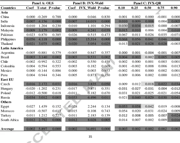
Table 2. Gross flows and contemporaneous stock returns. Stock returns are computed from MSCI Index. Equity flows are in millions of USD. Panel C reports the results of estimated coefficients. Light and dark gray denote 10% and 5% significance level, respectively.
Countries Coef T-stat P-value Coef IVX_Wald P-value 0.10 0.25 0.50 0.75 0.90
Asia
China 0.000 -0.172 0.864 0.000 0.024 0.876 0.001 -0.001 -0.001 -0.001 0.004
India 0.007 3.400 0.001 0.007 11.393 0.001 0.010 0.009 0.007 0.002 0.005
Indonesia 0.011 1.307 0.193 0.012 1.336 0.248 0.029 0.034 0.015 0.000 0.010
Malaysia 0.015 4.035 0.000 0.015 9.124 0.003 0.018 0.015 0.010 0.015 0.016
Pakistan 0.021 0.793 0.428 0.023 0.372 0.542 0.067 0.011 0.027 0.043 -0.068
Philippines 0.058 3.706 0.000 0.061 12.140 0.000 0.062 0.062 0.048 0.043 0.063
Thailand 0.025 3.642 0.000 0.024 6.922 0.009 0.018 0.026 0.030 0.024 0.004
Latin America
Argentina 0.000 -0.113 0.910 0.000 0.000 0.995 0.000 0.001 -0.001 -0.001 -0.010
Brazil 0.003 3.032 0.003 0.003 9.141 0.002 0.004 0.003 0.002 0.005 0.005
Chile -0.008 -1.498 0.135 -0.008 2.293 0.130 -0.019 -0.015 -0.004 -0.002 -0.005
Colombia -0.003 -0.327 0.744 -0.003 0.068 0.795 0.001 -0.009 0.008 0.003 -0.013
Mexico 0.003 1.587 0.114 0.003 2.667 0.102 0.004 0.002 0.001 0.003 0.001
Peru 0.007 1.205 0.229 0.007 1.232 0.267 0.012 0.006 0.003 0.018 0.024
East EU
Czech 0.021 3.124 0.002 0.021 6.087 0.014 0.015 0.013 0.018 0.026 0.034
Hungary 0.007 0.374 0.709 0.014 0.298 0.585 0.021 0.010 -0.028 0.005 -0.012
Poland 0.005 0.176 0.860 0.008 0.057 0.811 0.037 0.029 0.008 0.061 -0.031
Russia 0.034 3.022 0.003 0.034 6.697 0.010 0.023 0.034 0.028 0.031 0.040
Others
Egypt 0.032 1.794 0.074 0.033 2.549 0.110 0.054 0.055 0.042 0.018 -0.008
Morocco 0.200 1.626 0.105 0.204 3.783 0.052 0.069 0.137 0.213 0.305 0.239
Turkey 0.011 1.182 0.239 0.011 2.041 0.153 0.001 0.009 0.006 0.007 0.023
South Africa 0.010 2.397 0.017 0.010 3.965 0.046 0.014 0.007 0.003 0.008 0.014
Average 0.002 5.550 0.000 0.003 41.086 0.000 0.003 0.003 0.003 0.002 0.002
Panel C: IVX-QR
[image:35.842.135.711.106.561.2]
34
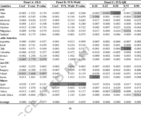
Table 3. Gross flows and one-month-ahead stock returns. Stock returns are computed from MSCI Index. Equity flows are in millions of USD. Panel C reports the results of estimated coefficients. Light and dark gray denote 10% and 5% significance level, respectively.
Countries Coef T-stat P-value Coef IVX_Wald P-value 0.10 0.25 0.50 0.75 0.90
Asia
China -0.002 -1.151 0.251 -0.002 0.998 0.318 -0.002 -0.004 -0.003 -0.001 -0.001
India -0.001 -0.564 0.573 -0.001 0.209 0.648 0.006 0.003 -0.002 -0.005 -0.005
Indonesia 0.004 0.597 0.551 0.004 0.194 0.660 0.020 0.004 0.006 0.003 -0.026
Malaysia 0.005 1.270 0.205 0.005 0.856 0.355 0.011 0.006 0.005 0.002 0.000
Pakistan -0.001 -0.033 0.974 0.000 0.000 0.999 0.052 0.008 -0.007 0.019 -0.080
Philippines 0.000 0.023 0.982 0.003 0.023 0.878 0.020 0.009 0.022 0.029 -0.005
Thailand 0.002 0.210 0.834 0.001 0.005 0.945 0.002 0.000 -0.006 0.011 -0.009
Latin America
Argentina -0.003 -0.742 0.459 -0.002 0.207 0.649 0.000 0.001 -0.004 -0.007 0.010
Brazil 0.000 0.324 0.746 0.000 0.145 0.703 0.003 0.001 0.000 0.000 -0.001
Chile -0.006 -0.915 0.361 -0.006 1.185 0.276 -0.020 -0.004 -0.007 0.004 0.001
Colombia -0.012 -1.960 0.051 -0.012 1.439 0.230 -0.003 -0.018 -0.011 0.011 -0.026
Mexico 0.002 1.231 0.220 0.002 1.032 0.310 0.002 0.003 0.001 0.003 0.001
Peru 0.001 0.505 0.614 0.002 0.069 0.793 0.008 0.006 0.002 -0.004 -0.009
East EU
Czech 0.002 0.274 0.784 0.002 0.081 0.776 0.008 -0.005 0.003 -0.003 -0.012
Hungary 0.018 0.640 0.523 0.018 0.478 0.489 -0.024 0.011 0.030 0.042 0.051
Poland -0.068 -2.173 0.031 -0.067 4.528 0.033 -0.049 -0.042 -0.059 -0.055 -0.054
Russia 0.010 0.957 0.339 0.011 0.678 0.410 0.043 0.020 0.002 0.005 0.008
Others
Egypt 0.029 1.020 0.309 0.030 2.189 0.139 0.037 0.018 0.032 -0.005 -0.002
Morocco 0.124 1.076 0.283 0.128 1.477 0.224 0.086 0.099 0.034 0.160 0.101
Turkey -0.012 -1.626 0.105 -0.012 2.505 0.113 -0.002 -0.007 -0.016 -0.010 -0.014
South Africa -0.011 -2.012 0.045 -0.011 4.892 0.027 -0.008 -0.015 -0.019 -0.006 -0.013
Average 0.000 -0.616 0.538 0.000 0.240 0.624 -0.002 -0.001 0.001 0.000 -0.001
Panel C: IVX-QR