Harmonic phase path integral approximation of thermal quantum correlation functions

warwick.ac.uk/lib-publications

Original citation:

Robertson, Christopher and Habershon, Scott. (2018) Harmonic-phase path-integral

approximation of thermal quantum correlation functions. The Journal of Chemical Physics,

148 (10). 102316.

Permanent WRAP URL:

http://wrap.warwick.ac.uk/94752

Copyright and reuse:

The Warwick Research Archive Portal (WRAP) makes this work by researchers of the

University of Warwick available open access under the following conditions. Copyright ©

and all moral rights to the version of the paper presented here belong to the individual

author(s) and/or other copyright owners. To the extent reasonable and practicable the

material made available in WRAP has been checked for eligibility before being made

available.

Copies of full items can be used for personal research or study, educational, or not-for-profit

purposes without prior permission or charge. Provided that the authors, title and full

bibliographic details are credited, a hyperlink and/or URL is given for the original metadata

page and the content is not changed in any way.

Publisher’s statement:

This article may be downloaded for personal use only. Any other use requires prior

permission of the author and AIP Publishing.

The following article appeared in Robertson, Christopher and Habershon, Scott. (2018)

Harmonic-phase path-integral approximation of thermal quantum correlation functions. The

Journal of Chemical Physics, 148 (10). 102316 and may be found at

https://doi.org/10.1063/1.5002189

A note on versions:

The version presented in WRAP is the published version or, version of record, and may be

cited as it appears here.

Harmonic-phase path-integral approximation of thermal quantum

correlation functions

Christopher Robertsona)_{and Scott Habershon}a)

Department of Chemistry and Centre for Scientific Computing, University Of Warwick, Coventry CV4 7AL, United Kingdom

(Received 30 August 2017; accepted 9 October 2017; published online 10 November 2017)

We present an approximation to the thermal symmetric form of the quantum time-correlation function in the standard position path-integral representation. By transforming to a sum-and-difference position representation and then Taylor-expanding the potential energy surface of the system to second order, the resulting expression provides a harmonic weighting function that approximately recovers the contribution of the phase to the time-correlation function. This method is readily implemented in a Monte Carlo sampling scheme and provides exact results for harmonic potentials (for both linear and non-linear operators) and near-quantitative results for anharmonic systems for low temperatures and times that are likely to be relevant to condensed phase experiments. This article focuses on one-dimensional examples to provide insights into convergence and sampling properties, and we also discuss how this approximation method may be extended to many-dimensional systems.Published by AIP Publishing.https://doi.org/10.1063/1.5002189

I. INTRODUCTION

Algorithms that employ the path-integral formulation of quantum statistical mechanics1–4_{have become invaluable tools} for calculating time-independent thermal expectation values of quantum-mechanical operators, bridging the gap between the exponential-scaling wavefunction propagation methods and purely classical approaches for estimating thermody-namic observables. To date, path-integral molecular dythermody-namics (PIMD) and path-integral Monte Carlo (PIMC) have been used to study quantum contributions to time-independent thermal equilibrium properties for a wide range of condensed-phase systems.4–21However, whileexact time-independent proper-ties can be calculated readily by PIMC or PIMD, path-integral evaluation of time-correlation functions (TCFs), allowing cal-culation oftime-dependentproperties, such as diffusion coef-ficients, scattering cross sections, dipole relaxation times, and reaction rates, remains an enormous challenge, principally as a result of the appearance of the so-called “sign problem” arising due to the action of quantum time propagators.20,22–49

Rather than seeking to address the sign problem directly, several successful simulation methods have shown that, for many systems, quantum dynamical properties can be well-approximated by assuming that explicit quantum coherent effects are “washed out” by the thermal environment, with the main quantum effect arising due to statistical fluctuations associated with zero-point energy (ZPE) conservation and tun-neling. In this vein, methods such as ring-polymer molecular dynamics (RPMD8,11,27,33,50–70), centroid molecular dynam-ics (CMD20,35,37,38,71–73), and the linearised semi-classical initial value representation (LSC-IVR42,43,45,48,49,74–77_{) have}

a)_{Electronic addresses: [email protected] and S.Habershon@}

warwick.ac.uk

proven to be enormously successful in modeling dynamic properties (via approximation of time-correlation functions) in a variety of condensed-phase systems represented by both model Hamiltonians and more accurate ab initio methods.

While methods such as RPMD, CMD, and LSC-IVR are appealing, principally due to both their physically consis-tent predictions and computational tractability, these approx-imations are not universally applicable. For example, it is well-known that RPMD time-correlation functions can exhibit spurious non-physical vibrational spectra,27,38,57_{and the} asso-ciated treatment of non-linear operators is similarly challeng-ing;65 _{it is worth noting that these problems have been} dra-matically reduced by the recent introduction of thermostated RPMD (TRPMD78), although the introduction of an artificial broadening into associated vibrational spectra demonstrates that this approach is not a “cure-all.” Similarly, vibrational spectra calculated by CMD can exhibit the so-called “cur-vature problem,”38 while methods based on propagation of classical trajectories, such as LSC-IVR, can demonstrate the “ZPE-leakage problem.”57Finally, in all cases (RPMD, CMD, and LSC-IVR), the neglect of explicit quantum coherence sug-gests that treatment of systems where this feature is prominent (e.g., coupled nuclear-electronic dynamics) remains challeng-ing (although it is worth highlightchalleng-ing that progress is bechalleng-ing made in this direction too33,53,79_).

In this article, we present a further path-integral-based approximation of thermal quantum time-correlation functions that shows some promise for treating systems where explicit quantum phase interference might be important. Taking inspi-ration from much of the previous work on using Monte Carlo approaches to sample real-time quantum dynamics, we start from the symmetrized complex form of the quantum time-correlation function in the standard position path-integral

representation. In calculating the TCF, we transform the sys-tem coordinates to a sum-and- difference representation and subsequently Taylor-expand the potential energy of the sys-tem to second order around the “sum” path; in other words, we make a harmonic assumption for the potential energy sur-face in the “difference” coordinates. This approach enables one to explicitly evaluate the TCF integral over the “dif-ference” coordinates. The resulting expression for the TCF provides one with a weighting function that approximately recovers the contribution of the phase to the TCF integral and which lies near the configurational space associated with the minimisation of the action. We show that under the har-monic assumption noted above, this approximation can ade-quately calculate TCF for anharmonic potentials. We refer to this approach as harmonic-phase approximation Monte Carlo (HPA-MC).

We note that our approach is similar to some already exist-ing in the literature22_{but has some advantages; for example,} HPA-MC does not require averaging over complex phases, as in recent approaches such as the partially linearised den-sity matrix method.80_{Furthermore, HPA-MC does not require} propagation of classical trajectories (and the inevitable ZPE leakage problem); in fact, as noted above, exact treatment of the Boltzmann operator is built into our approach (although the harmonic approximation in calculation of the TCF inevitably introduces errors, as discussed later). We note that HPA-MC gives the exact result for any harmonic system, for any oper-ator; the non-linear operator problems which can appear in RPMD and CMD do not operate in HPA-MC. Importantly, we also find that HPA-MC can provide near-quantitative results for anharmonic PESs (Sec. II C) for low temperatures. It, nevertheless, suffers from accumulation of errors which only allows one to adequately approximate TCF for moderate real-times. The times and temperatures treated here are nevertheless relevant to condensed phase systems, and HPA-MC might prove to be an efficient approach for calculating transport properties for these. We conclude this article with a discus-sion of how HPA-MC might be improved upon and extended to higher-dimensional systems, work which is currently ongoing.

II. THEORY

We begin by briefly outlining the main concepts relat-ing to quantum time-correlation functions which are relevant to this work. Then, we discuss the origin of the HPA-MC approach, before highlighting how this approach can enable efficient approximation of TCFs.

A. Quantum time-correlation functions

The standard quantum time-correlation function for two operators ˆAand ˆBis given by

CAB(t)=

1 ZTr

e−βHˆAeˆ +iHtˆ/~_Beˆ −iHtˆ /~

, (1)

where β =1/(kbT),Z is the partition function, and ˆH is the

Hamiltonian for the system, assumed throughout to be of the standard form ˆH=Tˆ+ ˆV, where ˆTis the nuclear kinetic energy operator and ˆV is the potential energy operator. Straightfor-ward application of the path-integral approach to evaluate both imaginary-time and real-time propagator matrix ele-ments results in an expression which requires averaging over a complex phase-factor, leading to the usual “sign problem.”

An alternative TCF which is more amenable to MC inte-gration is obtained by replacing t → t+iβ~/2, giving the

thermal symmetric TCF of the form,81

GAB(t)=CAB(t+iβ~/2)

= 1

ZTr

ˆ

Ae+iHˆτ∗/~_Beˆ −iHˆτ/~

, (2)

whereτ=t−iβ_~/2. The two correlation functionsG_AB(t) and CAB(t) are related through their Fourier transforms such that

GAB(ω)=e−β~/2CAB(ω).

In GAB(t), the propagator elements hx|e−iHˆτ ∗_/

~_|x0_{i and}

hx0_|e−iHˆτ/~_{|xi are complex conjugates, resulting in a real,}

positive-definite sampling function which enables MC integra-tion. A number of approaches have shown this to be a fruitful avenue towards semiclassical approaches.22,82Specifically, the path-integral form ofGAB(t) is83

GAB,P(t)=

1 Z

dx1. . .dx2PA(x1)B(xP+1)ρ(x1,. . .,x2P)eiΦ(x1,...,x2P),

ρ(x1,. . .,x2P)=(

mP 2π|τ|_~)

P

exp

     

− mPβ 4|τ|2

~2 2P

X

k=1

(xk+1−xk)2− β 2P

2P

X

k=1

V(xk)      

,

Φ(x1,. . .,x2P)=

mPt 2~|τ|2

     

P

X

k=1

(xk+1−xk)2− 2P

X

k=P+1

(xk+1−xk)2      

− t

~P      

P

X

k=2

V(xk)− 2P

X

k=P+2

V(xk)      

.

(3)

In Eq. (3) (and hereafter), we restrict our attention to one-dimensional systems for notational convenience; furthermore, we have assumed that each propagator matrix element in Eq. (2) has been discretised into P “slices,” leading to 2P “slices” (or beads) to be sampled in total. The function ρ(x) defines a sampling function for the coordinates of a ring-polymer under the influence of the PES and can be used to

perform MC/MD estimation ofGAB23via

GAB(t)=

hA(x1)B(xP+1)eiΦiρ

heiΦ_iρ , (4)

gives rise to known difficulties, and a number of strategies have been devised to attempt to improve the convergence.30,82,84,85 Averaging over eiΦ _{gives rise to both positive and negative} contributions (i.e., appearance of the “sign problem”), and the denominator can approach zero for long times, making the integrals difficult to converge using standard simulation methods.

B. Harmonic-phase approximation

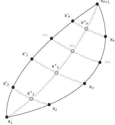
To escape the difficulties noted above, our approach is, to substituteeiΦ_{by a function, based on a harmonic} approx-imation, which approximately provides the correct weighting to a particular path, avoiding the highly oscillatory behaviour. To proceed, we turn to a “sum and difference” representation using the coordinates of adjacent “beads” along the forward and backward paths which emerge upon path-integral treat-ment of the propagator matrix eletreat-ments (Fig. 1). Here, let x_i0 = x2P+2−i, 2≤i≤P. A general orthogonal transformation

ofx_i0andxithat maintains a phase-space area must satisfy the

following constraint in the Jacobian,

dx dx+ _dxdx− dx0 dx+ dx

0 dx− =

a −b

a b

=1. (5)

Such transformations are given by

x =ax++ (1/2a)x−, x+= 1 2a(x+x

0

),

x0_=ax+_−(1/2a)x−_{, x}−_=a(x−x0_),

(6)

FIG. 1. Diagram showing the ring representing the forward and backward paths:{x,x0_{}beads are indexed in accord to their position away from bead} x1and rotated to obtainx+, the sum coordinates (the mean, ifa= 1).xnot displayed.

where a andb are fixed constants, and we refer to the x+ as “sum” coordinates andxas “difference” coordinates. For notational convenience, we definex₁+=x1andx+_P+1=xP+1.

Transforming to these new coordinates, the density and phase of Eq.(3)(omitting irrelevant pre-exponential factors) are now

ρ(x+

1,. . .,xP+1+ ,x − 2,. . .,x

− P)= exp

     

− mPβ 4|τ|2

~2     

2((x₁+−ax₂+)2+ (x_P+1+ −ax+_P)2+a2

P−1

X

k=2

(x+_k−x+_k+1)2)

+ 1 2a2((x

− 2)

2

+ (x_P−)2+

P−1

X

k=2

(x_k−−x_k+1− )2)    − β 2P (

V(x+₁) +V(x_P+1+ )

+

P−1

X

k=2

V(ax_k++ (1/2a)x−_k) +V(ax+_k−(1/2a)x−_k)          ,

Φ(x+₁,. . .,x_P+1+ ,x₂−,. . .,x−_P)= mPt

~|τ|2      

x₂+x₂−+x_P+x−_P−1 a(x

− 2x

+ 1+x

− Px

+ P+1) +

P−1

X

k=2

(x_k+1+ −x+_k)(x−_k+1−x_k−)

− t

~P( P

X

k=2

V(ax_k++ (1/2a)x_k−)−V(ax_k+−(1/2a)x−_k))

      . (7)

Equation(7)shows that the sum coordinatesx+ describe the average discretised path as a string coupled to the difference string defined byx.

To proceed, we now Taylor-expand the PES appear-ing in both the phase and the density about ax+, such that

V(x)≈V(ax+) + x

−

2a ! _∂V

∂x

x=ax+

+1 2

x−

2a

!2_∂2_V

∂x2 x=ax+

.

(8)

Noting that the PES at identically labelled beads,kappears in Eq.(7)as either a sum (in the case of density) or a difference (in the case of the phase), we find that

V(x) +V(x0_{)≈ 2V(ax}+_{) +}(x −

)2 4a2

∂2_V ∂x2 x=ax+

,

V(x)−V(x0_)≈ x −

a !∂_V

∂x

x=ax+

.

(9)

all odd orders ofx cancel out in the density ρ. Notice that for any choice of a, all derivatives ∂_∂n_xVn|x=ax+ are evaluated at the mean of the two beads, since ax+ = a(_2a1(x + x0))

=(1₂(x+x0)). We shall nevertheless find it convenient to use a=1/

√

2 when analysing the harmonic oscillator case (see the Appendix). We note that the transformation and second-order expansion performed so far remain exact for any harmonic PES. It can also be shown that for a cubic PES, a term is lost in the phase component, and for a quartic PES, terms in the phase and density parts are lost. For convenience, we now denote ∂_∂n_xVn|x=ax+= ∂

n_V+ ∂xn .

The upshot of this coordinate transformation and expan-sion is that the thermal symmetric TCF can be written as

GAB(t)=

1 Z

dx+dx−ρ+(x+)ρ−(x−)A(x1)B(xP+1)eiΦ 0_(x+_,x−₎

.

(10)

The “sum bead” contribution to the density is given by

ln(ρ+)=−mβPa

2

|τ|2 ~2

(

1 2a2((x

+ 1)

2_{+ (x}+ p+1)

2_{) + (x}+ p)2

− 1 a(x

+ p+1x

+ p+x+1x

+ 2) +

P−1

X

k=2

(x+_k)2−x_k+x_k+1+

+ |τ|

2 ~2

2ma2_P2 (V(x +

1) +V(x+P+1) + 2 P

X

k=2

V(ax_k+))   

.

(11)

Thus, ρ+(x+) provides a configurational sampling function which can be sampled by MC in a similar manner to the standard PIMC methodology, with the exception that ρ(x+) describes a “string polymer” rather than a “ring polymer.” Fur-thermore, the spring constants of Eq.(11)depend on both the inverse temperature βand the real timet, again in contrast to the standard PIMC/PIMD approach.

At this point, we do not appear to have made much progress in achieving a computationally tractable scheme when compared to Eq. (4). We would still have to sample configurations fromρ+_{ρand the ‘sign problem’e}iΦ0

remains. However, we now show that the coordinate transformation and harmonic expansion noted above enable one to analytically integrate out the dependence on thex coordinates, thereby removing the oscillatory nature of the integrand.

First, we note that that “difference bead” contribution to the density is given by

ln(ρ−(x−))= −mβP 4~2|τ|2a2

    

(x−_p)2+

P−1

X

k=2

(x−_k)2−x−_kx−_k+1

+|τ|

2 ~2

2mP2 P

X

k=2

(x−_k)2∂

2_V+

∂x2 k      . (12)

Twice differentiating this term gives an effective “Hessian” matrix for the difference string (omitting common factors) of the form

H0−=H−+ |τ|

2 ~2

mP2 1

~

∂2_V+ ∂x2

= * . . . . . ,

2 −1 0 · · · −1 2 −1

0 −1 2 .. . . .. + / / / / /

-+ |τ|

2 ~2

mP2 1

~

∂2_V+

∂x2 . (13)

The first matrix in Eq. (13),H, has analytical eigenvectors and eigenvalues of the form

U− ij =

r

2 Psin

π(i−1)(j−1) P

!

,

(λ−_i)2 =4 sin2 π(i−1) 2P

!

.

(14)

For general quadratic potentials of the formω2rx2, the

eigen-values of Eq. (14)have to be modified with the addition of the force constant 2ω2r|τ|2~2

mP2 . For higher-order potentials, we would need to directly diagonalise the tridiagonal matrixH0 as a function of~x+(see later for discussion), andU0would no longer be symmetric.

Next, we note that phase factor in Eq. (10) is given by

Φ0= Ptm ~|τ|2

"(

(x₂+)(x₂−)−(x₂−)(x1)/a+ (x+p)(x −

p)−(xp+1)(x−p)/a

+

P−1

X

k=2

(x+_k+1−x_k+)(x_k+1− −x−_k)

)

− t

~P P

X

k=2

(x

− k

a )

∂V+

∂xk       . (15)

We then note that each difference coordinate x−_k has an associated constantc+

ksuch that we can write

Φ0= Ptm ~|τ|2

P

X

k,i=2

x−_kc_k+, (16)

where

c+_k =

"

{(2x_k+−(αx_k−1+ +γx_k+1+ )} − |τ|

2

aP2_m ∂V+

∂xk # ,         

α=1/a, k−1=1 α=1, k−1>1 γ=1/a, k+ 1=P

γ=1, k+ 1<P

. (17)

We now transform to a normal-mode representation in the dif-ference coordinates only, using the Hessian associated with the difference density ρ(x). The required transformation is given byx=U0q, so that

Φ0= Ptm ~|τ|2

P

X

k,i=2

U0−_kiq−_ic+_k = Ptm

~|τ|2 P

X

k,i=2

q_i−U0−_kic+_k. (18)

We defineC+ k =

PP

i=2U 0−

ikc+i, and (λ 0− k )

2 _{defines the}

eigenval-ues ofHincluding the diagonal |τ|2~2

mP2 ∂ 2_V+ ∂x2

k

F−(x+)=

dq−ρ−eiΦ0=

dq−₂· · ·dq−_pexp

_−mβ_P

8~2|τ|2a2 P

X

k=2

(λ_k0−)2(q−_k)2

exp

iPtm

~|τ|2 P

X

k=2

q−_kC_k+

=

P

Y

k=2

s

8~2πa2|τ|2

Pβm(λ0− k )2

exp

−2ma

2_t2_P

|τ|2_β P

X

k=2

(C

+ k λ0−

k

)2

, (19)

where, in the second line of Eq.(19), we have used the standard Fourier transformation of a Gaussian function. The integral over ρ and the phase factor have now been replaced by a simple Gaussian function F(x+) that depends on x+ and derivatives of the potential energy surface with respect to these coordinates. Thus, the TCF of Eq.(10)can be written as

GAB(t)=

1 Z

dx+[ρ+(x+)F−(x+)]A(x1)B(xP+1), (20)

such that, under the harmonic approximation of the PES, GAB(t) can be calculated by MC sampling fromρ+(x+)F(x+).

In passing, we note that the width of the Gaussian function F(x+_{) depends on the different Hessian eigenvalues (λ}0−

k ) 2_.

Interestingly, identifying the maximum of this Gaussian func-tion yields the condifunc-tion (assuming here thata= 1),

x_k+1+ =2x+_k −x_k−1+ − |τ|

2

P2_m ∂V+

∂xk

, (21)

which can be seen to be the Verlet algorithm for propagation of a classical trajectory, with an additional force contributed by the inverse temperature (which would disappear in the usual high-temperature classical limit). This result can be contrasted to the resulting expression obtained when applying an anal-ogous treatment to the purely real-time TCF,86 where one obtains a delta function, as opposed to a Gaussian, determin-ing a classical evolution. One can show that the exponent in the second line of Eq. (19)can be re-written as (see the Appendix)

x_γ+ diγ−

|τ|2

P2_m ∂V+

∂x_γ δiγ !

((H−)−1_ij ) djκ−

|τ|2

P2_m ∂V+

∂x_κ δjκ !

x+_α,

dki=         

2, i=k −α, i=k−1 −γ, i=k+ 1 0, |i−k|>1

,

α=( 1/a, i=1

1, i>1 , γ=( 1/a, i=P+ 1

1, i<P+ 1,

(22)

where indicesi,jrefer to the difference degrees of freedom and (H)1_{is defined in Eq.(13). The outer brackets correspond}

to a Verlet step along some sum coordinatex+_κ approximately describing a classical path. An implication is that anyx+_κ+1bead will depend upon the “history” of the trajectory defined by all the other beads.

C. Treating anharmonic PESs

For a general (anharmonic) PES, Eq.(20)is not applica-ble. In particular, the integral over the difference coordinate, x, in Eq.(19)cannot be performed exactly because, in gen-eral, the PES is no longer exactly separable when transformed to sum-and-difference coordinates. We are forced to retain a second-order expansion on the density since Fourier transform of negative exponentials with higher than quadratic functions does not have simple analytic forms. Similarly we are forced to retain a linearisation of the phase since a cubic term would no longer allow one to easily perform a Fourier transforma-tion. As mentioned in Sec.II B, for a harmonic system, the coordinatesx1andxP+1are only coupled to the negative beads

via the phase, which integrates onto a Gaussian which is a function of thex+derivatives of the potential. In other words, the density contribution was correctly sampled byρ+and the phase contribution by∫ dx−ρ−eiΦ=F−. For anharmonic sys-tems, the truncatedρ+will not sample the correct Boltzmann distribution and therefore cannot be used to provide accurate approximations to the integral.

Instead, the HPA-MC approximation which we arrive at for general anharmonic potential energy surfaces uses Eq.(20) to calculate the correlation function, but instead of sampling x+fromρ+_{, we sample directly from the original path-integral}

density given byρin Eq.(3). Thex±_{coordinates sampled by}

this approach are then used directly in the calculation ofF, the explicit expression for which is

ln(F−)=−2ma

2_t2_P

|τ|2_β P

X

k=2

PP

i=2U 0−

ki

PP+1

j=1(dij− |τ|

2

amP2∂V + ∂xi δij)x

+ j

2

PP

i,j=2U0−ki(H − ij +

|τ|2 ~2

mP2 ∂ 2_V+ ∂x2

i

δij)U0−_kj

, dij=         

2, i=j −α, i=j−1 −γ, i=j+ 1 0, |i−j|>1

,

α=( 1/a, i=1,

1 i>1 γ=( 1/a, i=P+ 1

1, i<P+ 1, (23)

where the denominator shows (λ0)2in the sum/difference rep-resentation to show the dependence on second derivatives.F corresponds to the weight the phase would contribute if at every given configuration the system potential was truncated to second order and∫ dx−ρ−eiΦ0integrated, which clearly gives

the exact result for harmonic potential. We shall show that better results are obtained if we use interpolated values for

∂1|2_V+

III. APPLICATIONS AND RESULTS

To test HPA-MC, we focus on calculating time-correlation functions for one-dimensional systems where the operators of interest are linear or non-linear position operators. We focus on two particular model systems which have been used extensively to benchmark other quantum simulation methods:22,40,41,52,82,87

V(x)=1 2x

2

+ 1 10x

3

+ 1 100x

4

,

V(x)=1 4x

4

.

(24)

We refer to these two systems as the “mildly” and “strongly anharmonic” problems, respectively. As we have already noted, for a harmonic potential,V(x)= mω₂2x2_{, the HPA-MC}

approach outlined above is exact, assuming that an appropriate number of path-integral beads (P) is employed during sam-pling (see theAppendixfor errors associated with the limited number of beads). We note that this applies equally to TCFs of both linearand non-linear operators, in contrast to meth-ods such as RPMD and CMD, which can exhibit pathological errors when calculating correlation functions for non-linear operators. Furthermore, based on numerical analysis of the integral in Eq.(20), it is possible to identify an approximate condition on the requisite number of beads for a given time t required for convergence; this is discussed in detail in the Appendix. So, we focus here on the application of HPA-MC to the calculation of TCFs for anharmonic PESs; first, we dis-cuss a particularly efficient implementation of HPA-MC, and then we illustrate the performance of our approach to model anharmonic problems which test when this methodology is expected to work.

A. Improving Monte Carlo sampling using a harmonic-phase normal representation

We shall briefly discuss implementation of the Monte-Carlo M(RT)2 algorithm.83 Performing MC steps in a stan-dard Cartesian coordinate representation inevitably leads to poor convergence, getting progressively worse for longer real-times. This is, in part, explained by the denominator in Eq. (23), for which eigenvalues (λ0−_k )2close to zero give rise to a sharp distribution; as a result, large Cartesian displacements inevitably have a low probability of acceptance, meaning that sampling of configurational space is slow. However, it is possi-ble to develop a considerably better representation which gives a reasonably consistent MC acceptance ratio for any time and many types of anharmonic systems.

First, we can obtain an effective harmonic force constant for the full PES (for some inverse temperature β). For a har-monic oscillator, the exponent of the density normal-mode representation is

mPβ 4~2|τ|2

2P

X

i

(

λ2 i +

2~2|τ|2

mP2 ω

2 s

) _q2

i

2, (25)

with a standard deviation for each modeigiven by

σi(ωs)= "

mPβ 4~2|τ|2

(

λ2 i +

2~2|τ|2

mP2 ω

2 s

)#−12

. (26)

A trial probability function given by±3ξσialong any mode,

whereξis a uniform distribution between−₂1< ξ <1₂, should result in an equal pass/fail ratio of∼ 1₂. For a general potential, we can obtain an effective harmonic constant by optimising ωeff (in place of ωs2) such that the difference between the

pass/fail ratio given byσ0(ωeff), the centroid of the ring’s

nor-mal coordinate, and the other modes [σi(ωeff)] is minimised

when performing MC at t = 0. This temperature-dependent effective frequency can then be used to obtain a normal-mode representation of the matrix in Eq.(A2)(using the effective ωeff in place ofω) but with the inclusion of the ring Hessian,

(x)TR0TR0 βmP 2~2τ2

H+ 2ϕ

!

R0TR0x=q0TΛq0, (27)

whereϕ=ln(F−). With the transformationR0, a second effec-tive harmonic frequency is then obtained by performing the same optimisation as before but this time using the effec-tive normal-mode representation q0. This new effective fre-quency can then be used together with theq0representation to obtain a more consistent sampling for the particular time t. Though methods for reducing the variance of the sampling function, such as importance/umbrella sampling88 or stag-ing algorithms,89_{could be used to improve convergence, this} “effective frequency optimisation” approach was sufficient for the purposes of this paper.

B. Harmonic interpolation of the HPA-MC for anharmonic potential

Second derivatives are required in the approximation given in Eq. (23). In practice, evaluating second derivatives

∂2_V+ ∂x2

i

increases computational cost; as a result, in the antic-ipation of applying HPA-MC to more complex systems, we explore how this method can be implemented while avoid-ing explicit calculation of the Hessian. Several alternative approaches for approximating second-order derivatives can be devised, which give the correct derivatives for a harmonic oscillator; we investigate two of these in the simulations given below.

First, results calculated with analytical first derivatives and analytical Hessian will be labelledE-fit. A good choice for the interpolated first derivative is also the simplest: (V(x)V (x0

))/(xx0

), which is a simple numerical derivative at theρ bead points. For the second derivatives, the first approximation we use is

∂2_V ∂2_x x=x+

= V(x)−2V(x+) +V(x0)

(x−x0₎2 ,

which is a central-difference numerical second derivative using only the potential energy; this approximation is labelled as V-fit in Figs.2–4 below. The second approximation to second derivatives which we employ is

∂2_V ∂2_x x=x+

= (

∂V

∂x(x)−

∂V

∂x(x 0

)) (x−x0₎ ,

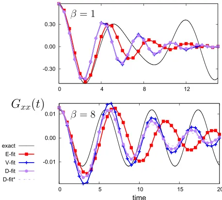
FIG. 2. Gxxfor low (β= 8,top panel) and high (β= 1,bottom panel)

tempera-tures for the mildly anharmonic model1 2x

2₊1 10x

3₊ 1 100x

4_{. Labels correspond}

to numerical derivatives for Eq.(23)explained in SubsectionIII B. The dashed line corresponds to not using the correction of Eq.(28). In black, we show the exact quantum mechanical results.

C. Anharmonic models at high and low temperatures

We tested the HPA-MC approximation for the anharmonic models given in Eq.(24), by computingGxx(t) andGx2_x2(t) cor-relation functions at high (β= 1) and low (β= 8) temperatures. We used the numerical interpolations described above, D-fit, V-fit, and the exact derivatives E-fit. To ensure a smallPsource error (see theAppendixfor more detailed discussion), we used a greater number of beads than that suggested by Eq.(A9). To use Eq.(A9), we took the effective harmonic force con-stant determined in the first step of the procedure described in Sec.III A[pertaining Eq.(26)], with a sufficiently converged number of beads.

FIG. 3. G_x2_x2 for low (β= 8,top panel) and high (β= 1,bottom panel) temperatures for the mildly anharmonic model 1₂x2+₁₀1x3+₁₀₀1 x4. Labels correspond to numerical derivatives for Eq.(23)explained in SubsectionIII B. The dashed plot corresponds to not using the correction of Eq.(28). In black, we show the exact quantum mechanical results.

FIG. 4. Gxxfor low (β= 8,bottom panel) and high (β= 1,top panel)

tempera-tures for the strongly anharmonic model1₄x4. Labels correspond to numerical derivatives for Eq.(23)explained in SubsectionIII B. D-fit* is the same as D-fit but using fixed number of beads throught,P= 60 (bottom panel). In black, we show the exact quantum mechanical results.

In Figs.2and3, we show the results forGxx(t) andGx2_x2(t) for the mildly anharmonic model at low and high tempera-tures. This model exhibits one of the main shortcomings of this approximation; for any potential with non-symmetric terms (i.e., ₁₀1x3), the correlation functions suffer from a monotonic growth in errors as a function oft, for any position correlation function [an analogous error also occurs forG_x2_x2(t) for the harmonic oscillator, which originates from the use of a small number of beads P (see the Appendix)]. In this case, how-ever, increasing the number of beads does not eliminate this problem. Instead, this error arises because the HPA-MC phase factorF, which is included in the calculation of correlation functions and expectation values here, is an approximation and so introduces an error. However, because we know the correct expectation values (from exact PIMD or PIMC simulations at real-time t = 0), we can approximately correct this error by a simple, albeitad hoc scaling. Specifically, because we know that expectation values should be independent of time, the following correction can be applied:

G∗_xx(t)=Gxx(t)

hx1i2(t=0)

hx1i2(t)

!

,

G∗

x2_x2(t)=Gx2_x2(t)* ,

hx2₁i2(t=0) hx2

1i2(t) +

-.

(28)

Sincehx1|2

1 iconverges quickly, this correction can be applied

with little additional cost. To ensure a minimal error arising from the number of beadsP, we used three times the suggested number by Eq.(A9). This resulted in 2P= 42 beads att= 0 and 2P= 128 att= 25.

of the fact that the harmonic interpolated approximation of the potential energy surface will become increasingly inac-curate at higher temperatures (loosening of ring beads). The results for the interpolated approximations without the scaling of Eq.(28)are also shown, demonstrating monotonic growth in the error associated with propagation of the error in the har-monic approximation at longer times. It is also worth noting that for the exact derivatives this error is not present at high temperatures (the scaling factor is nevertheless used for E-fit in Figs.2and3).

From the Gxx(t) results in the top panel of Fig. 2

(β = 8), one can observe that, although the phase matches the exact results, the correction re-scaling has the unfortunate effect of reducing the amplitude of the oscillations, making the approach only feasible for moderate times. E-fit exhibits a smaller amplitude but appears to decay slower than the interpolated approximations. On a similar note, the mono-tonic growth in the error for E-fit is present but smaller than for the other two approximations (the dashed line shown in Fig. 2 is using V/D-fit). For the interpolated approxi-mations, the problem is exacerbated further at high tem-peratures (bottom panel), with the amplitude decaying very rapidly when using the re-scaling of Eq.(28). In contrast, the exact derivative performs much better, with little decay over time.

Somewhat surprisingly, the interpolated approximations ofG_x2_x2(t) for low temperaturesβ= 8 [Fig.3with the correc-tion of Eq.(28)] do better at semiquantitatively maintaining the amplitude and phase to longer times. The exact derivative maintains the phase over the time shown, with an incorrect, smaller amplitude. The error growth is as severe as for the inter-polated approximations. The convergence of these TCFs is much tougher to achieve than their corresponding odd-termed correlation functions (as discussed in SubsectionIII D).

The behaviour of the exact and interpolated methods could perhaps be rationalised by considering three key points. First, for anharmonic models, the use of the HPA factorF(x+) in the calculation of the correlation function will introduce an error; this factor is derived based on assuming a harmonic potential and cannot account for anharmonic terms. Second, at low temperatures, when the region of phase-space explored by the ring-polymer is expected to be confined to regions near the bottom of the PES, the harmonic interpolation of the PES might be expected to be quite accurate, particularly for mildly anharmonic systems; as a result, the error introduced by the HPA would be expected to be smaller. Third, at high temper-atures (small β), the ring-polymer explores a larger degree of phase-space, including regions of significant anharmonic-ity; as a result, the HPA would be expected to become more inaccurate. Taken together, these comments suggest that inter-polation methods such as V-fit and D-fit should work better at low temperatures (large β), whereas the E-fit method should work better at high temperatures. This trend is evident in Figs.2and3.

For higher temperature, interpolated approximations (lower panel of Fig. 3), the scaling factor leads to an erro-neous decay which only mildly fixes the error growth. The amplitude and phase are also mostly lost by 25 reduced units of time. In contrast, the exact derivative gives much better

results over the time shown, with the scaling factor slightly improving the result. The fact that the interpolated approxima-tions seem to give TCFs which decay with time suggests that the harmonic factorF(x+) calculated using interpolation is simply not sufficiently accurate at higher temperatures, where significant anharmonicity will be encountered; in this case, the rescaling procedure seems to over-damp the TCFs. In contrast, the exact derivatives (E-fit) result in a good approximation to the exact TCF. In this case, presumably because the calculated factorF(x+) in some way incorporates some of the effects of anharmonicity via the use of exact derivatives.

Next, Fig. 4 shows Gxx(t) for the strongly anharmonic

model (i.e., the quartic oscillator). For all cases, both the amplitude and phase are lost by 20 units of time, and the error begins within the first period. For the low temperature regime (bottom panel of Fig. 4), in all three instances, the first period is over-shot, but the overall frequency-increase and amplitude-decay errors gradually grow as time increases. The potential-only V-fit shows an excessive amplitude at short times, which is improved by the gradient, D-fit, interpolation. Unfortunately this improvement in D-fit also means that the amplitude approaches zero faster. The exact derivative results, E-fit, exhibit a longer period of oscillation but suffer less amplitude-decay or a frequency-increase error. Despite these shortcomings, the numerical derivative approximations exhibit semi-quantitative results for three periods before decaying. In contrast, results in the high-temperature regime (β = 1, top panel of Fig. 4) are much worse, exhibiting errors in frequency and amplitude by the end of the first period of oscillation. All information is lost by 15 units of time. The exact derivatives perform somewhat better than the numerical derivative cases. Similar poor behaviour is observed in other methods, such as RPMD/CMD.83 _{The explanation given}58 in those methods is that long term oscillations on high tem-perature regimes arise from higher-order terms in the phase. Higher-order terms are also explicitly missing in this approx-imation. Since there is a qualitative resemblance between the poor performances of RPMD/CMD and HPA, these missing terms might also be the explanation here. We used four times the number of beads suggested by Eq.(A9). This resulted in 2P= 20 att= 0 and 2P= 124 att= 20. Nevertheless, more mod-est number of beads can be used to obtain similar results, with little decay of the amplitude. Converged results for 2P= 60 in dashes for D-fit in the low temperature panel in Fig.4show that the quality of interpolation is not significantly affected by such choice ofP. Nevertheless, a decrease in amplitude creeps in at slightly earlier times for smallerP, similar to the harmonic oscillator cases.

D. MC convergence

position and position-squared correlation functions as

δ(x1₁x_P+11 )=(hx₁2x2_P+1i − hx1xP+1i2)

1 2

and

δ(x2₁x2_P+1)=(hx₁4x_P+14 i − hx₁2x2_P+1i2)21

for the harmonic oscillator potential. The central limit theorem can approximately suggest the relative cost of convergence using an idealised Monte-Carlo integrator. For the system parameters 2P= 80,β= 8,t=π(time for whichhx1xP+1i2=0),

we get δ(x1 1x

1

P+1) ≈ 1 and δ(x 2 1x

2

P+1) ≈ 3, suggesting that it

would be more expensive by nearly a factor of three to reduce the error in the correlation function involvingx2 _{to the same}

value as the correlation function for justx. If a relatively small number of beads is chosen such that the monotonically increas-ing error due toPobserved forG_x2_x2(t) (Appendix) occurs at smallt, the central limit theorem suggests thatGxx(t) will also

become harder to converge, owing to the increase inδ(x1₁x_P+11 ) (which depends onhx2₁x_P+12 i).

However, the rough estimates above can underestimate drastically the cost of converginghx₁2x2_P+1isince the ideal vari-ance of the error should be at least an order of magnitude smaller than the characteristic amplitude of oscillations on hxn

1x n

P+1i. We note that the amplitude of oscillations inhx 2 1x2P+1i

have an inverse relationship to the frequencyω2, and so, if, for example, we usedω2 = 1 (β= 8), the amplitude of oscilla-tion observed forhx2₁x2_P+1i would be∼10−4, suggesting that we should converge the integral to∼O(10−5). For this reason, we choseω2=1₈ for the harmonic oscillator example studied here since one gets comparable magnitudes for the amplitude of oscillation forhxn

1x n

P+1i,n=1, 2 (n= 2 is shown in Fig.5).

The top panel in Fig.5shows a measure of cost of converge ε(nmc), as the difference between the converged correlation

functions ofGxn_xn,n = 1, 2, 3 and their values for different number of MC steps, across three orders of magnitude and averaged over 20 units of time. Here, we define

ε(nmc)=

1 Nt

Nt X

i

Gxn_xn(t_i)nmc−G_xn_xn(t_i)n∞

/σ¯n, (29)

where

¯ σn=

1 Nt

Nt X

i

Gxn_xn(t_i)n∞−G_xn_xn

(30)

and

Gxn_xn =

Nt X

i

Gxn_xn(t_i)n∞/N_t.

Here,ε(nmc) is the difference between the correlation function

Gxn_xn after n_mc Monte Carlo integration and the converged n∞ ≈ 109 result, averaged over Nt equidistant time slices

0≤ti≤20.ε(nmc) is also re-scaled by ¯σn, the standard

devi-ation of the oscilldevi-ations averaged over the same time domain so as to place the errors of these different correlation functions approximately on the same footing (this makes the scale in Fig.5 arbitrary). It is worth noting that converging all TCFs at high temperatures is considerably easier, the number of samples being cut by at least an order of magnitude.

There is a clear difference in cost betweenGxn_xn,n=1, 3 (blue cross and red filled square) andn= 2 (green circle). This

FIG. 5. (Top) Convergence of error [Eq.(29)] with respect to number of MC stepsnmcfor different correlation functions of the models tested (β= 8, 2P

= 80), see text for details.Legend: HO: Harmonic Oscillator; SA: Strong Anharmonic; MA: Mild Anharmonic. Also shown are three of the more costly correlation functions from the top panel at different number of MC steps:G_x2_x2 for1₈x2_{(second from top),G}

xxfor the strong (second from bottom), andGx2_x2 for the mildly (bottom) anharmonic models.

is partly due to the amplitude of oscillations being typically larger and can cross the y axis, so the coherence can be resolved “quicker.” This difference in amplitude was partially addressed by the ¯σn-rescaling just described. To exhibit approximately

the same relative error betweenn= 1 andn = 2, we require nearly two orders of magnitude number of samples. Despite this cost, with 106.5 _{steps, one is already able to minimise}

the error sufficiently to exhibit oscillations, as can be seen for the harmonic oscillator in the second from the top panel of Fig.5. The re-scaling for the monotonic error growth inG_x2_x2 described in Subsection1of the Appendix was used to get a better estimate of convergence using Eq.(29)(though for 2P = 80, it is only a small shift).

Also shown in Fig.5 is the convergence ofGxx for the

The rescaling by ¯σnin this case slightly exaggerates the cost it

takes to converge this correlation function, since the amplitude decreases towards zero as it approaches t = 20, leading to a larger error for “later” real-times. This can be seen in the second from the bottom panel of Fig. 5, which also shows the convergence for different number of MC steps; the “early” (t <10) times are clearly resolved compared to later ones by 106.5_{MC steps.}

Finally, the cost of convergence ofG_x1|2_x1|2for the mildly anharmonic model is also shown in Fig.5. ConvergingGxx(t)

(brown up triangle) has approximately the same cost as that for the strongly anharmonic model (orG_x2_x2(t) for the harmonic oscillator). The most expensive of all correlations evaluated was G_x2_x2 (sea green down triangle), for this mildly anhar-monic model, which took∼109.5samples to make it smooth (see the bottom panel). However, it is worth noting that despite the noise in the results, a clear coherence is observed by∼108, and maximum entropy analytic continuation (MEAC) tech-niques could then possibly be applied to this orG_x2_x2(t) to obtain a better approximation to the spectra.54,90

IV. DISCUSSION

The weighting function,F, gives importance to trajecto-ries near the classical path [Eq.(21)], and in this sense, it is reminiscent to stationary phase filtering methods85or includ-ing samplinclud-ing functions which weight away from highly oscil-latory regions.30,84In fact, the first and most obvious way one would think to useF(x+) would precisely be as an importance sampling function to weigh the sampled regions near the clas-sical path, as shown in Eq.(21). However, our experiments in this direction to date [in other words, usingF(x+) as an addi-tional importance sampling function with which to calculate GAB(t) using Eq.(3)] have not been successful. In particular,

we find that using F(x+_{) as an importance-sampling}

func-tion fails to improve sampling in Eq.(3). The functionF(x+₎

only depends on the coordinates of the central “sum” string, while the dependence on the difference coordinates appears implicitly via the harmonic approximation of the PES. As a result, this importance sampling of the difference coordinates does not do enough to sufficiently alleviate the “sign problem” which appears in any scheme for calculating properties using Eq.(3).

The HPA-MC method, as proposed here, seems to suf-fer from inaccuracies at all times for anharmonic potential. These same symptoms are worst for the high temperature case (β= 1), where coherences are observed, but with the wrong frequencies for longer times, a problem which is also appar-ent in other standard methods.22,58_{For anharmonic potential} containing odd terms, it was necessary to include a re-scaling factor in order to avoid a monotonic growth in the error for the position correlation functions. This also leads to a rapid decay of the Gxx autocorrelation function which makes the

method inapplicable to study long time dynamics. The evalu-ation ofG_x2_x2proved to be particularly costly, suggesting that better sampling techniques would be required if one desired to apply this approach to larger systems. Conceivably, the use of maximum entropy analytic continuation (MEAC) meth-ods could improve the frequency-domain inversion required

to obtain the spectra of the dynamical operator in question from this approximation.82,90,91The poor performance at high temperatures and long times can be in part traced to the loos-ening of the bead spring terms _4|mP_τ|2β

~2, which lead to a larger

distances between of the forward and backward beads x, x0

for which sum/difference coordinates are used. The harmonic interpolation of the potential for large |x−x|0 _{leads to a}

poorer estimation of the contribution of the phase to the TCF integral.

Equation(22)shows that integrating over the mixed tem-perature (imaginary time) and real time leads to a classi-cal evolution which has a “memory” of the trajectory tra-versed, via the coupling matrix ((H−)−1_ij ), the covariance of the displacements along the difference coordinates. How-ever, it is worth noting that the elements ((H−)−1_iP), 2 ≤ i ≤ P decay rapidly as P i increases, suggesting a limit to how the more distant evolution of x+ beads affect the x+

P+1bead. Developing approximations utilising this insight,

together with the fact HPA-MC work for short times, are being investigated.

Further serious issues are likely to arise for systems whose potential exhibits points with negative curvature, such as tran-sition state barriers, or PESs, such as the Morse function; in such cases, the Fourier transform along the difference coordi-nates is no longer well defined, and the expression in Eq.(19) [or(23)] would result in a poor representation of the integral. As a first approximation, it would be conceivable to set any negative curvatures present to zero and treat the coordinate as a free particle in such regions. It is also worth noting that similar problems arise in methods which rely on harmonic approx-imation of the PES in order to sample the thermal Wigner distribution.76_{In such cases, Miller and co-workers have} pro-posed methods to approximately correct this by replacing imaginary eigenvalues with appropriate positive eigenvalues. We hope that such similar approaches might also be applica-ble in the context of HPA-MC, and work is ongoing in this direction.

higher-order PIMD simulations. Again, these issues remain for future work.

Despite the reasonable performance exhibited for 1D model problems at low temperatures, it remains to be seen whether this approach will work effectively with a larger number of degrees of freedom, as well as for systems cou-pled to some environment. A second-order expansion of a multi-dimensional potential with coupling terms would result in cross terms in the system Hessian. Such terms could be, for example, approximated by the numerical partial sec-ond derivatives from the ρ-sampled geometries. Similarly, a many-coordinate generalisation for obtaining temperature-dependent effective frequencies as described in Subsection III A, which one uses to generate a harmonic-phase normal representation is likely possible.

The principal bottleneck in the evaluation ofFcan be narrowed to calculate (H)1[the generalisation of Eq.(A3)]. We therefore expect the cost of the algorithm to scale at most as O(n3_{)} withn = PN, whereN is the number of system}

degrees of freedom.Hcan be shown to be no longer tridiag-onal but can take a quasi-block diagtridiag-onal (banded) form. The cost of invertingHwould amount to the cost of inverting such blocks and the sparse matrix multiplication involving these,94 thereby reducing the cost of matrix inversion. This method is more expensive than (linear-scaling) semiclassical methods that compute correlation functions, which only require clas-sical trajectories sampling an initial distribution over phase-space. But, it will nevertheless be worth investigating how robust this approach is when applied to real problems.

V. CONCLUSIONS

From the standard position path-integral form of the sym-metric complex correlation function, we employed the well-known sum/difference transformation between the beads in the forward and backward paths and introduced a harmonic approximation for the potential energy surface, resulting in a Gaussian weighting which can be used to approximately recover the coherence between the forward-backward paths. HPA-MC was used to study 1D model problems typically used in the literature. The correlation functions for harmonic sys-tems are exact. Appealingly, it can in principle also provide time-correlation functions for non-linear operators, which can be required for the evaluation of a number of dynamical quan-tities,95 _{such as measured, for example, incoherent dynamic} structure factors during inelastic neutron scattering.65 _The method provides a reasonable approximation of linear and non-linear operator TCFs for anharmonic models, for short times and low temperatures, and should also be easily implemented in MD programs. The approximation is likely to maintain zero-point energies and could be easily applied to represent

many-electron degrees of freedom. Despite these advantages, the approximation is unable to provide information for long real-times and high temperatures for anything other than har-monic oscillators. Nevertheless, it is the authors’ hope that despite these shortcomings, the ideas presented here may lead to further approximations and algorithms that may overcome these limitations, some of which are currently underway.

ACKNOWLEDGMENTS

The authors gratefully acknowledge funding for this project by the Leverhulme Trust (No. RPG-2016-003). Computational resources were provided by the Scientific Computing Research Technology Platform at the Univer-sity of Warwick. Data from Figs. 2–8 can be found at http://wrap.warwick.ac.uk/id/eprint/91744.

APPENDIX: ANALYSIS OF HPA-MC TCF FOR HARMONIC PESs

For a harmonic oscillator, the system potential separates the sum/difference coordinates exactly, and the x1 andxP+1

coordinates are only coupled to thex+ coordinates in ρ+. If one wishes to evaluate the density∫ dxˆρ, one needs only to sample theρ+part, which contains onlyP+ 2x+coordinates, as opposed to 2P. For TCF of operators involving purelyx1,

xP+1beads ρ+ is a more succinct representation of the

den-sity, and all contribution from the phase arise from the integral ∫ dq−ρ−eiΦ0=F−, which depends solely on thex+coordinates and its derivatives. This observation motivated the HPA-MC approximation used in this article. For the harmonic oscilla-tor model, the exponent in ρ+F is quadratic inx+_{, and the}

Hessian can be evaluated for once and for allt. We shall ana-lyze the dependency correlation functions have on the systems variablesβ,t,m,P, andω.

In what follows, we shall seta =1/√2 so that all repre-sentations shown below will be related via rotations to the Cartesian coordinates. Though not immediately relevant to MC algorithms, this choice has some implications when con-sidering MD methods of integration, and in particular, when considering how to provide “appropriate” masses to the kinetic energy of beads. Any choice other thana =1/

√

2 makes the new coordinates unevenly stretch/compress the relative areas of thex,x0in phase-space. This results in the effective masses of the KE operator to be different to those ofx+₁andx_P+1+ (only labelled with + for convenience) and rotating to a diagonal Hessian (normal mode) representation from these scaled coor-dinates would lead to a non-diagonal KE operator.83_Labelling the rotation representation a = √1

2 as x √

, to transform to it

from any other choice ofa, we must scale byx

√

+_=a√_2x+_and

x

√ −₌√

2/2ax−. Define vector~dkin the basis ofx+coordinates

~_d

k= P+1

X

i=1

dkixk+, dki=         

2, i=k −α, i=k−1 −γ, i=k+ 1 0, |i−k|>1

,

α=(1/a, i=1

1, i>1, γ=(1/a, i=P+ 1

1, i<P+ 1,

This vector can then simplify the expression in Eq.(19), so the variables in the exponent of ln(F−)=ϕ[Eq.(19)] are then

P

X

k=2

(C_k+)2 (λ−

k)2+ (

τω

P )2

=

P

X

k=2

(PP i=2U

− ki

PP+1

α=1(diα−(

τω

P ) 2_δ

iα)x+α)2

(λ− k)2+ (

τω

P )2

=

P+1

X

α,γ=1 P

X

i,j=2

x_γ+(diγ−( τω

P )

2_δ iγ)(

P

X

k=2

U− kiU

− kj

(λ−_k)2_{+ (}τω P )2

)(djα−( τω

P )

2_δ

jα)x+α, (A2)

whereϕcan be broken into the sum of three matrices,

ϕ=mt_τ22_βP(x+)T_D−

(τω P )

2_F

+ (τω P )

4_H−1 _x+

,

Dij =( P

X

k,l=2

dki(H−)−1kl dlj),

Fij=( P

X

k,l=2

dki, (H−)−1_klδlj+δki(H−)−1_kldlj)

(H−)−1_kl =

P

X

i=2

U_ik−U_il−

(λ−_i)2_{+ (}~τω

P )2

.

(A3)

The eigenvalues of these also depend on P via the dimen-sions of thexbeads,P1. All three matrices depend on all system parameter viaH, the inverse of which can be shown to have analytic solutions.96 _{Therefore, the problem has, in} principle, an analytic solution. We shall here restrict ourselves to solutions via linear algebra; we can find the eigenvector

representation which diagonalises both the Gaussian density and phases,

1 2(x

+

)TRTR( βmP 2~2τ2

H++ 2ϕ)RTRx+=1 2r

T_Λr

,

Λ_ii=λϕ+ i =

P+1

X

α,γ=1

mPβ 2~2τ2(

RγiHγα+ Rαi)

(A4)

+2mPt

2

β_~2τ2

Rγi

Dγα−(τω P )

2_F

γα+ (τω P )

4

(H−)−1γα

Rαi

.

We defined the formally positive semidefinite λϕ_i+without a square to simplify notations.

1. Position correlation functions

To keep the problem tractable, we shall restrict ourselves to studying the position autocorrelation functionA=B=xn_.

From Eq.(A4), we can write down the correlation functions Gxn_xn, to different ordersn:

Gxx=he−ϕρ+i−1

dr(

P+1

X

i,j=1

R1iriR(P+1)jrj)e− PP+1

k=1λ

ϕ+ k r

2 k/2=

P+1

X

i=1

R1iR(P+1)i λϕ+

i

,

G_x2_x2 =he−ϕρ+i−1

dr(

P+1

X

i,j,k,l=1

R1iriR1jrjR(P+1)krkR(P+1)lrl)e− PP+1

k=1λ

ϕ+ k r

2 k/2

=

P+1

X

i,j=1

(R2_1iR2_(P+1)j+ 2R1iR(P+1)iR1jR(P+1)j)(λϕ_i+λϕ_j+)−1,

G_x3_x3=

P+1

X

i,j,k=1

(9R2_1iR2_(P+1)i(R1kR(P+1)k) + 6(R1iR(P+1)i)(R1jR(P+1)j)(R1kR(P+1)k))(λϕ_i+λϕ_j+λϕ_k+)−1,

G_x4_x4 =

P+1

X

i,j,k,l (

9R2_1iR2_1jR2_(P+1)kR2_(P+1)l+ 56R2_1iR2_(P+1)j(R1kR(P+1)k)(R1lR(P+1)l)

+ 24(R1iR(P+1)i)(R1jR(P+1)j)(R1kR(P+1)k)(R1lR(P+1)l) )

(λϕ_i+λϕ_j+λ_kϕ+λϕ_l+)−1,

(A5)

wherehe−ϕ_ρ+_{i =} QP+1

i=1

q_2π λϕ+

i

. Figure6 shows sixteen

dis-tributions corresponding tohe−ϕ_ρ+_{ifor different values ofP}

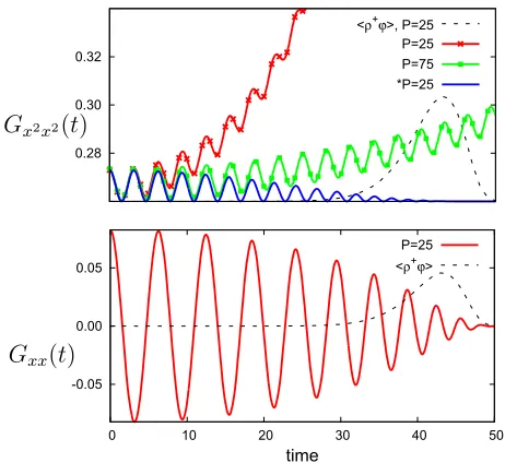
along 10<t <140. Each distribution has been normalised to emphasize the linear relationship between the maxima of the distribution andP(discussed in Subsection2of the Appendix). The right-hand tail of each distribution drops sharply to zero and determines how far intthe expectation value of any oper-ator can be estimated. Figure7shows a representative case of how Gxx andGx2_x2 behave as a function oft for β= 5,ω2 = 1,P= 25. The amplitude ofGxxgradually decreases as it

reaches the right-hand tail of he−ϕρ+i(lower panel), shown in black dashes and scaled. The oscillations inG_x2_x2 (upper panel in Fig.7) also decrease, but worse, it very quickly suffers from a severe non-oscillatory monotonic growth astincreases (see red,P = 25). The spectra obtained resulting from such errors is likely to be poor. This symptom can be obviously addressed by increasingP, as shown in theP= 75 case, but it does suggest that to obtain a good estimate, one might need approximately four times more beads than forGxx.