Research of correlation between electric soil conductivity and yield based on the use of GPS technology

Efficient and accurate methods of measuring with-in-field variations in soil properties are important for precision agriculture (Bullock & Bullock 2000). The apparent profile soil electrical conductivity is one sensor-based measurement that can provide an indirect indicator of the important soil physical and chemical properties.

Soil salinity, clay content, cation exchange capacity (CEC), clay mineralogy, soil pore size and distribu-tion, soil moisture content, and temperature all af-fect EC (McNeill 1992; Rhoades et al. 1999).

In saline soil most of the variations in EC can be re-lated to the salt concentration (Williams & Baker 1982). In non saline soils, conductivity variations are primarily a function of soil texture, moisture con-tent, and CEC (Rhoades et al. 1976; Kachanoski et al. 1988). Rhoades et al. (1989) modeled EC as a function of soil water content (both the mobile and the immobile fractions), the electrical conductivity (EC) of the soil water, soil bulk density, and EC of the soil solid phase.

The measurements of EC can be used for providing indirect measures of the soil properties listed above if

the contributions of other soil properties affecting the EC measurement are known or can be estimated. If the EC changes due to one soil property are much greater than those attributable to other factors, then EC can be calibrated as a direct measurement of that dominant factor. Lesch et al. (1995a, b) used this direct-calibra-tion approach to quantify the variadirect-calibra-tions in soil salinity in a field where the water content, bulk density, and other soil properties were reasonably homogeneous.

The mapped EC measurements were found to be related to a number of soil properties of interest in precision agriculture, including soil water content (Sheets & Hendrickx 1995), clay content (Wil-liams & Hoey 1987), CEC, and exchangeable Ca and Mg (McBride et al. 1990). Because EC inte-grates texture and moisture availability, two soil characteristics that affect productivity, it can help to interpret spatial grain yield variations, at least in certain soils (Jaynes et al. 1993; Sudduth et al. 1995; Kitchen et al. 1999). Other uses of EC in precision agriculture include refining the boundaries of the soil map units and creating subfield manage-ment zones (Fraisse et al. 2001).

Partly supported by the Czech University of Life Sciences in Prague, Project No. IGA 31180/1312/313145/2004to improve the measuring equipment even second for purchasing measured data of crop yield number: FRVS 31180/1161/311602.

Research of correlation between electric soil conductivity

and yield based on the use of GPS technology

L. Ryšan, O. Šařec

Faculty of Engineering, Czech University of Life Sciences in Prague, Prague, Czech Republic

Abstract: A contact method was used for the continuous measuring of soil electric conductivity using a six disc electrodes apparatus. The placement of the electrodes was chosen on the basis of the depth of the profiles surveyed: 0–0.3 and 0–0.9 m. Two Crop Research Institute fields and two private Farma Dolejšová fields were followed in 2004 and 2005. For the treatment of the EC data obtained and of other information, the tools of geostatistic were applied. Arc View GIS software and its module Geostatistical analyst were used for the analysis of the geo-data obtained and for the elaboration of the soil conductivity and crop yield maps. Four variogram models were tested. Geostatistical analyses make relatively rigorous demands on wide-sense stationarity or at least average stationarity. The selection of any one of the four geostatistical variogram models did not affect the final maps. Exponential model is recommended. The experimentsdocumented a correlation between the two EC profiles investigated but no correlation was found between EC and the yield of crop. Every field and every property has its own characteristic surface which does not correspond with other ones.

MATERIAL AND METHODS

A contact method was used for the continuous measuring of soil electric conductivity. This type of method uses electrodes, usually in the shape of coulters, that make a contact with the soil to measure the electrical conductivity.

It was preceded by an apparatus with six disc elec-trodes (Figures 1, 2). This equipment is designed to join with the tractor three-point hanger, so that its sensors – circular electrodes – may be in an uninter-rupted contact with soil. The placement of electrodes was chosen on the basis of the depth of the profiles surveyed: 0–0.3 and 0–0.9 m. In this approach, two to

three pairs of coulters are mounted on a tool bar; one pair applies electrical current into the soil while the other two pairs of coulters measure the voltage drop between them. The soil EC information is recorded in a data logger along with GPS location information.

The resistivity meter involves applying a voltage into the ground through metal electrodes and mea-suring the resistance to the flow of the electric cur-rent. An AC-power source supplies current flow (I) between the two outer electrodes and the resultant voltage difference (V) between the two inner elec-trodes is measured.

The resistance of the soil is given by R = V/I. This needs to be standardized over the unit length. The

Figure 1. Scheme of coulter-electrodes Milsom (1989)

Figure 3. EC semivariograms – k Hostivici (14. 4. 2004, profile 0.3 m)

Figure 2. Measuring equipment constructed by Department of Machinery Utilization, Faculty of Engineering

(γ/102_{) (γ/10}2₎

(γ/102_{) (γ/10}2₎

Distance (h/102_{) Distance (h/10}2₎

resistance multiplied by the length (of the resistor in this case the soil) is called the resistivity (r) which is measured in ohm.m. The equation is:

r = 2πd R = 2πdV/I

where:

d – the spacing between the electrodes (m)

Alternatively, this can be expressed in terms of conductance (C = 1/R, Ω–1 _{= S) and conductivity}

(c = 1/r, Ω–1_{/m = S/m). The equation for the (soil}

electrical) conductivity (EC) is given by: c = 1/(2. πdR) = I/(2. πdV) _(S/m).

Electrodes have been replaced by rotating discs which are placed directly into the soil. As the cart

Table 1. Measured and analysed EC data – Crop Research Institute

Date

Field

"k Hostivici" (16 ha) "u Mostu" (12 ha)

profile (m) 0.3 0.9 0.3 0.9

14. 4. 2004

rows of data 1 118 1 118 771 771 minimum (mS/m) 43.963 20.473 30.894 17.151 maximum (mS/m) 132.63 83.032 126.22 64.946 delta max–min 88.667 62.559 95.326 47.795 average 75.167 49.828 54.417 37.364 stand. error 13.408 10.303 13.476 8.676 median 73.687 50.131 51.532 36.925 scewness 0.79207 –0.15408 2.116 0.3469 kurtosis 4.3035 2.9709 9.488 2.774

1. 9. 2004

rows of data 1 363 1 363 928 928 minimum (mS/m) 14.062 6.043 33.664 6.806 maximum (mS/m) 125.26 35.752 176.73 42.969 delta max–min 111.198 29.709 143.066 36.163 average 66.778 21.022 87.079 20.136 stand. error 18.501 4.55 27.487 5.3178 median 67.711 21.169 79.724 19.448 scewness –0.0891 -0.0505 0.5852 0.6899 kurtosis 2.8994 2.9269 2.6269 4.376

7. 9. 2005

rows of data 623 623 446 446

minimum (mS/m) 0.858 0.36487 0.813 0.30065 maximum (mS/m) 90.666 31.904 223.14 24.626 delta max–min 89.808 31.53913 222.327 24.32535 average 15.494 8.266 63.85 7.325 stand. error 14.761 6.842 67.172 5.9094 median 10.391 6.338 18.079 6.123 scewness 1.7567 0.9211 0.496 0.70284 kurtosis 6.8891 3.0101 1.4996 2.6749

Table 2. Analysed yield data (16. 8. 2004) – Crop Research Institute

Field "k Hostivici"

is pulled through the field, one pair of electrodes passes electrical current into the soil, while two other pairs of electrodes measure the voltage drop.

The data of corn yields were obtained from the owners with no information about raw data measur-ing or analysmeasur-ing.

Investigated fields

The data were collected from two Crop Research In-stitute fields and two private Farma Dolejšová fields. Crop Research Institute (CRI) fields: "k Hostivici"

– 16 ha, "u Mostu" – 12 ha

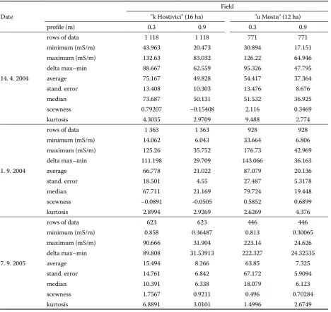
Figure 4. EC maps – b o t h p r o f i l e s – k Hostivici (14. 4. 2004)

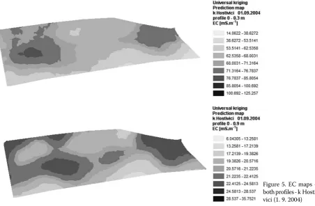
Figure 6. EC maps – both profiles – u Mostu (14. 4. 2004)

Dolejšová fields: "Dlouhé" – 8.73 ha, "u Háje" – 13.65 ha.

The measured and analysed EC data from the Crop Research Institute fields are shown in Table 1, while Table 2 shows the measured and analysed data of the crop yield.

The data were measured once during the spring of 2004 and twice in the autumn of 2004 and 2005. The soil moisture conditions were relatively dry at the time of the data collection in both sites in the autumn. Due to this fact the measuring process was not going well as lots of rows (data sentences) went out. The situation is more favourable in springs be-cause a lot of winter water is present in the soil.

ArcView GIS software and its module Geosta-tistical analyst were used to analyse the geo-data measured and to create the soil electric conductivity and crop yield maps. Four variogram models were tested to this aim. Semivariograms of each model are show in Figure 3.

Figure 3 shows the variograms of four models which were used. The variogram shows the relations between the distance and the values of two adjacent places measured. Similarly, all pictures demonstrate

that no significant differences can be recognised. The same conclusion may be made with every analysed data for both profiles of EC and even the crop yield. It is recommended to use the most widely used ex-ponential variogram models.

The EC maps of k Hostivici field, 0.3 m profile on the left side, 0.9 m profile on the right side, are shown in Figures 4 and 5.

The EC maps of u Mostu field, 0.3 m profile on the left side, 0.9 m profile on the right side, are shown in Figures 6 and 7.

The simplest and fastest way to interpret a soil EC map is to compare it visually to the yield or soil sur-vey maps of the same field. A more rigorous analysis would involve rasterisation of the EC data and yield monitor data into square grid cells that are consistent with each other. The average EC values from the grid cells can be compared to the yield values from the corresponding cells using linear regression and other statistical techniques.

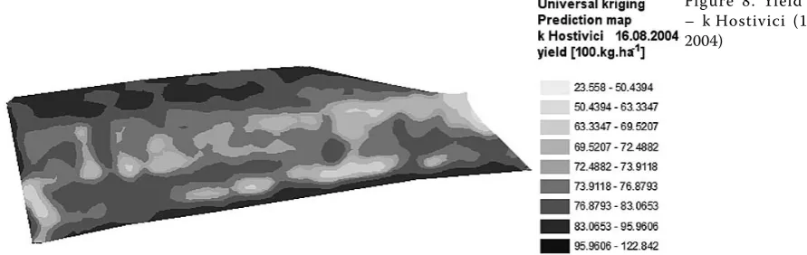
The grop yield maps of both fields in CRI are shown in Figures 8 and 9.

At first sight, it is easy to see that the maps of both profiles of EC data are similar even through the year

Figure 8. Yield map – k Hostivici (16. 8. 2004)

and in both fields as well. But no surface similarity between the EC and yields maps was recognised in either field.

The measured and analysed EC data from Dolejšová fields are shown in Table 3 while Table 4 shows the measured and analysed data of the crop yield.

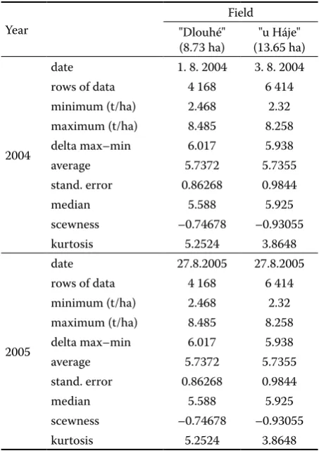
The EC maps of Dlouhé field, 0.3 m profile on the left side, 0.9 m profile on the right side, are shown in Figures 10 and 11.

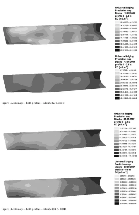
The crop yield maps from years 2004 and 2005 of Dlouhé field are shown in Figure 12.

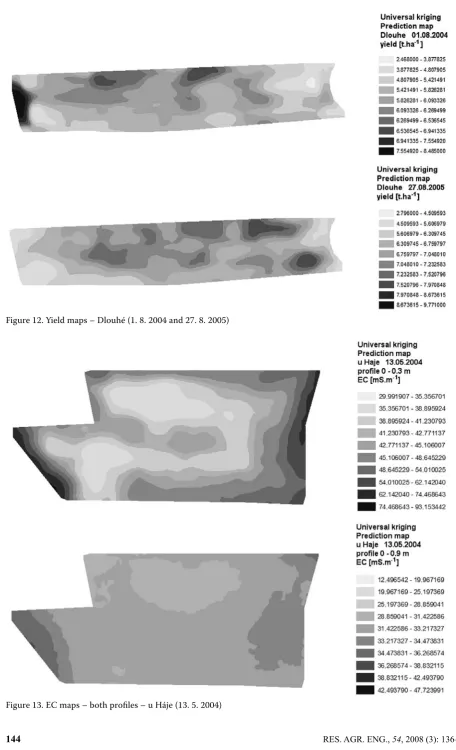
The EC maps of u Háje field, 0.3 m profile on the left side, 0.9 m profile on the right side follows (Figures 13, 14).

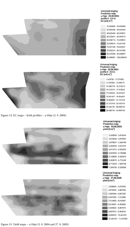
The crop yield maps from 2004 and 2005 of u Háje field are shown in Figure 15.

There are some facts shown by Dolejšová maps like those on CRI fields the maps of EC data from both profiles are rather similar, no matter if the data were obtained in spring or in autumn. Maximums and minimums are in the same places (have the same locations). But they are rather different from the yield maps. No correlation exists between the EC and the crop yield maps.

More sophisticated statistical methods are avail-able to evaluate the spatial and mathematical

simi-Table 3. Measured and analysed EC data – Dolejšová

Date

Field

"Dlouhé" (8.73 ha) "u Háje" (13.65 ha)

profile (m) 0.3 0.9 0.3 0.9

13. 5. 2004

rows of data 721 721 837 837

minimum (mS/m) 29.95 8.7127 29.992 12.497 maximum (mS/m) 83.192 59.097 93.153 47.724 delta max–min 53.242 50.3843 63.161 35.227 average 45.598 33.915 46.978 32.367 stand. error 8.1203 5.9761 9.9583 4.2221 median 44.123 32.895 44.941 31.924 scewness 1.0356 1.0799 1.511 0.29038 kurtosis 4.5686 6.4636 5.8181 4.9793

2. 9. 2004

rows of data 948 948 1 302 1 302 minimum (mS/m) 13.921 5.6139 16.364 7.4248 maximum (mS/m) 117.11 32.669 108.64 34.8 delta max–min 103.189 27.0551 92.276 27.3752 average 59.905 17.554 65.451 19.73 stand. error 17.268 4.0215 11.913 3.6825 median 58.155 17.2 66.019 19.315 scewness 0.3566 0.44711 –0.3361 0.6431 kurtosis 3.5015 3.691 4.3904 4.3968

Table 4. Analysed yield data – Dolejšová

Year

Field "Dlouhé"

(8.73 ha) (13.65 ha)"u Háje"

2004

date 1. 8. 2004 3. 8. 2004 rows of data 4 168 6 414 minimum (t/ha) 2.468 2.32 maximum (t/ha) 8.485 8.258 delta max–min 6.017 5.938 average 5.7372 5.7355 stand. error 0.86268 0.9844 median 5.588 5.925 scewness –0.74678 –0.93055 kurtosis 5.2524 3.8648

2005

Figure 10. EC maps – both profiles – Dlouhé (2. 9. 2004)

Figure 12. Yield maps – Dlouhé (1. 8. 2004 and 27. 8. 2005)

Figure 14. EC maps – both profiles – u Háje (2. 9. 2004)

larities between different layers including multivari-ate clustering (Lark et al. 1997), multifractal and autoregressive state-space analysis (Wendroth et al. 1999). These techniques are current research tools that may be included in future generations of precision farming software and crop simulation models.

DISCUSSION

The utility of EC mapping comes from the relation-ships that frequently exist between EC and a variety of other soil properties that are highly related to the crop productivity. These include such properties as water holding capacity (dry soil conductivity is much lower than that of moist soil), topsoil depth, soil nutrient levels and cation exchange capacity (CEC – presence of Ca, Mg, K, Na in the moisture-filled soil pores will enhance soil EC in the same way as salinity does), salinity (increasing concentrations of electrolytes (salts) in soil water will dramatically increase soil EC), soil drainage, organic matter level, and subsoil characteristics.

Using the soil electric conductivity measuring technology will differ from grower to grower and from region to region due to the differences in the soil characteristics, growers’ needs and interests, and users’ expertise in utilising the spatial data. For some uses, the grower or data analyst will need the access to a moderately powerful GIS rather than just simple yield mapping software. Private consultants and mapping centers will be needed to assist with EC mapping and analysis.

SUMMARY AND CONCLUSIONS

In this paper, the following conclusions are pre-sented. Soil EC has no direct effect on the crop yield. The experimentsdocumented no correlations between EC_SH and the crop yield even if the soil properties were indicative of productivity.

The actual conclusions confirmed a correlation between the surveyed profiles of 0.3 m and 0.9 m followed during springs and autumns as well as over the years. A certain relation can be found between the higher values of electric soil conductivity, low pH factors, and the high levels of groundwater present in the field. On the contrary the correlation between conductivity and plant yields was not unconfirmed. It is recommended to continue in the research of EC measuring and in the collection of data on soil properties, and to look for mutual relations and correlations.

References

Bullock D.S., Bullock D.G. (2000). Economic optimality of input application rates in precision farming. Precision Agriculture, 2: 71–101.

Fraisse C.W., Sudduth K.A., Kitchen N.R. (2001): Deline-ation of site-specific management zones by unsupervised classification of topographic attributes and soil electrical conductivity. ASAE, 44: 155–166.

Jaynes D.B., Colvin T.S., Ambuel J. (1993): Soil type and crop yield determinations from ground conductivity sur-veys. ASAE Paper No. 933552, ASAE, St. Joseph.

Kachanoski R.G., Gregorich E.G., Van Wesenbeeck I.J. (1988): Estimating spatial variations of soil water content using non contacting electromagnetic inductive methods. Canadian Journal of Soil Sciences, 68: 715–722.

Kitchen N.R., Sudduth K.A., Drummond S.T. (1999): Soil electrical conductivity as a crop productivity measure for claypan soils. Journal of Production Agriculture, 12: 607–617.

Lark R.M., Stafford J.V., From M.A. (1997): Exploratory analysis of yield maps of combinable crops. In: Stafford J.V. (ed.): Proc. 1st _{European Conf. on Precision Agriculture,}

Silsoe Research Institute, Silsoe, 887–894.

Lesch S.M., Strauss D.J., Rhoades J.D. (1995a): Spatial prediction of soil salinity using electromagnetic induction techniques: I. Statistical prediction models: A comparison of multiple linear regression and cokriging. Water Re-sources Research, 31: 373–386.

Lesch S.M., Strauss D.J., Rhoades J.D. (1995b): Spatial prediction of soil salinity using electromagnetic induction techniques: II. An efficient spatial sampling algorithm suit-able for multiple linear regression model identification and estimation. Water Resources Research, 31: 387–398. McBride R.A., Gordon A.M., Shrive S.C. (1990):

Esti-mating forest soil quality from terrain measurements of apparent electrical conductivity. Soil Science Society of America Journal, 54: 290–293.

McNeill J.D. (1992): Rapid accurate mapping of soil salin-ity by electromagnetic ground conductivsalin-ity meters. In: Advances in Measurement of Soil Physical Properties: Bringing Theory into Practice. SSSA Special Publication 30, SSSA, Madison, 209–229.

Rhoades J.D., Raats P.A., Prather R.J. (1976): Effects of liquid phase electrical conductivity, water content, and surface conductivity on bulk soil electrical conductivity. Soil Science Society of America Journal, 40: 651–655. Rhoades J.D., Manteghi N.A., Shrouse P.J., Alves W.J.

(1989): Soil electrical conductivity and soil salinity: New formulations and calibrations. Soil Science Society of America Journal, 53: 433–439.

D.L. (ed.): Assessment of Non-point Source Pollution in the Vadose Zone. Geophysical Monogr. 108, American Geophysical Union, Washington, 197–215.

Sheets K.R., Hendrickx J.M.H. (1995): Non invasive soil water content measurement using electromagnetic induc-tion. Water Resources Research, 31: 2401–2409.

Sudduth K.A., Kitchen N.R., Hughes D.F., Drummond S.T. (1995): Electromagnetic induction sensing as an indicator of productivity on claypan soils. In: Robert P.C., Rust R.H., Larson W.E. (eds): Site Specific Management for Agri-cultural Systems. Proc. 2nd _{Int. Conf., March 27–30, 1994,}

Minneapolis, ASA, CSSA, and SSSA, Madison, 671–681. Wendroth O., Jurschik P., Nielsen D.R. (1999): Spatial

crop yield prediction from soil and land surface state

variables using an autoregressive state-space approach. In: Stafford J.V. (ed.): Precision Agriculture ’99. Proc. 2nd

European Conf. Precision Agriculture, 419–428.

Williams B.G., Baker G.C. (1982): An electromagnetic induction technique for reconnaissance surveys of soil salinity hazards. Australian Journal of Soil Research, 20: 107–118.

Williams B.G., Hoey D. (1987): The use of electromagnetic induction to detect the spatial variability of the salt and clay content of soils. Australian Journal of Soil Research,

25: 21–27.

Received for publication August 23, 2007 Accepted after corrections December 11, 2007

Corresponding author:

Ing. Ladislav Ryšan, Česká zemědělská univerzita, Technická fakulta, Kamýcká 129, 165 21 Praha 6-Suchdol, Česká republika

tel.: + 420 461 618 000, fax: + 420 234 381 828, e-mail: [email protected]

Abstrakt

Ryšan L., Šařec O. (2008): Výzkum korelace mezi vodivostí půdy a výnosem s využitím technologie GPS.

Res. Agr. Eng., 54: 136–147.

Pro měření elektrické vodivosti půdy byla použita kontaktní metoda – šesti kotoučový měřící přístroj. Rozmístění elektrod bylo zvoleno podle požadované hloubky zkoumaných profilů: 0,3 m a 0,9 m. Měření probíhala v letech 2004 a 2005 na dvou pozemcích VÚRV Praha-Ruzyně a taktéž dvou pozemcích na soukromé farmě Dolejšová. Pro analý-zu a následné zpracování geo-dat a vytvoření map elektrické vodivosti a výnosu byly použity nástroje ArcView GIS a doplňující modul Geostatistical analyst. Relativně přísnou podmínkou pro použití geostatistických analýz je pod-mínka stacionarity respektive stacionarity druhého řádu. Rozdíly mezi použitím čtyřmi různých modelů variogramů se neprokázaly, zvolené modely neměly zásadní vliv na výsledné mapy. Doporučeno je používání exponenciálního modelu variogramu. Experimenty potvrdily jistý vztah mezi hodnotami EC a oběma zkoumanými profily, naopak se neprokázala korelace mezi elektrickou vodivostí půdy a výnosem. Vytvořené mapy ozřejmily přítomnost charakte-ristického rysu každého pozemku u všech zkoumaných vlastností, tyto charakteristické rysy jsou pro každý pozemek a každou vlastnost jedinečné.