An Introduction to
Statistical Signal Processing
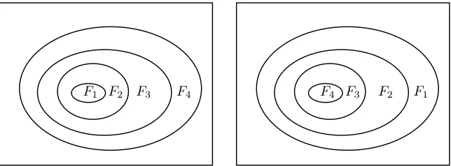
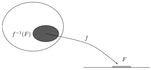
Pr(f ∈F) =P({ω:ω∈F}) =P(f−1(F)) f−1(F)
f
F
✲
An Introduction to
Statistical Signal Processing
Robert M. Gray
and
Lee D. Davisson
Information Systems Laboratory
Department of Electrical Engineering
Stanford University
and
c
Contents
Preface xi
Glossary xv
1 Introduction 1
2 Probability 11
2.1 Introduction . . . 11
2.2 Spinning Pointers and Flipping Coins . . . 15
2.3 Probability Spaces . . . 23
2.3.1 Sample Spaces . . . 28
2.3.2 Event Spaces . . . 31
2.3.3 Probability Measures . . . 42
2.4 Discrete Probability Spaces . . . 45
2.5 Continuous Probability Spaces . . . 56
2.6 Independence . . . 70
2.7 Elementary Conditional Probability . . . 71
2.8 Problems . . . 75
3 Random Objects 85 3.1 Introduction . . . 85
3.1.1 Random Variables . . . 85
3.1.2 Random Vectors . . . 89
3.1.3 Random Processes . . . 93
3.2 Random Variables . . . 95
3.3 Distributions of Random Variables . . . 104
3.3.1 Distributions . . . 104
3.3.2 Mixture Distributions . . . 108
3.3.3 Derived Distributions . . . 111
3.4 Random Vectors and Random Processes . . . 115
3.5.1 Multidimensional Events . . . 118
3.5.2 Multidimensional Probability Functions . . . 119
3.5.3 Consistency of Joint and Marginal Distributions . . 120
3.6 Independent Random Variables . . . 127
3.6.1 IID Random Vectors . . . 128
3.7 Conditional Distributions . . . 129
3.7.1 Discrete Conditional Distributions . . . 130
3.7.2 Continuous Conditional Distributions . . . 131
3.8 Statistical Detection and Classification . . . 134
3.9 Additive Noise . . . 137
3.10 Binary Detection in Gaussian Noise . . . 144
3.11 Statistical Estimation . . . 146
3.12 Characteristic Functions . . . 147
3.13 Gaussian Random Vectors . . . 152
3.14 Examples: Simple Random Processes . . . 154
3.15 Directly Given Random Processes . . . 157
3.15.1 The Kolmogorov Extension Theorem . . . 157
3.15.2 IID Random Processes . . . 158
3.15.3 Gaussian Random Processes . . . 158
3.16 Discrete Time Markov Processes . . . 159
3.16.1 A Binary Markov Process . . . 159
3.16.2 The Binomial Counting Process . . . 162
3.16.3 Discrete Random Walk . . . 165
3.16.4 The Discrete Time Wiener Process . . . 166
3.16.5 Hidden Markov Models . . . 167
3.17 Nonelementary Conditional Probability . . . 168
3.18 Problems . . . 170
4 Expectation and Averages 187 4.1 Averages . . . 187
4.2 Expectation . . . 190
4.2.1 Examples: Expectation . . . 192
4.3 Functions of Several Random Variables . . . 200
4.4 Properties of Expectation . . . 200
4.5 Examples: Functions of Several Random Variables . . . 203
4.5.1 Correlation . . . 203
4.5.2 Covariance . . . 205
4.5.3 Covariance Matrices . . . 206
4.5.4 Multivariable Characteristic Functions . . . 207
4.5.5 Example: Differential Entropy of a Gaussian Vector 209 4.6 Conditional Expectation . . . 210
4.8 Expectation as Estimation . . . 216
4.9 Implications for Linear Estimation . . . 222
4.10 Correlation and Linear Estimation . . . 224
4.11 Correlation and Covariance Functions . . . 231
4.12 The Central Limit Theorem . . . 235
4.13 Sample Averages . . . 237
4.14 Convergence of Random Variables . . . 239
4.15 Weak Law of Large Numbers . . . 244
4.16 Strong Law of Large Numbers . . . 246
4.17 Stationarity . . . 251
4.18 Asymptotically Uncorrelated Processes . . . 256
4.19 Problems . . . 259
5 Second-Order Moments 281 5.1 Linear Filtering of Random Processes . . . 282
5.2 Second-Order Linear Systems I/O Relations . . . 284
5.3 Power Spectral Densities . . . 289
5.4 Linearly Filtered Uncorrelated Processes . . . 292
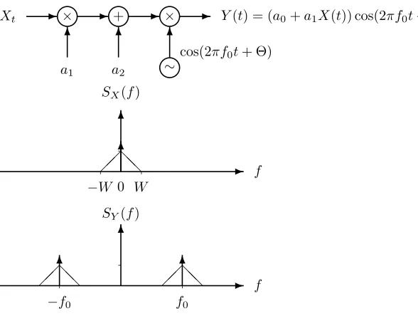
5.5 Linear Modulation . . . 298
5.6 White Noise . . . 301
5.7 Time-Averages . . . 305
5.8 Differentiating Random Processes . . . 309
5.9 Linear Estimation and Filtering . . . 312
5.10 Problems . . . 326
6 A Menagerie of Processes 343 6.1 Discrete Time Linear Models . . . 344
6.2 Sums of IID Random Variables . . . 348
6.3 Independent Stationary Increments . . . 350
6.4 Second-Order Moments of ISI Processes . . . 353
6.5 Specification of Continuous Time ISI Processes . . . 355
6.6 Moving-Average and Autoregressive Processes . . . 358
6.7 The Discrete Time Gauss-Markov Process . . . 360
6.8 Gaussian Random Processes . . . 361
6.9 The Poisson Counting Process . . . 361
6.10 Compound Processes . . . 364
6.11 Exponential Modulation . . . 366
6.12 Thermal Noise . . . 371
6.13 Ergodicity and Strong Laws of Large Numbers . . . 373
A Preliminaries 389
A.1 Set Theory . . . 389
A.2 Examples of Proofs . . . 397
A.3 Mappings and Functions . . . 401
A.4 Linear Algebra . . . 402
A.5 Linear System Fundamentals . . . 405
A.6 Problems . . . 410
B Sums and Integrals 417 B.1 Summation . . . 417
B.2 Double Sums . . . 420
B.3 Integration . . . 421
B.4 The Lebesgue Integral . . . 423
C Common Univariate Distributions 427
D Supplementary Reading 429
Bibliography 434
Preface
The origins of this book lie in our earlier bookRandom Processes: A Math-ematical Approach for Engineers, Prentice Hall, 1986. This book began as a second edition to the earlier book and the basic goal remains unchanged — to introduce the fundamental ideas and mechanics of random processes to engineers in a way that accurately reflects the underlying mathematics, but does not require an extensive mathematical background and does not belabor detailed general proofs when simple cases suffice to get the basic ideas across. In the thirteen years since the original book was published, however, numerous improvements in the presentation of the material have been suggested by colleagues, students, teaching assistants, and by our own teaching experience. The emphasis of the class shifted increasingly towards examples and a viewpoint that better reflected the course title: An Intro-duction to Statistical Signal Processing. Much of the basic content of this course and of the fundamentals of random processes can be viewed as the analysis of statistical signal processing systems: typically one is given a probabilistic description for one random object, which can be considered as aninput signal. An operation or mapping or filtering is applied to the input signal (signal processing) to produce a new random object, the out-put signal. Fundamental issues include the nature of the basic probabilistic description and the derivation of the probabilistic description of the output signal given that of the input signal and a description of the particular oper-ation performed. A perusal of the literature in statistical signal processing, communications, control, image and video processing, speech and audio processing, medical signal processing, geophysical signal processing, and classical statistical areas of time series analysis, classification and regres-sion, and pattern recognition show a wide variety of probabilistic models for input processes and for operations on those processes, where the operations might be deterministic or random, natural or artificial, linear or nonlinear, digital or analog, or beneficial or harmful. An introductory course focuses on the fundamentals underlying the analysis of such systems: the theories of probability, random processes, systems, and signal processing.
When the original book went out of print, the time seemed ripe to convert the manuscript from the prehistoric troff to LATEX and to undertake a serious revision of the book in the process. As the revision became more extensive, the title changed to match the course name and content. We reprint the original preface to provide some of the original motivation for the book, and then close this preface with a description of the goals sought during the revisions.
Preface to
Random Processes: An Introduction for
Engineers
Nothing in nature is random . . . A thing appears random only through the incompleteness of our knowledge. — Spinoza,
Ethics I
I do not believe that God rolls dice. — attributed to Einstein Laplace argued to the effect that given complete knowledge of the physics of an experiment, the outcome must always be predictable. This metaphys-ical argument must be tempered with several facts. The relevant param-eters may not be measurable with sufficient precision due to mechanical or theoretical limits. For example, the uncertainty principle prevents the simultaneous accurate knowledge of both position and momentum. The deterministic functions may be too complex to compute in finite time. The computer itself may make errors due to power failures, lightning, or the general perfidy of inanimate objects. The experiment could take place in a remote location with the parameters unknown to the observer; for ex-ample, in a communication link, the transmitted message is unknown a priori,for if it were not, there would be no need for communication. The results of the experiment could be reported by an unreliable witness — either incompetent or dishonest. For these and other reasons, it is useful to have a theory for the analysis and synthesis of processes that behave in a random or unpredictable manner. The goal is to construct mathematical models that lead to reasonably accurate prediction of the long-term average behavior of random processes. The theory should produce good estimates of the average behavior of real processes and thereby correct theoretical derivations with measurable results.
elementary discrete and continuous time linear systems theory, elementary probability, and transform theory and applications. Detailed proofs are presented only when within the scope of this background. These simple proofs, however, often provide the groundwork for “handwaving” justifi-cations of more general and complicated results that are semi-rigorous in that they can be made rigorous by the appropriate delta-epsilontics of real analysis or measure theory. A primary goal of this approach is thus to use intuitive arguments that accurately reflect the underlying mathematics and which will hold upunder scrutiny if the student continues to more advanced courses. Another goal is to enable the student who might not continue to more advanced courses to be able to read and generally follow the modern literature on applications of random processes to information and commu-nication theory, estimation and detection, control, signal processing, and stochastic systems theory.
Revision
The most recent (summer 1999) revision fixed numerous typos reported during the previous year and added quite a bit of material on jointly Gaus-sian vectors in Chapters 3 and 4 and on minimum mean squared error estimation of vectors in Chapter 4.
This revision is a work in progress. Revised versions will be made avail-able through the World Wide Web page
http://www-isl.stanford.edu/~gray/sp.html . The material is copyrighted by the authors, but is freely available to any who wish to use it provided only that the contents of the entire text remain intact and together. A copyright release form is available for printing the book at the Web page. Comments, corrections, and suggestions should be sent [email protected]. Every effort will be made to fix typos and take suggestions into an account on at least an annual basis.
Acknowledgements
We repeat our acknowledgements of the original book: to Stanford Univer-sity and the UniverUniver-sity of Maryland for the environments in which the book was written, to the John Simon Guggenheim Memorial Foundation for its support of the first author, to the Stanford University Information Systems Laboratory Industrial Affiliates Program which supported the computer facilities used to compose this book, and to the generations of students who suffered through the ever changing versions and provided a stream of comments and corrections. Thanks are also due to Richard Blahut and anonymous referees for their careful reading and commenting on the orig-inal book, and to the many who have provided corrections and helpful suggestions through the Internet since the revisions began being posted. Particular thanks are due to Yariv Ephraim for his continuing thorough and helpful editorial commentary.
Glossary
{ } a collection of points satisfying some property, e.g., {r :r≤a} is the collection of all real numbers less than or equal to a valuea
[ ] an interval of real points including the end points, e.g., for a ≤ b [a, b] ={r:a≤r≤b}. Called aclosed interval.
( ) an interval of real points excluding the end points, e.g., for a ≤ b (a, b) = {r : a < r < b}.Called an open interval. . Note this is empty if a=b.
( ], [ ) denote intervals of real points including one endpoint and exclud-ing the other, e.g., fora≤b(a, b] ={r:a < r≤b}, [a, b) ={r:a≤r < b}.
∅ The empty set, the set that contains no points.
Ω The sample space or universal set, the set that contains all of the points.
F Sigma-field or event space
P probability measure
PX distribution of a random variable or vectorX
pX probability mass function (pmf) of a random variableX
fX probability density function (pdf) of a random variableX
FX cumulative distribution function (cdf) of a random variableX
E(X) expectation of a random variableX
MX(ju) characteristic function of a random variableX
1F(x) indicator function of a setF
Φ Phi function (Eq. (2.78))
Chapter 1
Introduction
A random or stochastic process is a mathematical model for a phenomenon that evolves in time in an unpredictable manner from the viewpoint of the observer. The phenomenon may be a sequence of real-valued measurements of voltage or temperature, a binary data stream from a computer, a mod-ulated binary data stream from a modem, a sequence of coin tosses, the daily Dow-Jones average, radiometer data or photographs from deep space probes, a sequence of images from a cable television, or any of an infinite number of possible sequences, waveforms, or signals of any imaginable type. It may be unpredictable due to such effects as interference or noise in a com-munication link or storage medium, or it may be an information-bearing signal-deterministic from the viewpoint of an observer at the transmitter but random to an observer at the receiver.
The theory of random processes quantifies the above notions so that one can construct mathematical models of real phenomena that are both tractable and meaningful in the sense of yielding useful predictions of fu-ture behavior. Tractability is required in order for the engineer (or anyone else) to be able to perform analyses and syntheses of random processes, perhaps with the aid of computers. The “meaningful” requirement is that the models provide a reasonably good approximation of the actual phe-nomena. An oversimplified model may provide results and conclusions that do not apply to the real phenomenon being modeled. An overcomplicated one may constrain potential applications, render theory too difficult to be useful, and strain available computational resources. Perhaps the most dis-tinguishing characteristic between an average engineer and an outstanding engineer is the ability to derive effective models providing a good balance between complexity and accuracy.
ronments or systems whichchangethe processes to produce other processes. The intentional operation on a signal produced by one process, an “input signal,” to produce a new signal, an “output signal,” is generally referred to assignal processing, a topic easily illustrated by examples.
• A time varying voltage waveform is produced by a human speaking into a microphone or telephone. This signal can be modeled by a random process. This signal might be modulated for transmission, it might be digitized and coded for transmission on a digital link, noise in the digital link can cause errors in reconstructed bits, the bits can then be used to reconstruct the original signal within some fidelity. All of these operations on signals can be considered as signal processing, although the name is most commonly used for the man-made operations such as modulation, digitization, and coding, rather than the natural possibly unavoidable changes such as the addition of thermal noise or other changes out of our control.
• For very low bit rate digital speech communication applications, the speech is sometimes converted into a model consisting of a simple linear filter (called an autoregressive filter) and an input process. The idea is that the parameters describing the model can be communicated with fewer bits than can the original signal, but the receiver can synthesize the human voice at the other end using the model so that it sounds very much like the original signal.
• Signals including image data transmitted from remote spacecraft are virtually buried in noise added to them on route and in the front end amplifiers of the powerful receivers used to retrieve the signals. By suitably preparing the signals prior to transmission, by suitable filtering of the received signal plus noise, and by suitable decision or estimation rules, high quality images have been transmitted through this very poor channel.
• Signals produced by biomedical measuring devices can display spe-cific behavior when a patient suddenly changes for the worse. Signal processing systems can look for these changes and warn medical per-sonnel when suspicious behavior occurs.
Courses and texts on random processes usually fall into either of two general and distinct categories. One category is the common engineering approach, which involves fairly elementary probability theory, standard un-dergraduate Riemann calculus, and a large dose of “cookbook” formulas — often with insufficient attention paid to conditions under which the formu-las are valid. The results are often justified by nonrigorous and occasionally mathematically inaccurate handwaving or intuitive plausibility arguments that may not reflect the actual underlying mathematical structure and may not be supportable by a precise proof. While intuitive arguments can be extremely valuable in providing insight into deep theoretical results, they can be a handicap if they do not capture the essence of a rigorous proof.
A development of random processes that is insufficiently mathematical leaves the student ill prepared to generalize the techniques and results when faced with a real-world example not covered in the text. For example, if one is faced with the problem of designing signal processing equipment for predicting or communicating measurements being made for the first time by a space probe, how does one construct a mathematical model for the physical process that will be useful for analysis? If one encounters a process that is neither stationary nor ergodic, what techniques still apply? Can the law of large numbers still be used to construct a useful model?
An additional problem with an insufficiently mathematical development is that it does not leave the student adequately prepared to read modern literature such as the manyTransactions of the IEEE. The more advanced mathematical language of recent work is increasingly used even in simple cases because it is precise and universal and focuses on the structure com-mon to all random processes. Even if an engineer is not directly involved in research, knowledge of the current literature can often provide useful ideas and techniques for tackling specific problems. Engineers unfamiliar with basic concepts such assigma-fieldandconditional expectationwill find many potentially valuable references shrouded in mystery.
This book attempts a compromise between the two approaches by giving the basic, elementary theory and a profusion of examples in the language and notation of the more advanced mathematical approaches. The intent is to make the crucial concepts clear in the traditional elementary cases, such as coin flipping, and thereby to emphasize the mathematical structure of all random processes in the simplest possible context. The structure is then further developed by numerous increasingly complex examples of ran-dom processes that have proved useful in stochastic systems analysis. The complicated examples are constructed from the simple examples by signal processing, that is, by using a simple process as an input to a system whose output is the more complicated process. This has the double advantage of describing the action of the system, the actual signal processing, and the interesting random process which is thereby produced. As one might suspect, signal processing can be used to produce simple processes from complicated ones.
Careful proofs are constructed only in elementary cases. For example, the fundamental theorem of expectation is proved only for discrete random variables, where it is proved simply by a change of variables in a sum. The continuous analog is subsequently given without a careful proof, but with the explanation that it is simply the integral analog of the summation formula and hence can be viewed as a limiting form of the discrete result. As another example, only weak laws of large numbers are proved in detail in the mainstream of the text, but the stronger laws are at least stated and they are discussed in some detail in starred sections.
By these means we strive to capture the spirit of important proofs with-out undue tedium and to make plausible the required assumptions and con-straints. This, in turn, should aid the student in determining when certain tools do or do not apply and what additional tools might be necessary when new generalizations are required.
permits a more complete discussion of processes that violate such proba-bilistic regularity requirements yet still have useful relations between time and probabilistic averages.
Even though a student completing this book will not be able to fol-low the details in the literature of many proofs of results involving random processes, the basic results and their development and implications should be accessible, and the most common examples of random processes and classes of random processes should be familiar. In particular, the student should be well equipped to follow the gist of most arguments in the vari-ousTransactions of the IEEEdealing with random processes, including the
IEEE Transactions on Signal Processing,IEEE Transactions on Image Pro-cessing,IEEE Transactions on Speech and Audio Processing,IEEE Trans-actions on Communications, IEEE Transactions on Control, and IEEE Transactions on Information Theory.
It also should be mentioned that the authors are electrical engineers and, as such, have written this text with an electrical engineering flavor. However, the required knowledge of classical electrical engineering is slight, and engineers in other fields should be able to follow the material presented. This book is intended to provide a one-quarter or one-semester course that develops the basic ideas and language of the theory of random pro-cesses and provides a rich collection of examples of commonly encountered processes, properties, and calculations. Although in some cases these ex-amples may seem somewhat artificial, they are chosen to illustrate the way engineers should think about random processes and for simplicity and con-ceptual content rather than to present the method of solution to some particular application. Sections that can be skimmed or omitted for the shorter one-quarter curriculum are marked with a star (). Discrete time processes are given more emphasis than in many texts because they are simpler to handle and because they are of increasing practical importance in and digital systems. For example, linear filter input/output relations are carefully developed for discrete time and then the continuous time analogs are obtained by replacing sums with integrals.
Most examples are developed by beginning with simple processes and then filtering or modulating them to obtain more complicated processes. This provides many examples of typical probabilistic computations and output of operations on simple processes. Extra tools are introduced as needed to develop properties of the examples.
material can by found, for example, in Gray and Goodman [23]. Although some of these basic topics are reviewed in this book in appendix A, they are considered prerequisite as the pace and density of material would likely be overwhelming to someone not already familiar with the fundamental ideas of probability such as probability mass and density functions (including the more common named distributions), computing probabilities, derived dis-tributions, random variables, and expectation. It has long been the authors’ experience that the students having the most difficulty with this material are those with little or no experience with elementary probability.
Organization of the Book
Chapter 2 provides a careful development of the fundamental concept of probability theory — a probability space or experiment. The notions of sample space, event space, and probability measure are introduced, and several examples are toured. Independence and elementary conditional probability are developed in some detail. The ideas of signal processing and of random variables are introduced briefly as functions or operations on the output of an experiment. This in turn allows mention of the idea of expectation at an early stage as a generalization of the description of probabilities by sums or integrals.
Chapter 3 treats the theory of measurements made on experiments: random variables, which are scalar-valued measurements; random vectors, which are a vector or finite collection of measurements; and random pro-cesses, which can be viewed as sequences or waveforms of measurements. Random variables, vectors, and processes can all be viewed as forms of sig-nal processing: each operates on “inputs,” which are the sample points of a probability space, and produces an “output,” which is the resulting sam-ple value of the random variable, vector, or process. These output points together constitute an output sample space, which inherits its own proba-bility measure from the structure of the measurement and the underlying experiment. As a result, many of the basic properties of random variables, vectors, and processes follow from those of probability spaces. Probability distributions are introduced along with probability mass functions, proba-bility density functions, and cumulative distribution functions. The basic derived distribution method is described and demonstrated by example. A wide variety of examples of random variables, vectors, and processes are treated.
can be thought of as providing simple but important parameters describ-ing probability distributions. A variety of specific averages are considered, including mean, variance, characteristic functions, correlation, and covari-ance. Several examples of unconditional and conditional expectations and their properties and applications are provided. Perhaps the most impor-tant application is to the statement and proof of laws of large numbers or ergodic theorems, which relate long term sample average behavior of ran-dom processes to expectations. In this chapter laws of large numbers are proved for simple, but important, classes of random processes. Other im-portant applications of expectation arise in performing and analyzing signal processing applications such as detecting, classifying, and estimating data. Minimum mean squared nonlinear and linear estimation of scalars and vec-tors is treated in some detail, showing the fundamental connections among conditional expectation, optimal estimation, and second order moments of random variables and vectors.
Chapter 5 concentrates on the computation of second-order moments — the mean and covariance — of a variety of random processes. The primary example is a form of derived distribution problem: if a given random process with known second-order moments is put into a linear system what are the second-order moments of the resulting output random process? This prob-lem is treated for linear systems represented by convolutions and for linear modulation systems. Transform techniques are shown to provide a simpli-fication in the computations, much like their ordinary role in elementary linear systems theory. The chapter closes with a development of several results from the theory of linear least-squares estimation. This provides an example of both the computation and the application of second-order moments.
independent increment processes, Markov processes, Poisson and Gaussian processes, and the random telegraph wave. We also briefly consider an ex-ample of a nonlinear system where the output random processes can at least be partially described — the exponential function of a Gaussian or Poisson process which models phase or frequency modulation. We close with ex-amples of a type of “doubly stochastic” process, compound processes made upby adding a random number of other random effects.
Appendix A sketches several prerequisite definitions and concepts from elementary set theory and linear systems theory using examples to be en-countered later in the book. The first subject is crucial at an early stage and should be reviewed before proceeding to chapter 2. The second subject is not required until chapter 5, but it serves as a reminder of material with which the student should already be familiar. Elementary probability is not reviewed, as our basic development includes elementary probability. The review of prerequisite material in the appendix serves to collect together some notation and many definitions that will be used throughout the book. It is, however, only a brief review and cannot serve as a substitute for a complete course on the material. This chapter can be given as a first reading assignment and either skipped or skimmed briefly in class; lectures can proceed from an introduction, perhaps incorporating some preliminary material, directly to chapter 2.
Appendix B provides some scattered definitions and results needed in the book that detract from the main development, but may be of interest for background or detail. These fall primarily in the realm of calculus and range from the evaluation of common sums and integrals to a consideration of different definitions of integration. Many of the sums and integrals should be prerequisite material, but it has been the authors’ experience that many students have either forgotten or not seen many of the standard tricks and hence several of the most important techniques for probability and signal processing applications are included. Also in this appendix some background information on limits of double sums and the Lebesgue integral is provided.
Appendix C collects the common univariate pmf’s and pdf’s along with their second order moments for reference.
further study, not as an exhaustive description of the relevant literature, the latter goal being beyond the authors’ interests and stamina.
Chapter 2
Probability
2.1
Introduction
The theory of random processes is a branch of probability theory and prob-ability theory is a special case of the branch of mathematics known as measure theory. Probability theory and measure theory both concentrate on functions that assign real numbers to certain sets in an abstract space according to certain rules. These set functions can be viewed as measures of the size or weight of the sets. For example, the precise notion of area in two-dimensional Euclidean space and volume in three-dimensional space are both examples of measures on sets. Other measures on sets in three dimensions are mass and weight. Observe that from elementary calculus we can find volume by integrating a constant over the set. From physics we can find mass by integrating a mass density or summing point masses over a set. In both cases the set is a region of three-dimensional space. In a similar manner, probabilities will be computed by integrals of densities of probability or sums of “point masses” of probability.
Both probability theory and measure theory consider only nonnegative real-valued set functions. The value assigned by the function to a set is called the probability or the measure of the set, respectively. The basic difference between probability theory and measure theory is that the former considers only set functions that are normalized in the sense of assigning the value of 1 to the entire abstract space, corresponding to the intuition that the abstract space contains every possible outcome of an experiment and hence should happen with certainty or probability 1. Subsets of the space have some uncertainty and hence have probability less than 1.
Probability theory begins with the concept of aprobability space, which is a collection of three items:
1. An abstract space Ω, such as encountered in appendix A, called a
sample space, which contains all distinguishableelementary outcomes
or results of an experiment. These points might be names, numbers, or complicated signals.
2. Anevent space or sigma-field F consisting of a collection of subsets of the abstract space which we wish to consider as possible events and to which we wish to assign a probability. We require that the event space have an algebraic structure in the following sense: any finite or infinite sequence of set-theoretic operations (union, intersection, complementation, difference, symmetric difference) on events must produce other events, even countably infinite sequences of operations. 3. Aprobability measureP — an assignment of a number between 0 and 1 to every event, that is, to every set in the event space. A probability measure must obey certain rules oraxioms and will be computed by integrating or summing, analogous to area, volume, and mass. This chapter is devoted to developing the ideas underlying the triple (Ω,F, P), which is collectively called aprobability spaceor an experiment. Before making these ideas precise, however, several comments are in order. First of all, it should be emphasized that a probability space is composed of three parts; an abstract space is only one part. Do not let the terminology confuse you: “space” has more than one usage. Having an abstract space model all possible distinguishable outcomes of an experiment should be an intuitive idea since it is simply giving a precise mathematical name to an imprecise English description. Since subsets of the abstract space correspond to collections of elementary outcomes, it should also be possible to assign probabilities to such sets. It is a little harder to see, but we can also argue that we should focus on the sets and not on the individual points when assigning probabilities since in many cases a probability assignment known only for points will not be very useful. For example, if we spin a fair pointer and the outcome is known to be equally likely to be any number between 0 an 1, then the probability that any particular point such as .3781984637 or exactly 1/π occurs is 0 because there are an uncountable infinity of possible points, none more likely than the others1. Hence knowing only that the probability of each and every point is zero, we would be hard
1A set is countably infinite if it can be put into one-to-one correspondence
pressed to make any meaningful inferences about the probabilities of other events such as the outcome being between 1/2 and 3/4. Writers of fiction (including Patrick O’Brian in his Aubrey-Maturin series) have often made much of the fact that extremely unlikely events often occur. One can say that zero probability events occur all virtually all the time since thea priori
probability that the universe will be exactly a particular configuration at 12:01AM Coordinated Universal Time (aka Greenwich Mean Time) is 0, yet the universe will indeed be in some configuration at that time.
The difficulty inherent in this example leads to a less natural aspect of the probability space triumvirate — the fact that we must specify an event space or collection of subsets of our abstract space to which we wish to assign probabilities. In the example it is clear that taking the individual points and their countable combinations is not enough (see also problem 2.2). On the other hand, why not just make the event space the class of
all subsets of the abstract space? Why require the specification of which subsets are to be deemed sufficiently important to be blessed with the name “event”? In fact, this concern is one of the principal differences between elementary probability theory and advanced probability theory (and the point at which the student’s intuition frequently runs into trouble). When the abstract space is finite or even countably infinite, one can consider all possible subsets of the space to be events, and one can build a useful theory. When the abstract space is uncountably infinite, however, as in the case of the space consisting of the real line or the unit interval, one cannot build a useful theory without constraining the subsets to which one will assign a probability. Roughly speaking, this is because probabilities of sets in uncountable spaces are found by integrating over sets, and some sets are simply too nasty to be integrated over. Although it is difficult to show, for such spaces there does not exist a reasonable and consistent means of assigning probabilities to all subsets without contradiction or without violating desirable properties. In fact, is is so difficult to show that such “non-probability-measurable” subsets of the real line exist that we will not attempt to do so in this book. The reader should at least be aware of the problem so that the need for specifying an event space is understood. It also explains why the reader is likely to encounter phrases like “measurable sets” and “measurable functions” in the literature.
intersections of events (corresponding to a logical “and”), then the resulting sets are also events and hence will have probabilities. In fact, this is one of the main functions of probability theory: given a probabilistic description of a collection of events, find the probability of some new event formed by set-theoretic operations on the given events.
Upto this point the notion ofsignal processinghas not been mentioned. It enters at a fundamental level if one realizes that each individual point ω∈Ω produced in an experiment can be viewed as asignal, it might be a single voltage conveying the value of a measurement, a vector of values, a sequence of values, or a waveform, any one of which can be interpreted as a
signal measured in the environment or received from a remote transmitter or extracted from a physical medium that was previously recorded. Signal processing in general is the performing of some operation on the signal. In its simplest yet most general form this consists of applying some function or mapping or operationgto the signal or inputωto produce an outputg(ω), which might be intended to guess some hidden parameter, extract useful information from noise, enhance an image, or any simple or complicated operation intended to produce a useful outcome. If we have a probabilistic description of the underlying experiment, then we should be able to derive a probabilistic description of the outcome of the signal processor. This, in fact, is the core problem of derived distributions, one of the fundamental tools of both probability theory and signal processing. In fact, this idea of defining functions on probability spaces is the foundation for the definition of random variables, random vectors, and random processes, which will in-herit their basic properties from the underlying probability space, thereby yielding new probability spaces. Much of the theory of random processes and signal processing consists of developing the implications of certain oper-ations on probability spaces: beginning with some probability space we form new ones by operations called variously mappings, filtering, sampling, cod-ing, communicatcod-ing, estimatcod-ing, detectcod-ing, averagcod-ing, measurcod-ing, enhanc-ing, predictenhanc-ing, smoothenhanc-ing, interpolatenhanc-ing, classifyenhanc-ing, analyzing or other names denoting linear or nonlinear operations. Stochastic systems theory is the combination of systems theory with probability theory. The essence of stochastic systems theory is the connection of a system to a probability space. Thus a precise formulation and a good understanding of probability spaces are prerequisites to a precise formulation and correct development of examples of random processes and stochastic systems.
2.2
Spinning Pointers and Flipping Coins
Many of the basic ideas at the core of this text can be introduced and illus-trated by two very simple examples, the continuous experiment of spinning a pointer inside a circle and the discrete experiment of flipping a coin.
A Uniform Spinning Pointer
Suppose that Nature (or perhaps Tyche, the Greek Goddess of chance) spins a pointer in a circle as depicted in Figure 2.1. When the pointer stops it can
✫✪ ✬✩
✻
0.0
0.5 0.25 0.75
Figure 2.1: The Spinning Pointer
in the interval [a, b]” is
P([a, b]) =b−a. (2.1)
We do not have to restrict interest to intervals in order to define probabil-ities consistent with (2.1). The notion of the length of an interval can be made precise using calculus and simultaneously extended to any subset of [0,1) by defining the probabilityP(F) of a setF⊂[0,1) as
P(F)∆=
F
f(r)dr=
1F(r)f(r)dr, (2.2)
wheref(r) = 1 for allr∈[0,1). With this definition it is clear that for any 0≤a < b≤1 that
P([a, b]) =
b
a
f(r)dr=b−a. (2.3)
We could also arrive at effectively the same model by considering the sample space to be the entire real line, Ω == (−∞,∆ ∞) and defining the pdf to be
f(r) =
1 ifr∈[0,1)
0 otherwise . (2.4)
The integral can also be expressed without specifying limits of integration by using the indicator function of a set
1F(r) =
1 ifr∈F
0 ifr∈F (2.5)
as
P(F)=∆
1F(r)f(r)dr. (2.6)
computing the probability of an interval, then both formulas must give the same numerical result — as they do in this example.
The second implicit assumption is that the integral exists in a well de-fined sense, that it can be evaluated using calculus. As surprising as it may seem to readers familiar only with typical engineering-oriented devel-opments of Riemann integration, the integral of (2.2) is in fact not well defined for all subsets of [0,1). But we leave this detail for later and as-sume for the moment that we only encounter sets for which the integral (and hence the probability) is well defined.
The functionf(r) is called aprobability density functionorpdf since it is a nonnegative point function that is integrated to compute total probability of a set, just as a mass density function is integrated over a region to compute the mass of a region in physics. Since in this example f(r) is constant over a region, it is called auniform pdf..
The formula (2.2) for computing probability has many implications, three of which merit comment at this point.
•Probabilities are nonnegative:
P(F)≥0 for anyF. (2.7)
This follows since integrating a nonnegative argument yields a nonnegative result.
•The probability of the entire sample space is 1:
P(Ω) = 1. (2.8)
This follows since integrating 1 over the unit interval yields 1, but it has the intuitive interpretation that the probability that “something happens” is 1.
• The probability of the union of disjoint regions is the sum of the proba-bilities of the individual events:
IfF∩G=∅, thenP(F∪G) =P(F) +P(G). (2.9) This follows immediately from the properties of integration:
P(F∪G) =
F∪G
f(r)dr
=
F
f(r)dr+
G
f(r)dr = P(F) +P(G).
1F∪G(r) = 1F(r) + 1G(r) and hence linearity of integration implies that
P(F∪G) =
1F∪G(r)f(r)dr
=
(1F(r) + 1G(r))f(r)dr
=
1F(r)f(r)dr+
1G(r)f(r)dr
= P(F) +P(G).
This property is often called the additivity property of probability. The second proof makes it clear that additivity of probability is an immediate result of the linearity of integration, i.e., that the integral of the sum of two functions is the sum of the two integrals.
Repeated application of additivity for two events shows that for any finite collection {Fk; k = 1,2, . . . , K} of disjoint or mutually exclusive
events, i.e., events with the property that Fk
Fj =∅ for all k =j, we
have that
P(
K
k=1 Fk) =
K
k=1
P(Fk), (2.10)
showing that additivity is equivalent to finite additivity, the similar prop-erty for finite sets instead of just two sets. Since additivity is a special case of finite additivity, the two notions are equivalent and we can use them interchangably.
These three properties of nonnegativity, normalization, and additivity are fundamental to the definition of the general notion of probability and will form three of the four axioms needed for a precise development. It is tempting to call an assignment P of numbers to subsets of a sample space a probability measure if it satisfies these three properties, but we shall see that a fourth condition, which is crucial for having well behaved limits and asymptotics, will be needed to complete the definition. Pending this fourth condition, (2.2) defines a probability measure. A sample space together with a probability measure provide a mathematical model for an experiment. This model is often called a probability space, but for the moment we shall stick to the less intimidating word ofexperiment.
Simple Properties
Assume thatPis a set function defined on a sample space Ω that satisfies properties (2.7 – 2.9). Then
(a) P(Fc) = 1−P(F).
(b) P(F)≤1 .
(c) Let∅ be the null or empty set, thenP(∅) = 0.
(d) If {Fi; i = 1,2, . . . , K} is a finite partition of Ω, i.e., if Fi∩Fk = ∅
wheni=k andi=1Fi = Ω, then
P(G) =
K
i=1
P(G∩Fi) (2.11)
for any eventG.
Proof:
(a) F∪Fc= Ω impliesP(F∪Fc) = 1 (property 2.8). F∩Fc=∅implies
1 =P(F∪Fc) =P(F) +P(Fc) (property 2.9), which implies (a).
(b) P(F) = 1−P(Fc)≤1 (property 2.7 and (a) above).
(c) By property 2.8 and (a) above, P(Ωc) =P(∅) = 1−P(Ω) = 0.
(d) P(G) =P(G∩Ω) =P(G∩(
i
Fi)) =P(
i
(G∩Fi)) =
i
P(G∩Fi).
Observe that although the null or empty set ∅ has probability 0, the converse is not true in that a set need not be empty just because it has zero probability. In the uniform fair wheel example the setF ={1/n:n= 1,2,3, . . .} is not empty, but it does have probability zero. This follows rougly because for any finite N P({1/n : n = 1,2,3, . . . , N}) = 0 and therefore the limit asN→ ∞must also be zero.
A Single Coin Flip
Ω ={0,1} and the probability for any event or subset ofω can be defined in a reasonable way by
P(F) =
r∈F
p(r), (2.12)
or, equivalently,
P(F) =1F(r)p(r), (2.13)
where now p(r) = 1/2 for each r ∈ Ω. The function p is called a proba-bility mass function orpmf because it is summed over points to find total probability, just as point masses are summed to find total mass in physics. Be cautioned thatP is defined for sets andpis defined only for points in the sample space. This can be confusing when dealing with one-point or singleton sets, for example
P({0}) = p(0) P({1}) = p(1).
This may seem too much work for such a little example, but keep in mind that the goal is a formulation that will work for far more complicated and interesting examples. This example is different from the spinning wheel in that the sample space is discrete instead of continuous and that the probabilities of events are defined by sums instead of integrals, as one should expect when doing discrete math. It is easy to verify, however, that the basic properties (2.7)–(2.9) hold in this case as well (since sums behave like integrals), which in turn implies that the simple properties (a)–(b) also hold.
A Single Coin Flip as Signal Processing
The coin flip example can also be derived in a very different way that pro-vides our first example of signal processing. Consider again the spinning pointer so that the sample space is Ω and the probability measureP is de-scribed by (2.2) using a uniform pdf as in (2.4). Performing the experiment by spinning the pointer will yield some real number r ∈ [0,1). Define a measurementqmade on this outcome by
q(r) =
1 ifr∈[0,0.5]
This function can also be defined somewhat more economically as
q(r) = 1[0,0.5](r). (2.15)
This is an example of a quantizer, an operation that maps a continuous value into a discrete one. Quantization is an example ofsignal processing
since it is a function or mapping defined on an input space, here Ω = [0,1) or Ω = , producing a value in some output space, here a binary space Ωg = {0,1}. The dependence of a function on its input space or domain
of definition Ω and its output space or range Ωg,is often denoted by q :
Ω→Ωg. Although introduced as an example of simple signal processing,
the usual name for a real-valued function defined on the sample space of a probability space is arandom variable. We shall see in the next chapter that there is an extra technical condition on functions to merit this name, but that is a detail that can be postponed.
The output space Ωgcan be considered as a new sample space, the space
corresponding to the possible values seen by an observer of the output of the quantizer (an observer who might not have access to the original space). If we know both the probability measure on the input space and the function, then in theory we should be able to describe the probability measure that the output space inherits from the input space. Since the output space is discrete, it should be described by a pmf, saypq. Since there are only two
points, we need only find the value ofpq(1) (orpq(0) sincepq(0)+pq(1) = 1).
On output of 1 is seen if and only if the input sample point lies in [0,0.5], so it follows easily thatpq(0) =P([0,0.5]) =
0.5
0 f(r), dr= 0.5, exactly the value assumed for the fair coin flipmodel. The pmfpq implies a probability
measure on the output space Ωg by
Pq(F) =
ω∈F
pq(ω),
where the subscriptqdistinguishes the probability measurePq on the
out-put space from the probability measure P on the input space. Note that we can define any other binary quantizer corresponding to an “unfair” or biased coin by changing the 0.5 to some other value.
This simple example makes several fundamental points that will evolve in depth in the course of this material. First, it provides an example of
of a common phenomenon that quite different models can result in iden-tical sample spaces and probability measures. Here the coin flip could be modeled in a directly given fashion by just describing the sample space and the probability measure, or it can be modeled in an indirect fashion as a function (signal processing, random variable) on another experiment. This suggests, for example, that to study coin flips empirically we could either actually flipa fair coin, or we could spin a fair wheel and quantize the output. Although the second method seems more complicated, it is in fact extremely common since most random number generators (or pseudo-random number generators) strive to produce pseudo-random numbers with a uni-form distribution on [0,1) and all other probability measures are produced by further signal processing. We have seen how to do this for a simple coin flip. In fact any pdf or pmf can be generated in this way. (See problem 3.7.) The generation of uniform random numbers is both a science and an art. Most function roughly as follows. One begins with floating point number in (0,1) called theseed, saya, and uses another postive floating point num-ber, sayb, as a multiplier. A sequence xn is then generated recursively as
x0=aandxn=b×xn−1 mod (1) forn= 1,2, . . ., that is, the fractional
part of b×xn−1. If the two numbers a and b are suitably chosen then
xn should appear to be uniform. (Try it!) In fact, since there are only
a finite number (albeit large) of possible numbers that can be represented on a digital computer, this algorithm must eventually repeat and hencexn
must be a periodic sequence. The goal of designing a good pseudo-random number generater is to make the period as long as possible and to make the sequences produced look as much as possible like a random sequence in the sense that statistical tests for independence are fooled.
Abstract vs. Concrete
It may seem strange that the axioms of probability deal with apparently abstract ideas of measures instead of corresponding physical intuition that the probability tells you something about the fraction of times specific events will occur in a sequence of trials, such as the relative frequency of a pair of dice summing to seven in a sequence of many roles, or a decision algorithm correctly detecting a single binary symbol in the presence of noise in a transmitted data file. Such real world behavior can be quantified by the idea of a relative frequency, that is, suppose the output of thenth of a sequence of trials isxn and we wish to know the relative frequency thatxn
takes on a particular value, saya. Then given an infinite sequence of trials x={x0, x1, x2, . . .}we could define the relative frequency ofainxby
ra(x) = lim n→∞
number ofk∈ {0,1, . . . , n−1}for whichxk=a
For example, the relative frequency of heads in an infinite sequence of fair coin flips should be 0.5, the relative frequency of rolling a pair of fair dice and having the sum be 7 in an infinite sequence of rolls should be 1/6 since the pairs (1,6),(6,1),(2,5),(5,2),(3,4),(4,3) are equally likely and form 6 of the possible 36 pairs of outcomes. Thus one might suspect that to make a rigorous theory of probability requires only a rigorous definition of probabilities as such limits and a reaping of the resulting benefits. In fact much of the history of theoretical probability consisted of attempts to accomplish this, but unfortunately it does not work. Such limits might not exist, or they might exist and not converge to the same thing for different repetitions of the same experiment. Even when the limits do exist there is no guarantee they will behave as intuition would suggest when one tries to do calculus with probabilities, to compute probabilities of complicated events from those of simple related events. Attempts to get around these problems uniformly failed and probability was not put on a rigorous basis until the axiomatic approach was completed by Kolmogorov. The axioms do, however, capture certain intuitive aspects of relative frequencies. Rel-ative frequencies are nonnegRel-ative, the relRel-ative frequency of the entire set of possible outcomes is one, and relative frequencies are additive in the sense that the relative frequency of the symbolaor the symbolboccurring, ra∪b(x), is clearlyra(x) +rb(x). Kolmogorov realized that beginning with
simple axioms could lead to rigorous limiting results of the type needed, while there was no way to begin with the limiting results as part of the axioms. In fact it is the fourth axiom, a limiting version of additivity, that plays the key role in making the asymptotics work.
2.3
Probability Spaces
We now turn to a more thorough development of the ideas introduced in the previous section.
Asample space Ω is an abstract space, a nonempty collection of points or members or elements calledsample points (orelementary events or ele-mentary outcomes).
An event space (or sigma-field or sigma-algebra) F of a sample space Ω is a nonempty collection of subsets of Ω calledevents with the following properties:
If F∈ F ,then also Fc∈ F , (2.17)
(review the quantizer example).
If for some finite n, Fi∈ F , i= 1,2, . . . , n, then also
n
i=1
Fi∈ F , (2.18)
that is, a finite union of events must also be an event. If Fi∈ F , i= 1,2, . . . , then also
∞
i=1
Fi∈ F , (2.19)
that is, a countable union of events must also be an event.
We shall later see alternative ways of describing (2.19), but this form is the most common.
Eq. (2.18) can be considered as a special case of (2.19) since, for exam-ple, given a finite collection Fi; i= 1, . . . , N, we can construct an infinite
sequence of sets with the same union, e.g., givenFk, k= 1,2, . . . , N,
con-struct an infinite sequence Gn with the same union by choosingGn =Fn
forn= 1,2, . . . N andGn =∅otherwise. It is convenient, however, to
con-sider the finite case separately. If a collection of sets satisfies only (2.17) and (2.18) but not 2.19, then it is called afield or algebra of sets. For this reason, in elementary probability theory one often refers to “set algebra” or to the “algebra of events.” (Don’t worry about why 2.19 might not be satisfied.) Both (2.17) and (2.18) can be considered as “closure” properties; that is, an event space must be closed under complementation and unions in the sense that performing a sequence of complementations or unions of events must yield a set that is also in the collection, i.e., a set that is also an event. Observe also that (2.17), (2.18), and (A.11) imply that
Ω∈ F , (2.20)
that is, the whole sample space considered as a set must be inF; that is, it must be an event. Intuitively, Ω is the “certain event,” the event that “something happens.” Similarly, (2.20) and (2.17) imply that
∅ ∈ F, (2.21)
A few words about the different nature of membershipin Ω andF is in order. If the setF is a subset of Ω,then we writeF ⊂Ω. If the subsetF is also in the event space, then we writeF ∈ F. Thus we use set inclusion when consideringF as a subset of an abstract space, and element inclusion when consideringF as a member of the event space and hence as an event. Alternatively, the elements of Ω are points, and a collection of these points is a subset of Ω; but the elements ofF are sets — subsets of Ω, — and not points. A student should ponder the different natures of abstract spaces of points and event spaces consisting of sets until the reasons for set inclusion in the former and element inclusion in the latter space are clear. Consider especially the difference between an element of Ω and a subset of Ω that consists of a single point. The lattermight ormight notbe an element ofF, the former isnever an element ofF.Although the difference might seem to be merely semantics, the difference is important and should be thoroughly understood.
A measurable space (Ω,F) is a pair consisting of a sample space Ω and an event space or sigma-field F of subsets of Ω. The strange name “measurable space” reflects the fact that we can assign a measure such as a probability measure, to such a space and thereby form a probability space or probability measure space.
Aprobability measure P on a measurable space (Ω,F) is an assignment of a real number P(F) to every memberF of the sigma-field (that is, to every event) such thatP obeys the following rules, which we refer to as the
axioms of probability.
Axiom 2.1
P(F)≥0 for all F ∈ F (2.22)
i.e., no event has negative probability.
Axiom 2.2
P(Ω) = 1 (2.23)
i.e., the probability of “everything” is one.
Axiom 2.3 If Fi, i= 1,2, . . . , nare disjoint, then
P
n
i=1 Fi
=
n
i=1
Axiom 2.4 If Fi, i= 1,2, . . . are disjoint, then
P
∞
i=1 Fi
=
∞
i=1
P(Fi). (2.25)
Note that nothing has been said to the effect that probabilities must be sums or integrals, but the first three axioms should be recognizable from the three basic properties of nonnegativity, normalization, and additivity encountered in the simple examples introduced in the introduction to this chapter where probabilities were defined by an integral over a set of a pdf or a sum over a set of a pmf. The axioms capture these properties in a gen-eral form and will be seen to include more gengen-eral constructions, including multidimensional integrals and combinations of integrals and sums. The fourth axiom can be viewed as an extra technical condition that must be included in order to get various limits to behave. Just as property (2.19) of an event space will later be seen to have an alternative statement in terms of limits of sets, the fourth axiom of probability, axiom 2.4, will be shown to have an alternative form in terms of explicit limits, a form providing an important continuity property of probability. Also as in the event space properties, the fourth axiom implies the third.
As with the defining properties of an event space, for the purposes of dis-cussion we have listed separately the finite special case (2.24) of the general condition (2.25). The finite special case is all that is required for elemen-tary discrete probability. The general condition is required to get a useful theory for continuous probability. A good way to think of these conditions is that they essentially describe probability measures as set functions de-fined by either summing or integrating over sets, or by some combination thereof. Hence much of probability theory is simply calculus, especially the evaluation of sums and integrals.
To emphasize an important point: a functionP which assigns numbers to elements of an event space of a sample space is a probability measureif and only if it satisfies all of the four axioms!
A probability space or experiment is a triple (Ω,F, P) consisting of a sample space Ω, an event spaceFof subsets of Ω, and a probability measure P defined for all members ofF.
space, a slight generalization of the fair coin flip permitting an unfair coin.
[2.0] Let Ω be any abstract space and letF ={Ω,∅}; that is,F consists of exactly two sets — the sample space (everything) and the empty set (nothing). This is called the trivial event space. This is a model of an experiment where only two events are possible: “Something happens” or “nothing happens” — not a very interesting description. There is only one possible probability measure for this measurable space: P(Ω) = 1 and P(∅) = 0. (Why?) This probability measure meets the required rules that define a probability measure; they can be directly verified since there are only two possible events. Equations (2.22) and (2.23) are obvious. Equations (2.24) and (2.25) follow since the only possible values for Fi are Ω and∅. At most one of theFi is
indeed Ω,then both sides of the equality are 1. Otherwise, both sides are 0.
[2.1] Let Ω = {0,1}. Let F = {{0},{1},Ω = {0,1},∅}. Since F con-tainsall of the subsets of Ω, the properties (2.17) through (2.19) are trivially satisfied, and hence it is an event space. (There is one other possible event space that could be defined for Ω in this example. What is it?) Define the set function P by
P(F) =
1−p if F ={0}
p if F ={1}
0 if F =∅
1 if F = Ω,
where p ∈(0,1) is a fixed parameter. (If p = 0 or p= 1 the space becomes trivial.) It is easily verified that P satisfies the axioms of probability and hence is a probability measure. Therefore (Ω,F, P) is a probability space. Note that we had to give the value of P(F) forall eventsF, a construction that would clearly be absurd for large sample spaces. Note also that the choice of P(F) is not unique for the given measurable space (Ω,F); we could have chosen any value in [0,1] forP({1}) and used the axioms to complete the definition. The preceding example is the simplest nontrivial example of a probabil-ity space and provides a rigorous mathematical model for applications such as the binary transmission of a single bit or for the flipping of a single bi-ased coin once. It therefore provides a complete and rigorous mathematical model for the single coin flipof the introduction.
2.3.1
Sample Spaces
Intuitively, a sample space is a listing of all conceivable finest-grain, distin-guishable outcomes of an experiment to be modeled by a probability space. Mathematically it is just an abstract space.
Examples
[2.2] A finite space Ω ={ak;k= 1,2, . . . , K}.Specific examples are the
bi-nary space{0,1}and the finite space of integersZk
∆
={0,1,2, . . . , k− 1}.
[2.3] A countably infinite space Ω = {ak;k = 0,1,2, . . .}, for some
se-quence {ak}. Specific examples are the space of all nonnegative
inte-gers{0,1,2, . . .},which we denote byZ+, and the space of all integers {. . . ,−2,−1,0,1,2, . . .},which we denote byZ. Other examples are the space of all rational numbers, the space of all even integers, and the space of all periodic sequences of integers.
Both examples [2.2] and [2.3] are called discrete spaces. Spaces with finite or countably infinite numbers of elements are called discrete spaces.
[2.4] An interval of the real line, for example, Ω = (a, b).We might con-sider an open interval (a, b), a closed interval [a, b], a half-open interval [a, b) or (a, b], or even the entire real line itself. (See appendix A for details on these different types of intervals.)
Spaces such as example [2.4] that are not discrete are said to be continu-ous. In some cases it is more accurate to think of spaces as being a mixture of discrete and continuous parts, e.g., the space Ω = (1,2)∪ {4}consisting of a continuous interval and an isolated point. Such spaces can usually be handled by treating the discrete and continuous components separately.
[2.5] A space consisting ofk−dimensional vectors with coordinates taking values in one of the previously described spaces. A useful notation for such vector spaces is a product space. Let A denote one of the abstract spaces previously considered. Define the Cartesian product Ak by
Ak={all vectorsa= (a0, a1, . . . , ak−1) withai∈A}.
Thus, for example,k isk−dimensional Euclidean space. {0,1}k is the
{000,001,010,011,100,101,110,111}. [0,1]2is the unit square in the plane. [0,1]3 is the unit cube in three-dimensional Euclidean space.
Alternative notations for a Cartesian product space are
i∈Zk Ai=
k−1
i=0 Ai ,
where again the Ai are all replicas or copies of A, that is, where Ai =A,
alli.Other notations for such a finite-dimensional Cartesian product are ×i∈ZkAi=×
k−1
i=0Ai =Ak .
This and other product spaces will prove to be a useful means of describ-ing abstract spaces modeldescrib-ing sequences of elements from another abstract space.
Observe that a finite-dimensional vector space constructed from a dis-crete space is also disdis-crete since if one can count the number of possible values one coordinate can assume, then one can count the n