The Numerical Solution of the Exterior Boundary Value Problems for the Helmholtz's Equation for the Pseudosphere

(1)

The Numerical Solution of the Exterior Boundary

Value Problems for the

Helmholtz's Equation for the Pseudosphere

Abstract—In this paper, the global Galerkin method is used to numerically solve the exterior Neumann and Dirichlet problems for the Helmholtz equation for the Pseudosphere in three dimensions based on Jones' modified integral equation approach. Warnapala and Morgan have used this method for the Oval of Cassini and obtained good results. Theoretical and computational details of the method for small values of k for the pseudosphere are presented.

Index Terms—Helmholtz Equation, Pseudosphere

I. INTRODUCTION

The Helmholtz equation can be considered as a mathematical model of solving partial differential equations in space and time. The Helmholtz equation is given by

∆ 0, 0,

where k is the wave number. The integral equation approach is widely recognized as the best approach for solving exterior problems for the Helmholtz's equation because of the uniqueness issue. Therefore to overcome the non-uniqueness problem arising in integral equations for the exterior boundary-value problems for the Helmholtz's equation, Jones [8] suggested adding a series of outgoing waves to the free-space fundamental solution. Jost used this method for the Maxwell equations of electromagnetic scattering for the sphere with an explicit coefficient choice [9]. Here we use Jones' modified integral equation approach, where we solve the exterior Dirichlet and Neumann problems for the modified integral equation, using the same global Galerkin method used by Lin [13]. We restrict to the region formed by the pseudosphere. Betrami found a shape, analogous to a sphere, but with a surface that obeys Lobachevsky's geometry. This is called a "pseudosphere", and it can be thought of as the opposite of a sphere or as a sphere of imaginary radius. The surface of a pseudosphere behaves according to the rules of hyperbolic geometry. Tarius and Sausset worked to provide a framework for building periodic boundary conditions on the pseudosphere [17]. Some theoretical work was done by Criado and Alamo on Thomas rotation of the pseudosphere corresponding to the space of relativistic velocities [7]. Up to date there are no numerical results for the Pseudoshpere for the Helmholtz equation with Neumann and Dirichlet boundary conditions.

Manuscript submitted November 11, 2010; revised March 7, 2011, revised March 11, 2011, revised March 21, 2011. Y. Warnapala,

([email protected]), R. Siegel (email- [email protected]), and J. Pleskunas (email- [email protected]), Mathematics Department, Roger Williams University, Bristol, Rhode Island.

When the surface and the boundary functions are sufficiently smooth, our method leads to quite small linear systems and converges quickly.

II. DEFINITIONS

It can be shown that (Colton and Kress) that the Helmholtz integral equation is uniquely solvable if k is not an eigenvalue for the corresponding interior Helmholtz equation. For the interior eigenvalues the homogeneous integral equation has non-trivial solutions. Therefore it is necessary to develop integral equations which are uniquely solvable for all frequencies k.

Let S be a closed bounded surface in ³ and assume it belongs to the class of C². Let D₋, D₊, denote the interior and exterior of S respectively. The exterior Dirichlet problem for the Helmholtz's equation is given by

∆ 0, , , ∈ , 0 (1)

, ∈

for the exterior Neumann problem the boundary condition changes to

, ∈

with f a given function and u satisfying the Sommerfeld radiation condition

, as | | → ∞. (2)

Theoretical Framework of the Boundary Value Problems

The exterior Dirichlet and Neumann problems will be written as integral equations. We represented the solution as a modified double layer and single layer potentials respectively, based on the modified fundamental solution. (See [6]).

,

with (3a)

where | |

Ψ , with , (3b)

| | .

The series of radiating waves is given by

, ∑ ∑ | | (4)

| | | | | | .

Yajni Warnapala, Raveena Siegel, and Jane Pleskunas

IAENG International Journal of Applied Mathematics, 41:2, IJAM_41_2_04

(2)

Here denote the spherical Hankel function of the first

kind and of order , , , … are the linearly

independent spherical harmonics of order m given by

, !

! cos .

As in [6], here we assume that D₋ (pseudosphere) to be a connected domain containing the origin and we choose a ball B of radius R and center at the origin such that ⊂ _. On the coefficients we imposed the condition that the series χ (p, q) is uniformly convergent in p and in q in any region |p|, |q| ≥ R + ,  > 0, and that the series can be two times differentiated term by term with respect to any of the variables with the resulting series being uniformly convergent.

We also assumed that the series χ is a solution to the Helmholtz equation satisfying the Sommerfeld radiation condition for |p|, |q| > R.

By letting A tend to a point p ∈ S, we obtain the following integral equations

2 , 4 , ∈ (5a)

2 , 4 , ∈ (5b)

where Ψ 4 , .

We denote the above integral equations by

2 4 where in the Dirichlet case (6)

4 , and

4 , in the

Neumann case.

By the assumptions on the series χ (p, q) the kernel

,

is continuous on S × S, and hence K is compact from

C(S) to C(S) and L²(S) to L²(S). Kleinman and Roach [11] gave an explicit form of the coefficient amn that minimizes

the upper bound on the spectral radius. If B is the exterior of a sphere radius R with center at the origin then the optimal coefficient for the Dirichlet and the Neumann problems was given by

(*) anm for n = 0, 1, 2, ... and

m = -n, … n.

This choice of the coefficient minimizes the condition number, and (6) is uniquely solvable for the pseudosphere. This coefficient was given for spherical regions, but the pseudosphere is a hyperbolic region. Therefore we restricted our pseudosphere is such a way that the hyperbolic part (the tails) are minimized. Cohl worked on the Laplace equation for hyperboloid spaces such as pseudospheres. He computed the Laplace-Beltrami operators and used it for solving the Laplace's equation for a radially symmetric solution [5]. Warnapala and Morgan used this method with the same coefficient choice anm and obtained good convergence

results for the oval of Cassini for small wave numbers k.

III. SMOOTHNESS OF THE INTEGRAL OPERATOR K

Smoothness results of the double layer and single layer operators were proven by Lin [13, 14]. We know that the series χ can be differentiated term by term with respect to

any of the variables and that the resulting series is uniformly convergent. So the second derivative of the series is continuous on ³\B where B = {x : |x| ≤ R}. Furthermore the series χ is a solution to the Helmholtz equation satisfying the Sommerfeld radiation condition for |x|, |y| > R, when

B = {x : |x| ≤ R} is contained in D.

By (Theorem 3.5 [6]) any two times continuously differentiable solution of the Helmholtz's equation is analytic and analytic functions are infinitely differentiable. So the series χ (p, q) is infinitely differentiable with respect to any of the variables p, q. Furthermore it is evident that if μ is bounded and integrable and S ∈ Cl_{then ∫}

S χ (p, q) µ (q)

dσqCl (S)and ∫S , σ ∈ .

IV. THE FRAMEWORK OF THE GALERKIN METHOD

The variable of integration in (6) was changed, converting it to a new integral equation defined on the unit sphere. The Galerkin method was applied to this new equation, using spherical polynomials to define the approximating subspaces.

∶ → , where m is at least differentiable. By changing the variable of integration on (6) we obtained the new equation over U,

2 ̂ ̂ 4 , ∈ . (7)

The notation "^" denotes the change of variable from S to U.

The operator 2 ⁻¹exists and is bounded on C(U)

and L² (U). Let X = L² (U), α = -2π, and let an approximating subspace of spherical polynomials of degree ≤ N is denoted by XN. The dimension of XNis dN = (N + 1)²: and we let

{h₁, ... hd} denote the basis of spherical harmonics.

Galerkin's method for solving (7) for the Dirichlet boundary conditions is given by

2 4 . (8a)

The solution is given by ∑

2 , ∑ , 4 , , (9a)

1, . . .

For the Neumann boundary conditions this can be written as

2 4 (8b)

The solution is given by ∑

2 , ∑ , 4 , , (9b)

1, . .

The convergence of µN to µ in L²(S) is straightforward. We

know from previous literature that ̂ → ̂ for all ̂ ∈

. From standard results it follows that →

0 and we can obtain the desired convergence. (Also see [2]). Using the smoothness results of the integral operator K

from section III, and following the same proof as in [1], we can prove the following theorems.

Theorem 4.1

Assume that ∈ , _{, ∈} , _{∈ ²} ₀

and that the mapping m satisfies (7) for some 0. Then for all sufficiently large N, the inverses 2

exist and are uniformly bounded and ‖ ‖ where

0 < <  is arbitrary. The constant c depends on l, µ and λ′.

IAENG International Journal of Applied Mathematics, 41:2, IJAM_41_2_04

(3)

Convergence in C(U). To prove uniform convergence of to ̂ is slightly more difficult. The main problem is that there is ̂ in C(U) for which ̂ does not converge to ̂. Convergence for all ̂ would imply uniform boundedness of ‖ ‖.

Theorem 4.2

Assume that ∈ ² and that m satisfies (7) with l = 0. Then considering as an operator on C (U),

→ 0 as N → ∞ . (10) This implies the existence and uniform boundedness on

C(U) of 2 for all sufficiently large N. Let

2 ̂ 4 and 2 4 . If

∈ , _, _,_then _{converges uniformly to}_̂_.

Moreover, if ∈ , _{∈ ²} ₀ _and _∈

, _, _{, then}_‖ _‖ _with

0 < ′ < . The constant c depends on , , ′.

The Approximation of True Solutions for the Dirichlet Problem

Given μ an approximate solution of (6), we defined the approximate solution μ of (1) using the integral (5a).

, , ∈ ₊ (11)

To show the convergence of we used the following lemma.

Lemma 4.3

∈ , ∞, (12)

where K is any compact subset of D, from Warnapala and Morgan [20]. Similarly we can prove Lemma 4.3 for the Neumann problem.

Implementation of the Galerkin Method for the Dirichlet Problem

The coefficients , are fourfold integrals with a singular integrand. Because the Galerkin coefficients

, depends only on the surface S, we calculate them

separately for . The following derivation was

done for the Dirichlet problem; similar manipulations were done for the Neumann boundary conditions.

To decrease the effect of the singularity in computing ̂ in the Dirichlet case, we used the identity

1

2 , ∈ | |

to write

̂ 1 4 ,

| | 2 ̂

̂

1

| |

The integrands are bounded at ̂, where is the

Jacobian.

V. NUMERICAL EXAMPLES/EXPERIMENTAL SURFACE

In this section, several numerical examples are presented. The true solution is given by

, , .

The pseudosphere is analogous to the sphere in the same sense that is has constant Gauss curvature. The parametric equation for the pseudosphere is given by

, cos sin , sin sin , cos

₂

where x varies from zero to π and y varies from zero to 2π. Balazs and Voros worked on the topic of Chaos on the pseudosphere, where they offered a diagnosis for chaoticity in quantum systems [3]. A pseudosphere has a radius r and the curvature of . The surface area of the pseudosphere is the same as of a sphere but the volume is half of that of a sphere. For analysis it is important to realize that the pseudosphere is simply connected and is of infinite extent. The convergence results for the Neumann problem was better than for the Dirichlet problem, thus confirming the fact that our method converges appropriately.

In our tables NINTI are the interior nodes for calculating , NINTE are the exterior nodes needed for calculating , and NINT are the nodes for calculating uN. NDEG

denotes the degree of the approximate spherical harmonics, recall that the number d of basic functions equals to

1 ². In most cases we only added a few terms from the series. According to Jones [8] this is sufficient to remove the corresponding interior Dirichlet and interior Neumann eigenvalues and obtain unique solutions at the same time.

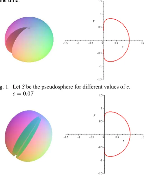
[image:3.595.314.563.452.756.2]

Fig. 1. Let S be the pseudosphere for different values of c. 0.07

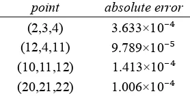
Fig. 2. Let S be the pseudosphere for different values of c.

0.055

IAENG International Journal of Applied Mathematics, 41:2, IJAM_41_2_04

(4)

For the radius of the pseudosphere we used the following formula:

1 2 /2 ² /2 ²

[image:4.595.357.496.168.238.2]

The following numerical results were obtained for the Dirichlet problem.

TABLE I: For 1, 0.055, 7, 16,

8 .

point absolute error

(2,3,4) 2.054×10⁻³

(12,4,11) 2.21×10⁻⁴

(10,11,12) 7.585×10⁻⁵

(20,21,22) 3.075×10⁻⁵

In all the examples we used the coefficient (*).

TABLE II: For 1, 0.06, 7, 16,

8 .

(2,3,4) 2.306×10⁻³

(12,4,11) 2.97×10⁻⁴

(10,11,12) 4.749×10⁻⁵

(20,21,22) 4.368×10⁻⁵

When we added 10 terms from the series (in the above tables only 5 terms were added from the series), we obtained the following TABLE III.

TABLE III: For 1, 0.055, 7,

16, 8 .

(2,3,4) 2.05×10⁻³

(12,4,11) 2.193×10⁻⁴

(10,11,12) 7.403×10⁻⁵

(20,21,22) 3.144×10⁻⁵

[image:4.595.103.244.322.394.2]

As you can see from the above TABLE III and the results were mostly better compared to the TABLE I. Now we increased the integration nodes, and obtained the following table.

TABLE IV: For 1, 0.055, 7,

32, 8 .

(2,3,4) 1.945×10⁻³

(12,4,11) 2.193×10⁻⁴

(10,11,12) 2.193×10⁻⁵

(20,21,22) 4.535×10⁻⁵

We can see from the above table that when you increase the integration nodes, the accuracy improves. Thus we can add more than five terms and still obtain good results if we

increase the number of integration nodes. But as more terms and increasing of integration nodes, increases the CPU time considerably (this will be discussed later more extensively), we added only a few terms, only five in other cases of pseudosphere. In the next table we changed the wave number k.

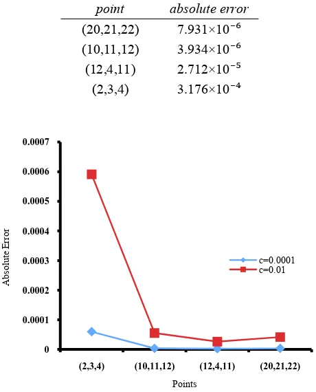
TABLE V: For 0.01, 0.005, 7,

16, 8 .

(2,3,4) 3.633×10⁻⁴

(12,4,11) 9.789×10⁻⁵

(10,11,12) 1.413×10⁻⁴

(20,21,22) 1.006×10⁻⁴

From the above tables, we see that for the points away from the boundary there is much greater accuracy than for points near the boundary. This is because the integrand is more singular at points near the boundary. We use NINTI = 16 in calculating the Galerkin coefficients , . The errors are printed in the column absolute error.

TABLE VI: For 5, 0.005, 7,

16, 8 .

(2,3,4) 1.814×10⁻²

(12,4,11) 2.075×10⁻³

(10,11,12) 9.00×10⁻⁴

(20,21,22) 1.632×10⁻⁴

From the above tables we see that to obtain similar accuracy as in the previous tables we might need to increase the integration nodes. This is due to the following fact: the

kernel function involves sin and cos , and these

trigonometric functions are much more oscillatory when k

becomes large. Therefore in this case we must increase the integration nodes to achieve the same accuracy.

Remark:

We picked , because the integrand of

, is smoother than the integrand of . We also

picked 1 . Now we changed to the

Neumann condition and the following tables are for the Neumann problem.

TABLE VII: For 1, 0.001, 7,

32, 16 .

(20,21,22) 3.646×10⁻⁶

(10,11,12) 3.748×10⁻⁶

(12,4,11) 2.537×10⁻⁶

(2,3,4) 5.987×10⁻⁵

IAENG International Journal of Applied Mathematics, 41:2, IJAM_41_2_04

[image:4.595.98.239.488.559.2] [image:4.595.98.239.664.735.2]

(5)

[image:5.595.52.282.86.371.2]

TABLE VIII: For k = 1, c = 0.01, NDEG = 7, NINTI = 32, NINTE = 16 andtrue solution u .

(20,21,22) 7.931×10⁻⁶

(10,11,12) 3.934×10⁻⁶

(12,4,11) 2.712×10⁻⁵

(2,3,4) 3.176×10⁻⁴

Fig. 3. Absolute Error at k = 1.

When c is changed, we obtained new shapes of

[image:5.595.356.497.87.158.2]

pseudospheres. When we increased the nodes we obtained better results for relatively larger c values.

TABLE IX: For k = 5, c = 0.001, NDEG = 7, NINTI = 32, NINTE = 16 and true solution u .

(16,18,20) 6.87×10⁻⁶

(10,11,12) 7.593×10⁻⁶

(5,6,7) 4.875×10⁻⁵

(2,3,4) 3.393×10⁻⁴

[image:5.595.46.549.459.761.2]

Fig. 4. Absolute Error at k = 5.

TABLE X: For k = 1, c = 0.01, NDEG = 7, NINTI = 32, NINTE = 16 andtrue solution u .

(20,21,22) 4.175×10⁻⁵

(10,11,12) 4.545×10⁻⁵

(12,4,11) 2.641×10⁻⁵

(2,3,4) 5.912×10⁻⁴

As you see in the above two tables, still the accuracy is quite good for the two different pseudospheres.

Final Remarks:

Few terms from the infinite series were added in all our numerical experiments. This is because in numerical calculations it is inefficient to add the full series. So we allow only a finite number of the coefficients anm to be

different from zero.

[image:5.595.306.554.459.747.2]

According to Jones [8], this is sufficient to ensure uniqueness for the modified integral equations in a finite range of wave numbers k. In practical applications, one is usually concerned with a finite range of k so this is not a serious draw back. In order to use a large amount of nodes we need a considerably high amount of CPU time. From the above examples, we see that the error is affected by the boundary S, NINTI, NINTE, boundary data and k and c. As the value of the c decreases the hyperbolic nature of the pseudosphere for the Dirichlet problem increases and the rate of convergence decreases. See table XI.

TABLE XI: For k = 1, NDEG = 7, NINTI = 8, NINTE = 16 andtrue solution u .

point c = 1 c = 0.001 c = 0.00001

(2,3,4) 3.46E-01 5.73E-04 9.10E-06 (5,6,7) 1.50E-01 1.91E-04 3.22E-06 (10,11,12) 6.90E-02 1.06E-04 1.79E-06

(25,26,27) 2.82E-02 4.26E-05 6.41E-07

(50,53,54) 1.45E-02 2.26E-05 4.09E-07

Fig. 5. Absolute Error for varying c.

0 0.0001 0.0002 0.0003 0.0004 0.0005 0.0006 0.0007

(2,3,4) (10,11,12) (12,4,11) (20,21,22)

A

bsolute

E

rror

Points

c=0.0001 c=0.01

0.00E+00 5.00E-02 1.00E-01 1.50E-01 2.00E-01 2.50E-01 3.00E-01 3.50E-01 4.00E-01

(1,2,3) (5,6,7) (10,11,12) (25,26,30) (50,53,54)

c=1 c=0.001 c=0.00001

0 0.00005 0.0001 0.00015 0.0002 0.00025 0.0003 0.00035 0.0004

(2,3,4) (5,6,7) (10,11,12) (16,18,20)

A

bsolute

E

rror

Points

c=0.001

IAENG International Journal of Applied Mathematics, 41:2, IJAM_41_2_04

[image:5.595.50.271.476.760.2]

(6)

This is not surprising considering that anmoriginally defined

by Jones for a constant radius R.

The role of k is more significant for ill-behaved boundary shapes. If we want to obtain more accuracy, we must increase the number of integration nodes for calculating the Galerkin coefficients , . The cost of calculating the Galerkin coefficients is high.

Some of the increased cost comes from the complex number calculations, which is an intrinsic property of the Helmholtz equation. Furthermore any integration method is affected by k, due to the oscillatory behavior of the fundamental solution . Also the CPU time depends on the number of terms added from the series.

In order to eliminate more interior Neumann and Dirichlet eigenvalues we need a more powerful computer which would decrease the CPU time considerably. We also see that for the shapes of pseudosphere with small c values the convergence results are quite good, even though the coefficient choice that was used was originally designed for spherical regions.

ACKNOWLEDGMENT

We would like to thank Dr. Rutherford and Mrs. Kennedy for their technical support in getting this paper ready.

REFERENCES

[1] K. E. Atkinson, “The numerical solution of the Laplace's equation in three dimensions”, SIAM J. Numer. Anal., 19, (1982), pp. 263-274.

[2] K. E. Atkinson, “The numerical solution of integral equations of the second kind”, Cambridge University

Press, 1998.

[3] N. L. Balazs and A. Voros, “Chaos on the pseudosphere”, Service de Physique Théorique,

CEN-Saclay, 91191 Gif-sur-Yvette Cedex, France, 2002. [4] A. J. Burton, “The solution of Helmholtz' equation in

exterior domains using integral equations”, Division of Numerical Analysis and Computing, Teddington,

Middlesex, NPL report NAC 30, 1973.

[5] Howard Cohl, “Closed form expansions and Fourier expansions for the fundamental solution of Laplace's equation in the hyperbolic geometry”, Atlas: New Zealand Mathematics Colloquim, 2009, Auckland, New Zealand.

[6] David Colton and Rainer Kress, “Integral equation methods in scattering theory”, 1983.

[7] C. Criado and N. Alamo, “Thomas rotation and

Foucault pendulum under a simple unifying

geometrical point of view”, International Journal of Non-Linear Mechanics, 44, (2009), pp. 923-927. [8] D. S. Jones, “Integral equations for the exterior acoustic problem”, Q. J. Mech. Appl. Math. 27, (1974), pp. 142.

[9] G. Jost, “Integral equations with modified fundamental solution in time-harmonic electromagnetic scattering”,

IMA Journal of Applied Mathematics 40, (1988), pp. 129-143.

[10] R. E. Kleinman and R. Kress, “On the condition number of integral Equations in acoustics using

modified fundamental solutions”, IMA Journal of

Applied Mathematics, (1983), 31, pp. 79-90.

[11] R. E. Kleinman and G. F. Roach, “On modified Green functions in exterior problems for the Helmholtz

equation”, Proc. R. Soc. Lond. A 383, (1982), pp. 333.

[12] R. E. Kleinman and G. F. Roach, “Operators of minimal norm via modified Green's functions”, Proceedings of the Royal Society of Edinburgh, 94A, (1983), pp. 178.

[13] T. C. Lin, “The numerical solution of the Helmholtz equation using integral equations”, Ph.D. thesis, (July 1982), University of Iowa, Iowa City, Iowa.

[14] T. C. Lin, “The numerical solution of Helmholtz equation for the exterior Dirichlet problem in three dimensions”, SIAM, J. Numerical Anal., vol 22, No. 4,

(1985), pp. 670-686.

[15] T. C. Lin, “Smoothness results of single and double layer solutions of the Helmholtz equations”, Journal of Integral Equations and Applications, Vol.1, Number 1, (1988), pp. 83-121.

[16] T. C. Lin and Y. Warnapala-Yehiya, “The numerical solution of the exterior Dirichlet problem for

Helmholtz's equation via modified Green's functions

approach”, Computers and Mathematics with

Applications, Vol 44, (2002), pp. 1229-1248.

[17] F. Sausset and G. Tarius, “Periodic boundary conditions on the pseudosphere”, J. Phys. A: Mathematical and Theoretical, 40, (1983), 12873.

[18] Harry A. Schenk, “Improved integral formulation for acoustic radiation problems”, Journal of the Acoustical Society of America, (1967), pp. 41-58.

[19] F. Ursell, “On the exterior problems of acoustics”, II. Proc. Cambridge Phil. Soc. 84, (1978), pp. 545-548. [20] Y. Warnapala and E. Morgan, “The numerical solution of the exterior Dirichlet problem for Helmholtz's

equation via modified Green's functions approach for the oval of Cassini”, Far East Journal of Applied Mathematics, Vol 34, (2009), pp. 1-20.