Turbo Pascal Numerical Methods Toolbox 1986 pdf

(1)

(2)

-Turbo Pascal Numerical Methods Toolbox

Borland's No-Nonsense License Statement!

This software is protected by both United States copyright law and international treaty provisions. Therefore, you must treat this software just like Q book, with the following single exception. Borland International authorizes you to make archival copies of the software for the sole purpose of backing-up our software and protecting your investment from loss.

By saying, "just like a book," Borland means, for example, that this software may be used by any number of people and may be freely moved from one computer location to another, so long as there is no possibility of it being used at one location while it's being used at another. Just like a book that can't be read by two different people in two different places at the same time, neither can the software be used by two different people in two different places at the same time. (Unless, of course, Borland's copyright has been violated.)

Borland International grants you (the licensed owner of the Turbo Pascal Numerical Toolbox) the right to incorporate toolbox routines into your programs. You may distribute your programs that contain Numerical Toolbox routines in executable form without restriction or fee, but you may not give away or sell any part of the actual Numerical Methods Toolbox source code. You are not, of course, restricted from distributing your own source code.

Sample programs are provided on the Numerical Methods Toolbox diskettes as examples of how to use the various toolbox features. You may edit or modify these sample programs and incorporate them into the programs that you write. Use of these sample programs is governed by the same conditions and restrictions as outlined in the first paragraph above.

WARRANTY

With respect to the physical diskette and physical documentation enclosed herein, Borland International, Inc. ("Borland") warrants the same to be free of defects in materials and workmanship for a period.of 60 days from the date of purchase. In the event of notification within the warranty period of defects in material or workman-ship, Borland will replace the defective diskette or documentation. If you need to return a product. call the Borland Customer Service Department to obtain a return authorization number. The remedy for breach of this warranty shall be limited to replacement and shall not encompass any other damages, including but not limited to loss of profit, and special, incidental, consequential, or other similar claims.

Borland International, Inc. specifically disclaims all other warranties, expressed or implied, including but not limited to implied warranties of merchantability and fitness for a particular purpose with respect to defects in the diskette and documentation, and the program license granted herein in particular, and without limiting operation of the program license with respect to any particular application, use, or purpose. In no event shall Borland be liable for any loss of profit or any other commercial damage, including but not limited to special, incidental, consequential or other damages.

(3)

Turbo Pascal

Numerical

Methods

Toolbox~

(4)

(5)

Table of Contents

Introduction ... 1

Toolbox Functions ... 1

About this Manual ... 2

On the Distribution Disks ... 3

System Requirements ... 3

Acknowledgements ... 4

Chapter 1. ROUTINE BEGINNINGS ... 5

Using the Toolbox: An Example ... 5

The Distribution Disks ... 7

Installation ... 8

The Graphics Demos ... 12

Data Types and Defined Constants ... 12

Compiler Directives ... 13

Chapter 2. ROOTS TO EQUATIONS IN ONE VARIABLE ... 15

Stopping Criteria ... 17

Root of a Function Using the Bisection Method (BISECT.lNC) ... 18

Description ... 18

User-Defined Function ... 18

Input Parameters ... 18

Output Parameters ... 19

(6)

Comments ... 19

Sample Program ... 19

Example ... 20

Root of a Function Using the Newton-Raphson Method (RAPHSON.lNC) ... 21

Description ... 21

User-Defined Functions ... 21

Syntax of the Procedure Call ... 22

Comments ... 22

Example ... 23

Root of a Function Using the Secant Method (SECANT.lNC) ... 25

Description ... 25

Comments ... : ... 26

Example ... 27

Real Roots of a Real Polynomial Equation Using the Newton-Horner Method with Deflation (NEWTDEFL.lNC) ... 28

Description ... 28

User-Defined Types ... 28

Comments ... 30

Input Files ... 30

Example ... 30

Complex Roots of a Complex Function Using Miiller's Method (MULLER.INC) ... 33

Description ... 33

User-Defined Procedure ... 33

(7)

Complex Roots of a Complex Polynomial Using Laguerre's Method and Deflation

(LAGUERRE.INC) ... 37

Description ... 37

Comments ... 38

Input Files ... 39

Example ... 39

Chapter 3. INTERPOLXfION ... 43

Polynomial Interpolation Using Lagrange's Method (LAGRANGE.lNC) ... .45

Description ... 45

Input Files ... 46

Example ... 47

Interpolation Using Newton's Interpolary Divided-Difference Method (DIVDIF.INC) ... 49

Description ... 49

Output Parameters ...

90

Input Files ... 50

Example ... 50

Free Cubic Spline Interpolation (CUBE-FRE.lNC) .: ... 52

Description ... 52

Syn tax of the Procedure Call ... 53

Input Files ... 54

Example ... 54

Clamped Cubic Spline Interpolation (CUBE_CLA.lNC) ... 57

Description ... 57

(8)

Input Files ... 59

Example ... 59

Chapter 4. NUMERICAL DIFFERENTIATION ... 63

First Differentiation Using Two-Point, Three-Point, or Five-Point Formulas (DERIV.INC) ... 66

Description ... 66

Comments ... 67

Input Files ... 68

Example ... 68

Second Differentiation Using Three-Point or Five-Point Formulas (DERIV2.INC) ... 71

Description ... 71

Comments ... 72

Input Files ... 73

Example ... 73

Differentiation with a Cubic Spline Interpolant (INTERDRV.lNC) ... 76

Description ... 76

User-Defined Types .: ... 76

Syntax of the Pn;)cedure Call ... 77

(9)

Comments ... 81

Input Files ... 81

Example ... 82

Second Differentiation of a User-Defined Function (DERIV2FN.INC) ... 83

Description ... 83

User-Defined Function ... ; ... 83

Comments ... 84

Input Files ... 85

Example ... 85

Chapter 5. NUMERICAL INTEGRATION ... 87

Integration Using Simpson's Composite Algorithm (SIMPSON.INC) ... 89

Description ... 89

Example ... 90

Integration Using the Trapezoid Composite Rule (TRAPZOID.INC) ... 92

Description ... 92

Example ... 93

Integration Using Adaptive Quadrature and Simpson's Rule (ADAPSIMP.INC) ... 95

Description ... 95

Comments ... 96

(10)

Example ... 97

Integration Using Adaptive Quadrature and Gaussian Quadrature (ADAPGAUS.INC) ... 98

Description ... 98

Comments ... 99

Example ... 101

Integration Using the Romberg Algorithm (ROMBERG.INC) ... 102

Description ... 102

Example ... 103

Chapter 6. MATRIX ROUTINES ... 105

Determinant of a Matrix (DET.INC) ... 107

Description ... 107

Input File ... 108

Example ... 109

Inverse of a Matrix (INVERSE.INC) ... 110

Description ... 110

User-Defined Types ... ; ... 110

(11)

Input File ... 115

Example ... 116

Solving a System of Linear Equations with Gaussian Elimination and Partial Pivoting (PARTPIVI'.1 N C) ... 117

Description ... 117

Syntax of the Procedure Call ... : ... 118

Input File ... 118

Example ... 119

Solving a System of Linear Equations with Direct Factoring (DIRFACT.INC) ... 120

Description ... 120

Procedure LU-Decompose Input Parameters ... 121

Procedure LU-Decompose Output Parameters ... 121

Procedure LU_Solve Input Parameters ... 121

Procedure LU_Solve Output Parameters ... 122

Input File ... 122

Example ... 123

Solving a System of Linear Equations with the Iterative Gauss-Seidel Method (GAUSSIDL.INC) ... 126

Description ... 126

Input File ... 128

Example ... 129

Chapter 7. EIGENVALUES AND EIGENVECTORS ... 131

Real Dominant Eigenvalue and Eigenvector of a Real Matrix Using the Power Method (POWER.INC) ... 133

Description ... 133

(12)

Comments ... 134

Input File ... 135

Example ... 135

Real Eigenvalue and Eigenvector of a Real Matrix Using the Inverse Power Method (INVPOWER.INC) ... 137

Description ... 137

Comments ... 139

Input File ... 139

Example ... 140

Real Eigenvalues and Eigenvectors of a Real Matrix Using the Power Method and Wielandt's Deflation (WIELANDT.lNC) ... 143

Description ... 143

Comments ... 145

Input File ... 146

Example ... 146

The Complete Eigensystem of a Symmetric Real Matrix Using the Cyclic Jacobi Method (JACOBI.INC) ... 149

Description ... 149

Comments ... 151

(13)

Description ... 159

Comments ... 161

Example ... 162

Solution to an Initial Value Problem for a First-Order Ordinary Differential Equation Using the Runge-Kutta-Fehlberg Method (RKF_1.1NC) ... 163

Description ... , ... 163

User-Defined Types ... : ... 163

Comments ... 165

Example ... 166

Solution to an Initial Value Problem for a First-Order Ordinary Differential Equation Using the Adams-Bashforth/Adams-Moulton Predictor/Corrector Scheme (ADAMS_l.INC) ... 168

Description ... 168

Comments ... 170

Sample Program ... : ... 170

Example ... 171

Solution to an Initial Value Problem for a Second-Order Ordinary Differential Equation Using the Runge-Kutta Method (RUNGE-2.1NC) ... 172

Description ... 172

Syntax of the Procedure Call ... : ... 174

Comments ... ; ... 174

Example ... 175

(14)

Solution to an Initial Value Problem for an nth-Order Ordinary Differential

Equation Using the Runge-Kutta Method (RUNGE_N.lNC) ... 178

Description ... 178

Comments ... 181

Example ... 182

Solution to an Initial Value Problem for a System of Coupled First-Order Ordinary Differential Equations Using the Runge-Kutta Method (RUNGE_Sl.INC) ... 186

Description ... ; ... 186

User-Defined Types .: ... 188

Comments ... 190

Example ... 191

Solution to an Initial Value Problem for a System of Coupled Second-Order Ordinary Differential Equations Using the Runge-Kutta Method (RUNGE_S2.INC) ... 196

Description ... 196

Comments ... 201

Example ... 203

Solution to Boundary Value Problem for a Second-Order Ordinary Differential Equation Using the Shooting and Runge-Kutta Methods (SHOOT2.1NC) .. 208

(15)

Example ... 211

Solution to a Boundary Value Problem for a Second-Order Ordinary Linear Differential Equation Using the Linear Shooting and Runge-Kutta Methods (LINSHOT2.INC) ... 215

Description ... 215

Comments ... 217

Example ... 218

Chapter 9. LEAST.SQUARES APPROXIMATION ... 221

Least-Squares Approximation (LEAST.lNC) ... 222

Description ... 222

Comments ... 224

POLY.LSQ ... 224

FOURIER.LSQ ... 225

POWER.LSQ ... 225

EXP.LSQ ... 225

LOG.LSQ ... 226

USER.LSQ ... 226

Input Files ... 227

Example ... 227

Chapter 10. FAST FOURIER TRANSFORM ROUTINES ... 233

The Application Programs ... 235

Data Sampling ... 239

Fast Fourier Transform Algorithms ... : ... 241

Procedure TestInput ... 241

Description ... 241

Procedure MakeSinCosTable ... 242

(16)

Description ... 242

Procedure FFT ... 242

Description ... 242

Fast Fourier Transform Applications ... 244

COMPFFT.INC ... 244

Description ... 244

Comments ... 245

REALFFT.INC ... 245

Description ... 245

Comments ... 246

COMPCNVL.INC ... 246

Description ... 246

Comments ... 247

REALCNVL.INC ... 248

Description ... 248

Comments ... 249

COMPCORR.INC ... 249

Description ... 249

(17)

Comments ... 252

Input File ... 253

Example ... 253

Chapter 11. GRAPHICS PROGRAMS ... 261

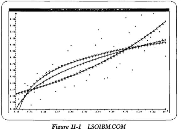
Function of the Least-Squares Graphics Demonstration Program ... 262

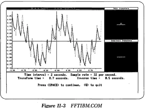
Function of the Fourier Transform Graphics Demonstration Program ... 264

Printing ... 265

Rebuilding LSQIBM.COM ... 267

Rebuilding FFTIBM.COM ... 268

Rebuilding for the Hercules Card ... 269

Rebuilding for the EGA Card ... 269

Using the Math Coprocessor ... 270

REFERENCES ... 271

INDEX ... 273

(18)

(19)

I

ntroductian

The Turbo Numerical Methods Toolbox is a reference manual for both the student of numerical analysis and the professional needing efficient routines. An elemen-tary background in calculus and linear algebra is assumed, although many of the algorithms use only high-school-level mathematics. A general knowledge of Turbo Pascal® is also assumed. If you need to brush up on your knowledge of Pascal, we suggest looking at the Turbo Pascal Reference Manual and/or the Turbo Pascal

Tutor Manual.

Before you begin using a particular routine, read through this brief introductory chapter and then refer to the chapter that interests you.

Toolbox

Functions

The Turbo Pascal Numerical Methods Toolbox provides routines for

• Finding solutions to equations

• Interpolations

• Calculus

• l'iumerical derivatives and integrals

(20)

• Differential equations

• Least-squares approximations

• Fourier transforms

About this Manual

The major areas in numerical analysis are represented in this Toolbox, with each chapter focusing on a particular problem. Each routine begins with a general description of the implemented algorithm or numerical method. (References to numerical analysis texts are provided for each numerical procedure.) User-supplied types, functions, and input and output parameters are defined, and the syntax of the procedure call is provided. If appropriate, a "Comments" section is also pro-vided.

Finally, every algorithm in the Toolbox is accompanied by a general-purpose program that handles all the necessary I/O, while allowing you to try each algo-rithm without building any code. Handily, these sample programs will often reduce the coding your own application may require.

As an example, let's say you want to find the roots to an equation in one variable. First, you would read the introduction to Chapter 2, "Roots to Equations in One Variable," and choose the numerical method best suited to your particular problem. Second, you would run the sample program for the desired numerical method to determine the necessary input and output. Third, you would write a Turbo Pascal function defining your equation, using the function already coded in the sample program as a guide. Fourth, you would run the sample program with your function substituted for the original one. Of course, if these algorithms are to be part of a larger program, you must build all the interfaces to the other parts of the system; but this should only be done after you gain experience with the particular numeri-cal method.

Several books are referred to throughout the text; complete references are listed at the back of the book in the section entitled "References."

The body of this manual is printed in normal typeface; other typefaces serve to illustrate the following:

(21)

On the Distribution Disks

The routines for this Toolbox are contained on three packed disks. Their contents and general installation instructions are covered in Chapter l.

System Requirements

All routines will run in standard Turbo Pascal version 3.0. (They will also run in version 2.0, but you must make one change to use the sample programs; see the section entitled "Installation" in Chapter 1.) All sample programs will run on an IBM® PC or compatible machine using DOS 2.0 or greater.

A small portion of the Toolbox uses graphics (see Chapter 11). These programs are for PC-DOS users only, requiring either an IBM PC Color Graphics Adapter, an IBM Enhanced Graphics Adapter, or a Hercules Monochrome Graphics Adapter. Recompiling these requires the Turbo Pascal Graphix Toolbox® version 1.06A or later, and Turbo Pascal 3.0. They can also be recompiled for the EGA and several other cards using version 1.07 A of the Graphix Toolbox.

We strongly recommend that anyone serious about numerical analysis invest in hardware and software to run Turbo Pascal with support for the Intel 8087 numeri-cal processing chip:

• Hardware: an 8087 chip plugged into the motherboard of a PC, XT® or equiva-lent, or an 80287 chip in an AT® or equivalent.

• Software: TURBO-87.COM, the version of Turbo Pascal designed to take advan-tage of the 8087 chip.

For machines running the Intel 8088 CPU, the increase in execution speed of programs using real-number arithmetic is often a factor of ten or more, while for 80286 machines, the increase is only about a factor of two (Fried 1985). Perhaps more important than speed is the increase in accuracy -16 significant figures accu-racy for Turbo Pascal with 8087 support versus 11 significant figures for standard Turbo. Since round-off errors are a serious concern in numerical analysis, the increased accuracy is of great value.

All of the examples in this manual were run using Turbo-87. If you run them without the Turbo-87, you will usually get less accurate answers.

(22)

AcktWwlellgements

We refer to several products throughout the manual; following is a list of each one and its respective company.

• Turbo Pascal, Turbo Pascal Graphix Toolbox, SideKick, SuperKey, and Reflex: The Database Manager are registered trademarks and Turbo Pascal Numerical Methods Toolbox is a trademark of Borland International, Inc.

• IBM, XT, and AT are registered trademarks of International Business Machines Corp.

(23)

c

H A p T E R

1

Routine Beginnings

This chapter provides you with everything you need to start using the routines in this Toolbox. We'll discuss how to unpack the disks for use and list the files avail-able once the disks are unpacked. We also briefly discuss data types and defined constants used in the Toolbox, and the setting of compiler directives.

First, though, before we thrust you into the middle of numerical madness, let's take a look at one way to use this Toolbox.

Using

the

Toolbox: An Example

In late 1986 and early 1987, the America's Cup 12-meter yacht championship was held. The 12-meter yachts are just large sailboats, but the competition is so intense that the only way to be competitive is to use dozens of people, spend millions of dollars, design a special boat, and spend a couple of years training for the race. The race has become so sophisticated that many of the sailboats have on-board com-puters and other electronic equipment.

To keep stride with other challengers, one yacht's crew used personal com-puters, and of course, Borland software. They used Turbo Pascal to design the boat's hull. They used Reflex: The Analyst® to maintain their databases and to dis-play plots while the boat was sailing. And when it came time to do some mathemat-ical modeling, again they turned to Borland for its inimitable software and chose the Toolbox.

(24)

Simply speaking, the problem they had was one of "precision monitoring." It takes a crew of very highly skilled sailors to compete in America's Cup races, but even the best skippers cannot act with sufficient precision to win. A typical race lasts for several hours, and the winner usually wins by only a few feet.

The electronic equipment on a boat can sense with reasonable accuracy all of the crucial variables: boat velocity, wind velocity, boat direction, boat position, and so on. This data must then be made available to the skipper in a coherent form, and he/she must decide at what angle to place the rudder based on that information. The problem is too complex to rely on intuition alone.

Even just displaying the velocity is more complex than you might think at first. When sailing on the ocean, the waves are big enough that the velocity is in constant flux. Fortunately, the fluctuations due to the waves represents a steadily periodic force. By using the Fourier transforms in Chapter 10 of the Toolbox, the crew was able to identify the periodic portion of the velocity and subtract it out. The result: the velocity as a function of time but with the wave fluctuations eliminated. The graph of this modified velocity is much smoother, and allows the skipper to tell much more quickly and accurately whether the boat is accelerating or decelerating.

To measure the acceleration quantitatively, the crew used the fact that the accel-eration is the derivative of the velocity. They were able to do this easily with the

differentiation routines in Chapter 4 of the Toolbox. They were also able to directly measure the distance travelled by using the integration routines in Chapter 5, and the fact that distance is the integral of the speed.

Perhaps the most difficult problem in navigating a sailboat is aiming the rudder. You can't just aim the boat in the direction that you want to go, rather you have to pick a direction that you can sail rapidly, depending on the wind direction. An experienced skipper can judge this pretty well, but not well enough. Every boat is a little different, and the best way to handle one boat is not necessarily the best way to handle another.

So, the team ran extensive trial races with the boat to gather data on how the boat performed in various circumstances. The data was collected automatically by electronic instruments on board, and stored digitally on floppy disks. They then used Reflex to manage the data and to display graphs. But they lacked the tools to relate their data to the data they would have under actual racing conditions.

(25)

This, of course, is just one of many applications of this Toolbox. Now, let's go on to the fundamentals.

. The Distribution Disks

All of the Toolbox routines are contained on three disks. (Note, however, that MS-DOS® users will receive two disks; Disk 3 is for PC-DOS users only.) Each disk has packed files corresponding to chapters in the manual. Use the program UNPACK.EXE to unpack the files, described in the next section, "Installation."

The files for each chapter are self-contained and do not require any files from any other chapter, with these exceptions:

\

• All files require Turbo Pascal (not included).

• Most files require COMMON.INC, located on Disk l.

• The files for Chapter 11 require files from Chapters 9 and 10, as well as the Turbo Pascal Craphix Toolbox (not included).

The numerical analysis routines are in the files with the .INC suffix. The files with the .PAS suffix are demonstration programs. To run a demonstration program, get into Turbo Pascal and load the .PAS file of your choice. The menus are self-explanatory. The .DAT files contain input data for specific .PAS files.

If you're a PC-DOS user with an IBM color graphics monitor or compatible, you can run LSQIBM.COM or FFfIBM.COM from Disk 3 to see a quick graphic demonstration of the power and usefulness of the Toolbox. These routines require the files SAMP11A.DAT, SAMPllB.DAT, 4X6.FON, 8X8.FON, and ERROR.MSC to be on the current directory. (These files are also on Disk 3.)

Contents of the enclosed disks:

Disk 1 README

README.COM (program to display README file) UNPACK.EXE (installation program to unpack chapters) COMMON.INC (used throughout the Toolbox)

COMMON2.INC (for Turbo Pascal 2.0 users) CHAP2 (packed file with routines for Chapter 2) CHAP3 (packed file with routines for Chapter 3) CHAP4 (packed file with routines for Chapter 4) CHAP5 (packed file with routines for Chapter 5) CHAP6 (packed file with routines for Chapter 6) CHAP7 (packed file with routines for Chapter 7)

(26)

Disk 2

UNPACK.EXE (installation program to unpack chapters) CHAP8 (packed file with routines for Chapter 8)

CHApg (packed file with routines for Chapter 9) CHAPIO (packed file with routines for Chapter 10)

CHAP11 (packed file with routines for Chapter 11; PC-DOS users only)

Disk 3 (PC-DOS users only) README

README.COM (program to display README file) LSQIBM.COM (requires IBM graphics monitor) FFTIBM.COM (requires IBM graphics monitor) LSQHERC.COM (requires Hercules graphics card) FFTHERC.COM (requires Hercules graphics card) SAMP11A.DAT (data file for LSQ*.COM)

SAMP11B.DAT (data file for FFT*.COM) 14X9.FON (from the Graphix Toolbox) 4X6.FON (from the Graphix Toolbox) 8X8.FON (from the Graphix Toolbox) ERROR.MSG (from the Graphix Toolbox)

Installation

The files CHAP2 through CHAP11 are packed files corresponding to the chapters in this manual. In order to use these files, you must first unpack them with UNPACK.EXE. The syntax is as follows:

UNPACK packed-file-name target-drive

For example, the files for Chapter 2 can be extracted and put on the current directory on drive C by placing Disk 1 in drive A, changing the logged drive to A by typing A: at the DOS prompt, and then typing

UNPACK CHAP2

c:

(27)

You may wish to copy the packed files onto your hard disk, and then unpack them as you need them.

Note: These files are not copy protected. All files are ordinary DOS files; there are no hidden files. The unpacking program only extracts ordinary text files - it will not create directories, modify the distribution disk, create hidden or protected files, or do anything unexpected.

Contents of the packed files:

CHAP2 (packed file)

BISECT.lNC

BISECT.PAS

LAGUERRE.lNC

LAGUE RRE. PAS

MULLER.lNC

MULLERPAS

NEWTDEFL.lNC

CHAP3 (packed file)

CUBE_CLA.lNC

CUBE_CLAPAS

CUBE-FRE.lNC

CUBE_FRE.PAS

DIVDIF.INC

DIVDI F. PAS

LAGRANGE.lNC

LAGRANGE. PAS

SAMPLE3A.DAT

CHAP4 (packed file)

DERIV.lNC DERIV.PAS DERIV2.1NC DERIV2.PAS DERIVFN.lNC DERIVFN.PAS

Routine Beginnings

"Roots to Equation in One Variable"

N EWTDEFL. PAS

(28)

CHAP5 (packed file) ADAPGAUS.lNC ADAPGAUS.PAS ADAPSIMP.lNC ADAPSIMP.PAS ROMBERG.INC

CHAP6 (packed file)

DET.INC DET.PAS DIRFACT.INC DIRFACT.PAS GAUSELIM.INC GAUSELIM.PAS GAUSSIDL.INC GAUSSIDL.PAS

CHAP7 (packed file)

INVPOWER.INC INVPOWERPAS JACOBI.INC JACOBI. PAS POWER.INC "Numerical Integration" ROMBERG.PAS SIMPSON.lNC SIMPSON.PAS TRAPZOID.lNC TRAPZOID.PAS "Matrix Routines" INVERSE.INC INVERSE.PAS PARTPIVT.INC PARTPIVT.PAS SAMPLE6A.DAT SAMPLE6B.DAT SAMPLE6C.DAT SAMPLE6D.DAT

"Eigenvalues and Eigenvectors"

POWERPAS

SAMPLE7 ADAT

WIELANDT.lNC

WIELANDT.PAS

CHAPS (packed file) "Initial Value and Boundary Value Methods"

ADAMS_l.INC RUNGE-2.PAS

ADAM S_I. PAS

LINSHOT2.1NC

LINSHOT2.PAS

RKF_l.INC

RKF_l.PAS .

RUNGE_N.INC

RUNGE-N.PAS

RUNGE_Sl.INC

RUNGE_Sl.PAS

(29)

CHAP9 (packed file) EXP.LSQ FOURIERLSQ LEAST.INC LEAST. PAS LOG.LSQ

CHAPIO (packed file)

COMPCNVL.INC COMPCORRINC COMPFFT.INC FFT87B2.INC FFT87B4.INC FFTB2.INC FFTB4.INC "Least-Squares Approximations" POLY.LSQ POWERLSQ SAMPLE9A.DAT USERLSQ

"Fast Fourier Transform Routines"

FFTPROGS.PAS REALCNVL.INC REALCORR.INC REALFFT.IN C SAMPIOA.DAT SAMPI0B.DAT SAMPIOC.DAT

CHAPll (packed file) "Graphics Programs" IPC-DOS only

FFTDEMO.PAS LEAST.MOD

GENERIC.LSQ

GRAPHIX.EGA

GRAPHIX.HGC

IOCHECK.INC

LSQDEMO.PAS

All sample programs call the include file COMMON.INC from the disk. This file includes procedures that are common to all sample programs. When copying any of the sample programs to a disk, be sure to also copy the file COMMON.INC to that disk or the sample programs will not compile.

To use the sample programs with Turbo Pascal version 2.0, rename COM-MON2.INC (which is on Disk 1) to COMMON.INC. (You may wish to preserve a copy of tlie original COMMON.INC file by first copying it to a file called COM-MON3.INC). If you run the sample programs with version 2.0 and do not make this change, the programs will compile but will handle I/O errors incorrectly.

We have made the sample programs general and easy to use. For example, numerical input can originate from the keyboard (where improper input is trap-ped) or from a text file; output can be sent to the printer, screen, or text file; other refinements are also included. Since, to a beginner, the supporting code may obscure the simplicity of calling the procedure, we have included a minimal sample program for Newton-Raphson's method of root-finding (RAPHSON2.INC).

(30)

The Graphics Denws

Because graphic displays are often an essential part of numerical analysis, we have included two demonstration programs (for PC-DOS users only) that involve dis-play numerical results. As previously stated, graphics hardware is not necessary for this Toolbox, but it is required for these two graphics programs. The programs are built with subsets of the Turbo Pascal Graphix Toolbox; there are separate versions for systems with the Hercules Monochrome Graphics card and the IBM Color Graphics card (or good emulations of these cards).

The demonstration programs are on Disk 3. For instructions about how to run or recompile them, see Chapter 11.

Data Types and Defined Constants

Data types that might be confused with those in the calling program have been prefixed with the letters TN (for Turbo Numerical); for example, TNmatrix or

TN vector. You must define these variable types in your top-level program for two reasons. First, you will probably need to use this type in your top-level program, and the type must be defined to have the same scope as the Toolbox procedure. Second, you will want to dimension arrays based on your particular needs. For example, the Lagrange procedure requires the definition

type TNvector = array[O .. TNArraySize] of Real;

The identifier TNArraySize is never referred to in any of the include files. It should be optimized by the user, although we have set a default value in each of the sample programs. It may be replaced with an integer or byte.

(31)

Compiler Directives

Aside from the usual default values of the compiler directives in standard Turbo Pascal, we have set the compiler directive to {$R

+ }

in all include files that use arrays, and to {$I-} in all sample programs. The first directive checks to see that all array-indexing operations are within the defined bounds and all assignments to scalar and subrange variables are within range. The latter directive disables I/O error-checking. All the sample programs have their own I/O error-checking proce-dures (loaded in the file COMMON.lNC), so that the {$I-} directive must remain disabled in the sample programs. The array checker {$R

+}

should always be active, since the performance penalty is slight and the advantages are significant.

(32)

(33)

c

H A p T E R

2

Roots to Equations in One Variable

The routines in this chapter are for finding the roots of a single equation in one real variable. A typical problem is to solve

x

*

exp(x) - 10 = 0 .

In general, the routines find a value of x, where x is a scalar real variable, satisfying

f(x) = 0.0

where

f

is a real-valued function that you program in Pascal.

All of the methods are approximate methods, meaning that they find an approxi-mate value of x that makesf(x) close to zero. Because of round-off error, it is usually not possible to find the exact value of x. Furthermore, they are all iterative methods, meaning that you specify some initial guess that is some value for x, which you think is reasonably close to the solution. The routine repeats some calcu-lations that replace the guess x with a more accurate guess until the required level of accuracy is achieved.

The bisection method (BISECT.INC) returns an approximation to a root of a real continuous function of the real variable x. This method always converges (as long as the function changes signs at a root), but may do so relatively slowly.

The Newton-Raphson method (RAPHSON.INC) also returns an approximation to a root of a real functionf of the real variable x. When this algorithm converges, it is usually faster than the bisection method. If more than one root of a polynomial equation is desired, then use Newton-Horner's method (NEWfDEFL.INC).

(34)

The secant method (SECANT.lNC) is similar to the Newton-Raphson method, but doesn't require knowledge of the first derivative of the function. Consequently, it is more flexible than the N ewton-Raphson method, though somewhat slower.

Newton-Horner's method (NEWfDEFL.lNC) applies Newton's method to real polynomials. It also uses deflation techniques to attempt to approximate all the real roots of a real polynomial. Both the Newton-Horner and Newton-Raphson methods are faster than the bisection and secant methods, but are undefined if

If'(x)1

<

=

TNNearlyZero. This is less of a problem on machines with a high-precision math coprocessor, since TNNearlyZero is smaller.

The Newton-Horner and Newton-Raphson methods both converge around mul-tiple roots, although convergence is slow. These algorithms depend upon an initial approximation of the root. If the initial approximation is not sufficiently close to the root, the Newton methods may not converge. In some instances, an initial choice may lead to successive iterations that oscillate indefinitely about a value of x usu-ally associated with a relative minimum or relative maximum off. In either case, the bisection method could be used to determine the root or to determine a close approximation to the root that can be employed as an initial approximation in the Newton-Raphson or Newton-Horner methods.

Muller's method (MULLER.lNC) returns an approximation to a root (possibly complex) of a complex function of the complex variable x. Although Muller's method can approximate the roots of polynomials, we recommend that you use Newton-Horner's method, the secant method, or (in the case of complex polyno-mials) Laguerre's method to find the roots of polynomials.

Laguerre's method (LAGUERRE.lNC) attempts to approximate all the real and complex roots of a real or complex polynomial. Laguerre's method is very reliable and quick, even when converging to a multiple root. This is the best general method to use with polynomials.

A caution when solving polynomial equations: Polynomials can be

(35)

Stopping Criteria

All the root-finding routines use the function TestForRoot to determine if a root has been found.

function TestForRoot{X, OldX, V, Tol : Real) : Boolean;

(********************************************************************) (* Here are four stopping criteria. If you wish to *) (* change the active criteria, simply comment off the current *) {* criteria (including the appropriate or) and remove the comment *) {* brackets from the criteria (including the appropriate or) you *)

(* wish to be active. *)

(********************************************************************)

begin

TestForRoot :=

(ABS{V) <= TNNearlyZero)

or

(ABS{X - OldX) < ABS{OldX*Tol))

{* or {*

{* (ABS{X - OldX) < Tol) {*

{* or {*

(* (ABS{V) <= Tol)

end; { procedure TestForRoot }

(***************************)

(* V=O *)

(* *)

(* relative change in X *)

(* *)

*) (* *)

*) (* absolute change in X *)

*) (* *)

*) (* absolute change in V *) (***************************)

The four separate tests provided by function TestForRoot may be used in any combination. The default criteria tests the absolute value of Y and the relative change in X. If you wish to change the active criteria, simply comment off the current criteria (including the appropriate or) and remove the comment brackets from the criteria (including the appropriate or) you wish to be active.

The first criterion simply checks to see if Y is zero (TNNearlyZero is defined at the beginning of the procedure). This criterion should usually be kept active.

The second criterion examines the relative change in X between iterations. To avoid division by zero errors, QldX has been multiplied through the inequality.

The third criterion checks the absolute change in X between iterations.

The fourth criterion determines the absolute difference between Y and the allowable tolerance. Note: The parameter Tol(erance) means something different in each test. Be sure you know which tests are active when you input a value for Tol.

(36)

Root of a Function Using the Bisection Method

(BISECT. INC)

Description

This method (Burden and Faires 1985, 28 ff.) provides a procedure for finding a root of a real continuous function

f,

specified by the user on a user-supplied real interval [a,b]. The functionsfia) and fib) must be of opposite signs. The algorithm successively bisects the interval and converges to the root of the function. You must also specify the desired accuracy to which the root should be approximated.

User- Defined Function

funct;on TNTargetF(x : Real) : Real;

The procedure Bisect determines the roots of this function.

Input Parameters

LeftEnd:Real; Left end of the interval

RightEnd:Real; Right end of the interval

To 1 : Rea 1 ; Indicates accuracy of solution

Maxlter:Real; Maximum number of iterations permitted

The preceding parameters must satisfy the following conditions:

1. LeftEnd < RightEnd.

2. TNTargetF(LeftEnd)

*

TNTargetF(RightEnd)

<

0; the endpoints must have opposite signs.

3. Tol > O.

(37)

Output Pararneters

Answer:Real; An approximate root of TNTargetF

fAnswer:Real; The value of the function at the value Answer

Iter: Integer; Number of iterations to find answer

Error:Byte; 0: No error 1: Iter > MaxIter

2: Endpoints are of the same sign

3: LeftErul > RightErul

4: Tol :::;; 0

5: MaxIter < 0

If Error = 1 (maximum number of iterations exceeded), Answer is set to the last

x value tested and fAnswer is set to TNTargetF(Answer). If Error> 1, then the other output parameters are not defined.

Syntax of the Procedure Call

Bisect(LeftEnd, RightEnd, Tol, MaxIter, Answer, fAnswer, Iter, Error);

The procedure Bisect determines the roots of function TNTargetF.

Comrnents

If a root occurs at a relative maximum or relative minimum, the bisection method will be unable to locate that value of p if P does not occur as an endpoint of a subinterval.

Convergence is determined with the Boolean function TestForRoot described at the beginning of this chapter.

Sample Program

The sample program BISECT.PAS provides I/O functions that demonstrate the bisection algorithm. To modify this program for your own function, simply change the definition of function TNTargetF. Note that the file BISECT.INC is included after the function TNTargetF is defined.

(38)

Example

Problem. Determine the solution to the equation cos(x)

=

x.

1. Write the following code for function TNTargetF into BISECT.PAS:

{--- HERE IS THE FUNCTION ---} funct;on TNTargetF(x : Real) : Real;

beg;n

TNTargetF := Cos (x) - x;

end; { function TNTargetF }

{---}

2. Run BISECT.PAS:

Left endpoint: 0 Right endpoint: 100

Tolerance (> 0, default = 1.000E-08): 1E-6

Maximum number of iterations (>= 0, default = 100)? 100 Direct output to one of the following:

(S)creen (P)rinter

(F) il e

Left endpoint: O.OOOOOOOOOOOOOOE+OOO Right endpoint: 1.00000000000000E+002 Tolerance: 1.00000000000000E-006 Maximum number of iterations: 100

Number of iterations: 28

Calculated root: 7.39085301756859E-001 Value of the function

(39)

Root of a Function Using the Newton-Haphson Method

(RAPHSON.INC)

Description

This example uses Newton-Raphson's algorithm (Burden and Faires 1985,42 fr.) to find a root of a real user-specified function when the derivative of the function and an initial guess are given. The algorithm constructs the tangent line at each iterate approximation of the root. The intersection of the tangent line with the x-axis provides the next iterate value of the root. You must specify the desired tolerance to which the root should be approximated.

User-Defined Functions

function TNTargetF(x : Real) : Real; function TNDerivF(x : Real) : Real;

The procedure Newton Raphson determines the roots of the function

TNTargetF.

The function TNDerivF must be the first derivative of function TNTargetF.

Input Parameters

Guess:Real; Tol:Real;

User's initial approximation to the root

Tolerance in answer (see "Comments")

MaxIter: Integer; Maximum number of iterations permitted The preceding parameters must satisfy the following conditions:

1. Tal> 0

2. MaxIter > 0

(40)

Output Parameters

Root: Rea 1 ; Approximate root.

Va 1 ue: Rea 1; Value of the function at the approximate root.

Deri v: Rea 1 ; Value of the derivative at the approximated root.

Iter: Integer; Number of iterations needed to find the root.

Error:Byte; 0: No error.

1: Iter < MaxIter.

2: The slope is zero (see "Comments").

3: Tol :$ O.

4: MaxIter < O.

If a root is found, it is returned along with the value of the function at the root (which, of course, should be close to zero) and the value of the derivative at the root. If Error :$ 2, the data from the last iteration is returned.

Syntax of the Procedure Call

Newton_Raphson{Guess, Tol, MaxIter, Root, Value, Deriv, Iter, Error);

Comments

Newton's method involves division by the value of the derivative of the function. Should the algorithm attempt to do any calculations at a point where the deriva-tive is less than TNNearlyZero, the routine will stop and return an error message (Error = 2).

(41)

for the newcomer to Turbo Pascal who wants to see a simple, straightforward appli-cation of a Toolbox routine.

Example

Problem. Determine the solution to the equation cos(x) = x.

1. Code the following two functions into RAPHSON.PAS (or RAPHSON2.PAS):

{--- HERE IS THE FUNCTION ---} function TNTargetF{x : Real) : Real;

begin

{---}

{--- HERE IS THE DERIVATIVE ---} function TNDerivF{x : Real) : Real;

begin

TNDerivF := -Sin{x) - 1;

end; { function TNDerivF }

{---}

2. Run RAPHSON.PAS:

Initial approximation to the root: 0

Maximum number of iterations (>= 0, default

=

100): 100 Direct output to one of the following:

{S)creen {P)rinter {F)i1e

Initial approximation: O.OOOOOOOOOOOOOOE+OOO Tolerance: 1.00000000000000E-006 Maximum number of iterations: 100

at the calculated root: O.OOOOOOOOOOOOOOE+OOO Value of the derivative

of the function at the

calculated root: -1.67361202918321E+000

(42)

Here is the RAPHSON2.PAS version of the same function:

Initial approximation to the root: 0 Tolerance: 1E-6 Maximum number of iterations: 100

Error = 0

Root: 7.39085133215161E-001 Value of the

function at the root: O.OOOOOOOOOOOOOOE+OOO Derivative of the

(43)

Root of a Function Using the Secant Metlwd

(SECANT. INC)

Description

This example uses the secant method (Gerald and Wheatley 1984, 11-13) to find a root of a user-specified real function given two initial real approximations to the root. The secant method constructs a secant through the two points specified by the initial approximations. The intersection of this line and the x-axis is used as the next best approximation to the root. The approximation to the root and its prede-cessor are used to construct the next secant line. The process continues until a root is approximated with specified accuracy or until a specified number of iterations have been exceeded.

User-Defined Function

function TNTargetF(x : Real) : Real;

The procedure Secant will determine the roots of this function.

Input Parameters

Guessl:Real; Guess2:Real; Tol:Real;

User's first approximation to the root

User's second approximation to the root

Indicates accuracy in solution

MaxIter: Integer; Maximum number of iterations permitted

1. Tal> 0

2. MaxIter;::: 0

(44)

Output Parameters

Root: Rea 1 ; Approximate root.

Va 1 ue: Rea 1; Value of the function at the approximate root.

Iter: Integer; Number of iterations needed to find the root.

Error:Byte; 0: No error.

1: Iter> Max Iter.

2: The slope is zero (see "Comments").

3: Tal :s; O. 4: MaxIter < O.

If a root is found, it is returned with the value of the function at the root (which, of course, should be nearly zero). If Error :s; 2, then the data from the last iteration is returned.

Syntax of the Procedure Call

Secant(Guessl, Guess2, Tol, MaxIter, Root, Value, Iter, Error);

The procedure Secant determines the roots of the function TNTargetF.

Comments

The secant algorithm constructs a line through two points and finds the intersec-tion of that line with the x-axis. If the line has a slope whose absolute values are less than TNNearlyZero (that is, the two points have the same y-value), then it has no intersection with the x-axis (or infinitely many if it lies on the x-axis) and the algorithm will no longer continue. If this happens, Error 2 is returned. Error 2 will also be returned if the absolute difference of the two initial approximations (Guessl and Guess2) is less than TNNearlyZero.

(45)

Example

Problem. Determine the solution to the equation cos(x)

=

x.

1. Write the following code for procedure TNTargetF into SECANT.PAS:

{--- HERE IS THE FUNCTION ---} function TNTargetF{x : Real) : Real;

begin

{---}

2. Run SECANT.PAS:

First initial approximation to the root: 0

Second initial approximation to the root:

Maximum number of iterations (>= 0, default 100): 100 Direct output to one of the following:

{S)creen (P)rinter

(F) il e

First initial approximation: O.OOOOOOOOOOOOOOE+OOO Second initial approximation: 1.00000000000000E+000 Tolerance: 1.00000000000000E-008 Maximum number of iterations: 100

at the calculated root: O.OOOOOOOOOOOOOOE+OOO

(46)

Real Roots of a Real Polynomial Equation Using the

Newton-Horner Metlwd with Deflation (NEWIDEFL.INC)

Description

This example uses Newton-Horner's algorithm and deflation (see RAPHSON.INC in this chapter for a description of Newton's method). Newton-Horner is the New-ton-Raphson method applied to polynomials (Burden and Faires 1985, 42 £I).

Defla-tion is used to find several roots of a user-specified real polynomial given an initial

guess specified by the user. This procedure approximates a real root and then removes the corresponding linear factor from the given polynomial. The newly obtained (deflated) polynomial is then analyzed for a real root. This process con-tinues until a quadratic remains, the remaining roots are complex, or the algorithm is unable to approximate the remaining real roots. Should the polynomial contain two complex roots, they may be determined using the quadratic formula. You must specify (at most) the tolerance to which the roots should be approximated.

User-Defined Types

TNvector = array[O .. TNArraySize] of Real;

TNlntVector = array[O .. TNArraySize] of Integer;

Input Parameters

Ini tDegree: Integer; Degree of user-defined polynomial

Ini tPoly:TNvector; Coefficients of user-defined polynomial

Guess:Real; Tol:Real; MaxIter:Integer;

User's initial approximation

Indicates accuracy in solution

(47)

1. InitDegree

>

0

2. Tol > 0

3. Maxlter ~ 0

4. InitDegree =:; TNArraySize

TNArraySize fixes an upper bound on the number of elements in each vector. It is used in the type definition of TNvector. TNArraySize is not a variable name and is never referenced by the procedure; hence there is no test for condition 4. If condition 4 is violated, the program will crash with an Index Out of Range error (assuming the directive {$R

+ }

is active).

Output Parameters

Degree: Integer: Degree of the deflated polynomial (> 2 if some of the roots are not approximated).

NumRoots: Integer: Number of roots found.

Poly:TNvector; Coefficients of the deflated polynomial.

Root:TNvector: Real part of all roots found.

Imag:TNvector: Imaginary part of all roots found (nonzero for 2 at most).

Value:TNvector: Value of the polynomial at each approximate root.

Deriv:TNvector: Value of the derivative at each found root.

Iter:TNIntVector: Number of iterations required to find each root.

Error:Byte: 0: No error.

1: Maximum number of iterations exceeded. 2: The slope is zero (see "Comments").

3: Degree =:; O.

4: Tol =:; O.

5: Maxlter < O.

If a root is found, it is returned with the value of the polynomial at that root (which should be close to zero) and with the value of the derivative at that root. If the last two roots are complex (only two can be complex, since they are evaluated by the quadratic formula), then the value and derivative at those points are arbi-trarily set to zero. If all the roots have not been found, then the unsolved deflated polynomial is also returned.

(48)

Syntax of the Procedure Call

Newt-Horn_Defl(InitDegree, InitPoly, Guess, Tol, MaxIter, Degree, NumRoots, Poly, Root, Imag, Value, Deriv, Iter, Error);

Comments

Newton's method involves division by the derivative of the function. Should the algorithm attempt to do any calculations at a point where the absolute values of the derivative are less than TNNearlyZero, the routine stops and returns an error mes-sage (Error = 2).

Sample Program

The sample program NEWTDEFL.PAS provides I/O functions that demonstrate the Newton-deflation algorithm.

Input Files

It is possible to input the coefficients from a text file. The format for the text file is as follows:

1. The degree of the polynomial

2. The coefficients in descending order, beginning with the leading coefficient and decreasing to the constant term

Spaces or carriage returns can be used to separate the data. It does not matter whether the file ends with a carriage return; for example, the polynomial

F(x)

=

x3 - 2x

could be entered in a text file as

(49)

Run NEWTDEFL.PAS:

(K)eyboard or (F)ile input of data? K

Degree of the pol ynomi a 1 « = 30)? 6 Input the coefficients of the polynomial where Poly[n] is the coefficient of x~n

Poly[6] 1 Poly[5] 1 Poly[4] -49 Poly[3] 69 Poly[2] 120 Poly[l] 98 Po 1 y [0] -240

Initial approximation to the root: 0

Maximum number of iterations (>= 0, default 100): 100 Direct output to one of the following:

(S)creen (P)rinter

(F) i1 e

Initial Polynomial:

Poly[6]: 1.00000000000000E+000 Poly[5]: 1.00000000000000E+000 Poly[4]: -4.90000000000000E+001 Poly[3]: 6.90000000000000E+001 Poly[2]: 1.20000000000000E+002 Poly[l]: 9.80000000000000E+001 Poly[O]: -2.40000000000000E+002

Initial approximation: O.OOOOOOOOOOOOOOE+OOO Tolerance: 1.00000000000000E-008 Maximum number of iterations: 100

Number of calculated roots: 6

Root 1

Calculated root: 3.00000000000000E+000 Value of the function

at the calculated root: 4.83169060316868E-013 Value of the derivative

of the function at

the calculated root: -7.47999999999999E+002

(50)

Root 2

of the function at

the calculated root: 3.60000000000000E+002 Root 3

Calculated root: -8.00000000000000E+000 Value of the function

of the function at

the calculated root: -6.43500000000000E+004 Root 4

of the function at

the calculated root: 3.84800000000000E+003

Root 5

Calculated root: -1.00000000000000E+000 + -1.00000000000000E+000i Value of the function

of the function at

the calculated root: O.OOOOOOOOOOOOOOE+OOO

Root 6

Calculated root: -1.00000000000000E+000 + 1.00000000000000E+000i Value of the function

of the function at

(51)

Complex Roots of a Complex Function Using Muller's

Metlwd (MULLERINC)

Description

This example uses Muller's method (Burden and Faires 1985, 71-75) to find a possibly complex root of a user-defined complex function. The algorithm finds a root of a parabola defined by three distinct points of the given function. This approximation to the root and its two predecessors are used to construct the next parabola. This is repeated until the convergence criteria is satisfied. Muller's method has the advantage of nearly always converging; however, it is slow because it uses complex arithmetic. You must create a complex function, input an initial guess (which need not be very accurate), the tolerance in the answer, and the maximum number of iterations.

User- Defined Types

TNcomplex = record Re, Im:Real; end;

User- Defined Procedure

procedure TNTargetF(x:TNcomplex; var y:TNcomplex);

The Muller procedure approximates a complex root of this function.

Input Parameters

Guess:TNcomplex; An initial guess

Tol:Real; Indicates accuracy in solution

MaxIter: Integer; Maximum number of iterations

(52)

1. Tol > 0

2. MaxIter;::: 0

Output Parameters

Answer:TNcomplex; An approximate root of the function

yAnswer: TNcomp 1 ex; Value of the function at the approximate root

Iter:Integer;

Error:Byte;

Number of iterations required to find the root

0: No error 1: Iter> MaxIter

2: Parabola could not be formed (see "Comments")

3: Tol :5 0 4: MaxIter < 0

If Error :5 2, then the information from the last iteration is output.

Syntax of the Procedure Call

Muller(Guess, Tol, MaxIter, Answer, yAnswer, Iter, Error);

The procedure Muller approximates a complex root of function TNTargetF.

Comments

Muller's method involves constructing a parabola from three points. If they all lie on a line whose slope in absolute value is less than TNNearlyZero, then a parabola that intersects the x-axis cannot be constructed. Such a construction will halt the algorithm and return Error = 2. Fortunately, this does not commonly occur.

(53)

Sample Program

The sample program MULLERPAS provides I/O functions that demonstrate M iiller' s method.

The user-defined function is contained in the procedure TNTargetF. It is neces-sary to separately define the real and complex parts of the function. To define the complex function F(x), you must code the following definitions:

y.Re :

=

Re[F(x.Re

+

ix.Im)]; y.Im : = Im[F(x.Re

+

ix.Im)];

where i is the square root of - 1.

For example, the complex function F(x) : = exp(x) would be coded like this:

y.Re :

=

exp(x.Re)

*

cos(x.Im); y.Im :

=

exp(x.Re)

*

sin(X.Im);

Note that the procedure TNTargetF is defined before MULLER.lNC is included.

Example

Problem. Find a solution to the complex equation cos(x) = x.

1. First, code the following procedure TNTargetF into MULLERPAS:

(*--- HERE IS THE FUNCTION ---*)

procedure TNTargetF(x : TNcomplex; var y : TNcomplex);

beg;n { this is the complex function y = Cos (x) - x } y.Re := Cos(x.Re)*(Exp(-x.lm) + Exp(x.lm))/2 - x.Re; y.lm := Sin(x.Re)*(Exp(-x.lm) - Exp(x.lm))/2 - x.lm; end; { procedure TNTargetF }

(*---*)

2. Run MULLERPAS:

Initial approximation to the root: Re(Approximation)= -4

Im(Approximation)= 4

Maximum number of iterations (>= 0, default = 100): 100

(54)

Direct output to one of the following: (S}creen

(P}rinter

(F) il e

Initial approximation: -4.00000000000000EtOOO t 4.00000000000000EtOOOi Tolerance: 1.00000000000000E-006

Maximum number of iterations: 100

Calculated root: -9.10998745393294EtOOO t 2.95017086170180EtOOOi Value of the function

(55)

Complex Roots of a Complex Polynomial Using Laguerre's

Method and Deflation (LAGUERRE.INC)

Description

This example uses Laguerre's method (Ralston and Rabinowitz 1978, 380-383) and linear deflation to find the possibly complex roots of a complex (or real) polynomial. You mus