LEABHARLANN CHOLAISTE NA TRIONOIDE, BAILE ATHA CLIATH TRINITY COLLEGE LIBRARY DUBLIN OUscoil Atha Cliath The University of Dublin
Terms and Conditions of Use of Digitised Theses from Trinity College Library Dublin Copyright statement
All material supplied by Trinity College Library is protected by copyright (under the Copyright and Related Rights Act, 2000 as amended) and other relevant Intellectual Property Rights. By accessing and using a Digitised Thesis from Trinity College Library you acknowledge that all Intellectual Property Rights in any Works supplied are the sole and exclusive property of the copyright and/or other I PR holder. Specific copyright holders may not be explicitly identified. Use of materials from other sources within a thesis should not be construed as a claim over them.
A non-exclusive, non-transferable licence is hereby granted to those using or reproducing, in whole or in part, the material for valid purposes, providing the copyright owners are acknowledged using the normal conventions. Where specific permission to use material is required, this is identified and such permission must be sought from the copyright holder or agency cited.
Liability statement
By using a Digitised Thesis, I accept that Trinity College Dublin bears no legal responsibility for the accuracy, legality or comprehensiveness of materials contained within the thesis, and that Trinity College Dublin accepts no liability for indirect, consequential, or incidental, damages or losses arising from use of the thesis for whatever reason. Information located in a thesis may be subject to specific use constraints, details of which may not be explicitly described. It is the responsibility of potential and actual users to be aware of such constraints and to abide by them. By making use of material from a digitised thesis, you accept these copyright and disclaimer provisions. Where it is brought to the attention of Trinity College Library that there may be a breach of copyright or other restraint, it is the policy to withdraw or take down access to a thesis while the issue is being resolved.
Access Agreement
By using a Digitised Thesis from Trinity College Library you are bound by the following Terms & Conditions. Please read them carefully.
Deletion Diagnostics for the Linear Mixed
Model
Dominic Mark Dillane
Thesis submitted for the degree of Doctor of Philosophy
Trinity College Dublin
Department of Statistics
Declaration
This thesis has not been subm itted as an exercise for a degree at any oth er university. It is entirely my ow n work
The L ibrary o f T rinity C ollege D ublin m ay lend or copy this thesis.
Signed
Summary
M odeling d ata is an integral elem ent o f m odern statistical analysis. M ethodological developm ents com bined with the explosion in com puting pow er over the past ten to fifteen years have greatly enhanced statisticians’ ability to m odel situations and
phenom ena. T he need to assess a m odel’s validity and suitability is an integral elem ent o f the m odel building process. M odel criticism is central to this thesis and specifically m odel criticism fo r one o f the m ost frequently utilised m odels in statistical analyses, the Linear M ixed M odel w ith norm ally distributed errors. Particular em phasis is given to deletion diagnostics fo r both the fixed and for the covariance structure param eters.
M odel estim ation techniques are sensitive to unusual observations. T he data analyst m ust validate as carefully as possible the assum ptions underlying the application o f such m odels and also identify observations influential on the results o f the analysis. Such data m ay be outlying and rem oved from the analysis, m ay be entirely appropriate and retained in the analysis, or m ay suggest that the m odel is inadequate. W hatever the ultim ate nature o f such cases it is im perative that they be identified to ensure that intelligent subject- m atter-based inferences be draw n from the data analysis.
Acknowledgements
I would like to express my sincere gratitude and thanks to my supervisor Professor John Haslett who has always been most generous with his time, direction and advice. His constant encouragement, support, expertise and insight were invaluable in securing the completion o f this thesis.
A special thanks to the staff in the D epartm ent o f Statistics. In particular, I would like to thank Kris, Myra, Eam onn, Michael, Simon, Aideen, Olivia and Lydia who were always very helpful and supportive.
I wish to thank the Dublin Institute o f Technology for enabling me to undertake the research. In particular, I wish to thank the Head o f School o f Hospitality M anagement and Tourism at the DIT, Dr. Noel O ’C onnor for his encouragement and for facilitating m e in every way possible throughout my research.
ANOVA AO BLUE BLUP CVR GLM
lO
LM LMM MINQUE ML MM OLS REML RSS RVC Y X Z V Var{A) e ^(.)Q
HGlossary and Notation
Analysis O f VarianceAdditive Outlier
Best Linear Unbiased Estimator Best Linear Unbiased Predictor Covariance Ratio
General Linear Model Innovative Outlier Linear Model
Linear Mixed Model
Minimum Norm Quadratic Unbiased Estimation M aximum Likelihood
Method o f M oments Estimation Ordinary Least Squares
Restricted M aximum Likelihood Residual Sum of Squares
Relative Variance Change Stacked vector o f observed data Design matrix for fixed effects Design matrix for random effects.
COV{Y) Variance of A
Stacked vector o f marginal residuals The le av e-a-o u t conditional residual.
Stacked vector of leave-1-out conditional residuals y - ' - H
Block of Q corresponding to subset a Block o f V~' corresponding to subset a Estimate of V based on all the data Y
Estimate o f V based on the data excluding subset a The determinant of the matrix A
Any deletion diagnostic computed based on V and on the exclusion of
subset a
Any deletion diagnostic computed based on V^^^and on the exclusion of
subset a
TABLE OF CONTENTS
Page number
TITLE PAGE
1
DECLARATION
2
SUMMARY
3
ACKNOWLEDGEMENTS
5
GLOSSARY AND NOTATION
6
CONTENTS
8
LIST OF FIGURES
11
LIST OF TABLES
13
CHAPTER 1
INTRODUCTION
14
1.0 Introduction 14
1.1 D iagnostic analyses and the statistical m odeling process 16
1.2 T he L inear M odel 12
1.3 M odel Criticism for the LM 19
1.4 C onclusions 33
CHAPTER 2
DIAGNOSTICS FOR THE LMM
35
2.0 Introduction 35
2.1 T he L inear M ixed M odel 36
2.2 M ethods o f estim ation 34
2.3 D iagnostics for the LM M 42
2.4 Influence diagnostics for the covariance structure 48
CHAPTER 3
VARIANCE COMPONENT DIAGNOSTICS
53
3.0 Introduction 53
3.1 S ubset D eletion for com ponents o f variance in the LM M 54
3.2 E valuation o f proposals 58
3.3 C om parison o f w ith 78
3.4 Sum m ary and D iscussion 85
CHAPTER 4
AUTOCORRELATION PARAMETER DIAGNOSTICS 88
4.0 Introduction 88
4.1 L M M s for autocorrelated data 89
4.2 E valuation o f Proposals 93
4.3 A further application o f these proposals 100
4.4 D iscussion 105
CHAPTER 5
MEAN STRUCTURE DIAGNOSTICS
107
5.0 Introduction 107
5.1 C om parison o f diagnostics based on V and 108
5.2 A pproxim ations based on T aylor Series 118
5.3 E valuation o f proposals 120
5.4 D iscussion 126
CHAPTER 6
CONCLUSIONS AND DISCUSSION
127
6.0 Introduction 127
6.1 T hesis Sum m ary and A chievem ents 128
References 132
APPENDICES
Appendix 1 Derivation o f results used to compute proposed diagnostics o f chapters
three and four. 139
Appendix 2 Derivation o f results used in Taylor expansion approach outlined
List of Figures
Chapter 3
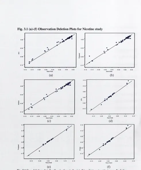
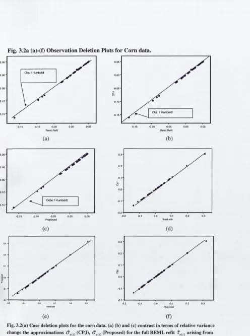
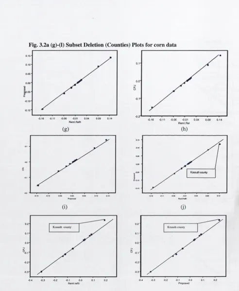
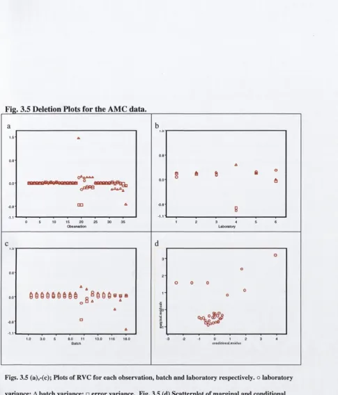
3.1 3.2a 3.2b 3.3 3.4 3.5 3.6(a)-(b) 3.6(c)-(d) 3.7 3.8(a)-(b) 3.8(c)-(d) 3.8(e)-(f) 3.8(g)-(h)Chapter 4
4.1 4.2 4.3 4.3.1 4.4 4.5 4.6 4.7Deletion plots for nicotine study Deletion plots for corn data Deletion plots for soybeans data Plot o f rats’ weight over time Deletion plots for rats data Deletion plots for the AMC data
Log(Cov(e(„,,e,^)) )and Log( Cov(e^,e^^^)) for each observation
\x^
V'“'x I
Plots of ' —^ f o r each subset (rat)
Plot o f modified rats dataset
Log( ) )and Log( Cov{e^, )) for each observation Plots o f the differences between Cov{e^^^,e^^^) and Cov{e^,e^^^^)
I 1 / “ ' Y I
Plots o f J-i--- r-^for each rat.
Page Number
60Plot o f the variance o f the error against
Longitudinal plot of simulated data
p . .
Plot o f —^ - 1 using REM L and proposed method
P
Plot o f ice cream consumption against temperature Deletion plots for ice cream data
D eletion plots for autocorrelation parameter for rats data Deletion plots for modified rats dataset
Exam ple 1- Analysis o f simulated data Exam ple 2- Analysis o f simulated data
108
110
1 1 1 112 113 114 115 116 116
120
121123
124 Singleton deletion scatterplots o f versus for rats data
Subset (rat) deletion scatterplots of versus for rats data
Plots of Cook’s Distance for each rat Singleton deletion plots for corn data Singleton deletion plots for soybeans data Subset (counties) deletion plots for corn data Subset (counties) deletion plots for soybeans data
Plot of Cook’s Distance for each observation for the corn data Plot o f Cook’s Distance for each county for the corn data Scatterplots o f versus for rats data
Scatterplots of versus for corn and soybeans data p Tayl
Plots o f leverage versus --- 1 for the rats data ^((</»
List of Tables
Chapter 3
Page Number
3.1 R V C using the full R E M L refit and the three approaches 61 3.2 Survey and Satellite D ata for C orn and Soybeans in 12 Iow a C ounties 63
3.3 A nalytical C hem istry D ata 73
Chapter 1
Introduction
1.0
Introduction
M odel criticism for the linear m odel (LM ) is the concern o f this chapter. T h e focus o f the thesis is on diagnostics for the linear m ixed m odel (LM M ), w hich is an im portant subset o f the LM fam ily o f m odels. T he m ain diagnostic approaches in the literature stem from consideration o f the LM . T he LM is introduced in this chapter and its m ain variants considered.
C onstructing appropriate m odels for various types o f data is an integral elem ent of m odern statistical analysis. T h e statistical m odel building process is well docum ented in the literature. T he need to assess a m odel’s validity and suitability is an integral elem ent o f this process. T here is a substantial literature on model criticism and diagnostic
m ethodologies for statistical m odels. The principal diagnostic approaches are introduced and considered in this chapter.
1.1 Diagnostic analyses and the statistical modeling process
A diagnostic analysis is a key elem ent o f statistical m odeling. T he structured statistical m odel-building strategy espoused so well by Box and Jenkins (1976) consists o f three m ain steps, m odel identification, m odel estim ation and m odel validation.
At the m odel identification stage, m odels are selected that m ay be appropriate for the dataset o f interest. T he m odel will inevitably involve one or m ore param eters w hose values m ust be estim ated from the data. M odel estim ation consists o f finding the best possible estim ates o f those unknow n param eters w ithin a given m odel. T he final step in the m odel building process is concerned w ith analysing the quality o f the model that we have specified and estim ated. T his involves considering how w ell the m odel fits the data and how the data influences the m odel identification and estim ation processes. T his step is critical to the success o f the m odeling process. If no inadequacies are found, the m odeling m ay be assum ed to be com plete. O therw ise another m odel is chosen in light o f the inadequacies and the process is repeated until an acceptable m odel is found.
M odel diagnostics are prim arily concerned w ith tw o interrelated questions. Firstly, diagnostics are concerned w ith checking how well the fitted m odel resem bles the
observed data. M odel validation approaches focus on residual analysis (W eisberg, 1985). The second elem ent o f m odel criticism is influence analysis. Influence diagnostics are used to analyse the effect o f perturbing the m odel form ulation or data. It is essential that the data analyst identify influential observations that affect the m ajor statistical inference o f the study.
impact on the calculated values o f various estimates than is the case for most o f the other observations”. Influential data can arise due to a mis-specified model or due to
anomalous data. However, influential data may arise within a correctly specified model with satisfactory data. Their presence simply indicates the need for further analysis.
Numerous books and articles consider residual and influence analysis. These include the seminal papers of Cook (1977,1986), Pregibon (1981) and Chatterjee and Hadi (1986) and the books by Belsley et al, (1980), Chatterjee and Hadi (1988) and Cook and W eisberg (1982). These focus on diagnostic methodologies in the context o f the LM with constant variance and independent errors. They have been developed further for application to more general forms o f the LM. In section 1.3 the principal diagnostic approaches for the LM from the literature are considered. Firstly, the LM and its main variants are introduced in section 1.2 below.
1.2
The Linear Model
The defining characteristic o f the LM is that the model is linear in the parameters. McCulloch and Searle (2001) outline a general form of the linear model that may be adapted to describe its main variants. Let y be an N \ 1 vector with N data values and mean ju. V is defined as the variance covariance matrix of Y so
The variant o f the linear model can be defined by specifying jU and V appropriate to the nature of the data being studied. For example, the forms o f // and V for the LM with constant variance and independent errors are
( LI )
where is a p \ \ vector of unknown fixed parameters and X is a Icnown x p matrix and
V = (7^I (1.3)
with / being the identity matrix of size N \ N . The principal diagnostic approaches were developed in the context o f this model with the data deemed to have come from a normal distribution. The General Linear Model (GLM) with normal errors is defined as
Y ~ N { X J 3 , V ) (1.4)
This incorporates many variants o f the LM principal among these being the LMM. The LMM is an important member o f the LM family, which while assuming normally distributed errors permits heterogeneity o f variance. The LMM is a LM where some of the parameters are treated not as constants but as realisations of random variables. The LMM is defined as
Y = X/ 3 + Z y + £ (1.5)
where X and Z s ( Z p Z j, Z^) are known matrices, y^is a vector of fixed effects and 7 is a vector o f random effects with E ( / ) =0, Cov ( y ) = D and (C o v {y , e) ) = 0 . V will then be o f the form Z DZ ^ + A where Z^ denotes the transpose of Z and A = V a r ( e ) . The LM M is considered in more detail in chapter 2.
m odels, p ro b it and logit m odels could be generalised to unify an entire collection o f m odels. T h e generalised linear m odel has been extended to incorporate generalised linear m ixed m odels. G eneralised linear m odels are o f the form
£ ( y ) = / / (1.6)
and
g{M) = ^ P (1-7)
w here g (.) is a know n function called the link function. For generalised linear m odels Y is assum ed to follow a distribution from the exponential fam ily o f distributions. For O rdinary L east Squares (O LS) lin ear regression or for the GLM the hnk function is the identity. T here is an extensive literature on generalised linear m odels with M cC uilagh and N elder (1989) and M cC ulloch and Searle (2001) being the principal texts in the area. In this thesis the focus is on diagnostics fo r the LM M with normal errors and so
generalised linear m odels are not considered in detail.
1.3
M odel Criticism for the LM.
Cook's seminal work (Cook, 1977) in the context of the linear model with constant variance and uncorrelated errors has spawned an entire literature on residuals and influence. The key to this developm ent was Cook's dem onstration that the effects on estimates p o i (3 o f deleting each observation in turn could be cheaply computed as a by-product o f the fitting procedure. The impact o f the deletion o f each observation can be computed en bloc. This ease o f computation has led to these deletion diagnostics becoming a feature of statistical software for this OLS situation.
Various papers have been written generalising these diagnostic measures to the GLM with the variance covariance matrix defined as crV . These papers include Martin (1992), Haslett and Hayes (1998), Haslett (1999) and Baade and Pettitt (2000). The formulae derived to com pute the diagnostics are based on the key assumption that V is unchanged when observations are deleted. The effect o f this assumption on the accuracy of the various diagnostic measures has not been explored in detail in the literature. This issue is considered in chapter 5. The various diagnostic approaches from the literature for the GLM with a single com ponent o f variance are outlined below.
1.3.1 Residual Analysis
The com putation and analysis of residuals are key elements of any diagnostic analysis. The classic or marginal residuals are calculated by subtracting the estimate o f the expected value o f Y , E( Y) = X P from the observed Y with = { X ^ V ' X y ^ X ^ V ' ^ Y . The marginal residuals are thus defined as
If w e define Q = V ' - / / w here / / = y " 'A :5 a n d B = { X W - ' X y ' t h e n it can be easily show n that e = V QY and thus V a r(e ) = V QV . The m arginal residuals are b y products o f the fitting process and are easily calculated. For the case o f OLS linear regression, graphical plots o f the residuals are used to validate m odel assum ptions.
H ow ever, for the G LM the m arginal residuals are not independent even asym ptotically (unless V is diagonal). O ne general approach has been to rotate the residuals by
(var(e)y ''^ w hen ordinary least squares applies. Theil (1965) provides an exam ple o f this approach. The principal disadvantage o f diagnostics based on this approach is the
difficulty in interpreting them .
W hile the m arginal residuals based on the best linear unbiased estim ator (BLU E) o f Y for the G LM are well defined, residuals based on the best linear unbiased predictor (B L U P) o f Y are degenerate. This is the case because the B L U P o f an observed datum y. given the observed data Y is y . . T his has led to the study of conditional residuals referred to by som e authors as deletion prediction residuals. Let Y^ be partitioned as { Y / , Y j } so that
y is a stacked vector. T he conditional residual or deletion prediction residual has been defined (M artin, 1992) as the difference betw een Y^ and 7^ (7^) the B L U P o f Y^ given Y^ and given an estim ate o f (V ) the m atrix V . Therefore Y^(Y^) is an approxim ation as we still use V rather than . For notational convenience V is referred to as V . T hus the conditional or deletion prediction residual can be defined as
f,., = n - (X . A n )
+
( n
(
1
.9)
e = A V 'e,
■( •)(1.10)
w here a vector containing the le a v e -1-out conditional residuals and A = l /d i a g ( 2 ) .
T his result is extended to subset deletion for arbitrary subsets in H aslett and H ayes (1998) and M artin (1992) with - Q a a ~ ' ■ H aslett (1999) and H aslett and D illane (2004) highlight the im portance o f the conditional residual in the com putation o f the
various deletion diagnostics. They show that m any o f these statistics are sim ple functions
M artin (1992) proposes alternative conditional residuals called “prediction residuals” . T hese are defined as
T hese two types o f conditional residual depend on w hich estim ate o f P is used in their calculation. A n estim ate o f P based on all the data produces w hat M artin (1992) term s a prediction residual. T he deletion prediction residuals are based on [5 estim ated from .
H ow ever, they are som ew hat counter intuitive as the estim ate o f P used in their com putation is based on all the data.
T he third categ o ry o f residuals considered is recursive residuals. R ecursive residuals w hich arise prin cip ally in the tim e series literature given the tim e ordered nature o f such
o f e.
B oth m easures are com puted using V and are thus approxim ations. M artin’s ‘prediction’ residuals are related to the m arginal residuals by
data are applicable to some LMM applications. They are directly connected to the conditional residuals. The recursive residuals f, are a contrast between Y, and an estimate of in which the unknown parameter ( i is estimated from
= {Y /,s < t ) . Haslett and Haslett (2005) show that r, = V~' ' ^X{f t {Y) ~ ft{Y^,))
-B with -^(>r) the conditional residual for the subset (s = . The past
values on which the prediction of F, is based are clearly defined for tim e series data.
However, the use of recursive residuals in other areas has produced quite imaginative definition o f the "past". Pickford and H aslett (1999) order data by measure of size and consider both a "backward" and "forward" interpretation in computing the recursive residuals. A review by Kianaford and Swallow (1996) point out that the recursive residuals are not unique as the data can be ordered in any number of ways and are thus problematic.
1.3.2 Contributions to the lack o f fit statistic
The lack-of-fit statistic is defined as S ( Y ) = eW^'e = Y^ QY . It is central to the analysis of the linear model reflecting the distance o f the data from the best fitting linear model. By using appropriate decompositions o f 5 (7 ) or for simplicity S the im pact of individual observations or groups o f observations may be assessed. Using the earlier result
e - A V ~ ' e S may be rewritten as
S = e 'A -‘S = X g „ e ,e ,„ ^ ± C , (1.13) /= ! /= !
Thus C ,, the contribution to the lack-of-fit statistic can be written as a weighted sum o f
w hat these two types o f residuals are m easuring. A m arginal residual m easures the
difference betw een the data and the underlying trend o f the m odel, a global feature that
has a certain structural perm anence throughout all values o f the design m atrix X . T he conditional residuals are m easures o f the difference betw een the data and the expected
value o f the data ‘given the re st’. Thus the conditional residual can be view ed as a
m easure o f the local aspects o f the fit. H aslett and H ayes (1998) use plots o f e. versus to explore both aspects o f the m odel fit.
1.3.3 Deletion Diagnostics for Influence Analysis
D eletion diagnostics are established tools for influence analysis. As C hatterjee and Hadi
(1986) observe “a bew ilderingly large num ber o f deletion diagnostic m easures have been
proposed for the O LS regression m odel” . M artin (1992) and H aslett and H ayes (1998)
provide derivations o f these diagnostics for the G LM . T hese derivations rely heavily on
detailed identities associated w ith the inverses o f partitioned m atrices. H aslett (1999)
outlined the “delete = replace” approach which provided a general sim ple and intuitive
derivation o f deletion diagnostics. Intuitively, it m ay be stated thus: there is an
equivalence betw een (a) the reduction o f a m odel by the deletion o f a subset o f
observations and (b) the replacem ent o f the subset by its B L U P given the rem aining
observations. Its value is that the reduced m odel m ay be analysed in term s o f vectors and
m atrices o f the original dim ensions, considerably sim plifying com parisons with the
original fit.
T he principal m ean structure diagnostics are D F BETA and C o o k ’s D istance. The “delete= rep lace” approach is described in the context o f deriving D F BETA . W e form
Y- = (F „ (r,), y j . H aslettt (1999) show s that p { Y ,) = . DFBETA^ is defined as
provides a very simple derivation of the DFBETA^ statistic for the GLM case. The
“delete = replace” approach is exploited in chapters 3 and 4 for developing covariance structure diagnostics.
The DFBETA^ statistic is a measure o f the impact on the mean parameter estimates o f deleting an arbitrary subset of observations a . An extension o f DFBETA^ is its
standardised form DFBETAS^ which is the DFBETA^ statistic standardised with respect to the standard errors of the components of ^ { Y ) = a ^ { X ^ V ~ ^ X y ' . A large value of
DFBETAS^ indicates that the subset a has a sizeable impact on the regression
coefficient. As a result, the analyst must observe N \ p statistics in assessing influence
on the mean param eter estimates.
In addition, associated with each data point or subset of data points is a single essentially a composite measure of the influence on the set of coefficients. This quantity or statistic is Cook’s Distance, and is defined as
D F B E T A j(X ^ V -'X )D F B E T A ^ / p a " (1.14)
Cook's Distance is a measure, representing the standardised distance between the vector of estimated coefficients and A large value for Cook's Distance implies that the
subset a exerts undue influence on the set of coefficients. To determine which specific coefficients are affected one must direct attention to the DFBETAS^ statistics. M artin
(1992) describes some variants of Cook’s Distance due to different standardisations. These include a l , { X ^ V - ' x y and •
= Y ^ Q Y l { N - p) with 0^1^)- ~ w here o denotes the num ber o f
observations in subset a . It can be easily shown that
y^QY-ylQa»='^ia"QaaK^
d ' ' 5)
T his >s the M ahalanobis distance o f y^from . It is easy to show
that
N - p - o
It is thus easy to ‘studentize’ externally with variances based on as for the tw o
variants o f C o o k ’s D istance above. A n influence m easure based on the above form ula is
the R elative V ariance C hange (R V C ) w hich is defined as
w hich from above equals
(1.18)
N - p - o
O utlying values in the Y space will have a large effect on the residual sum o f squares.
A num ber o f m easures based on the im pact o f deletion on confidence ellipsoids have
been proposed. T hese include the C ovariance R atio (CVR) and the A ndrew s Pregibon (AP) Statistic.
The C ovariance R atio is defined in equation 1.19 below
C V R , ^ ( a )
y a a
| s “ ( x ' ' v ' x r ' | V / Q a a
(1.19)
w here = (V^^) '. This statistic has no standard error type scaling (B elsley et al,
1980). H ow ever, it is clear that a value exceeding 1 implies that the subset deleted provides an im provem ent i.e. a reduction in the estim ated generalised variance o f the coefficient over w hat w ould be produced w ithout the subset o f data. A sim ilar statistic in the literature is the A P statistic w hich is proportional to the reciprocal o f the CV R.
_
( N - p - o ) a ( ^ ) Q o a ( n - p ) a ^ (X"^V-'X)| ( N - p ) a ^ y a aA s we observed w hen considering the R V C the deletion o f an observation which is outlying in the Y space will result in a m arked reduction in the residual sum o f squares (R SS) o r a large difference betw een { N ~ p)&^ and ( n - p - o ) a f ^ y An observation w hich is outlying in the X and V senses will m anifest itself in the change in
Thus the A P statistic is designed to detect observations influential in both th e X ,V and
1.3.4 Subsets and Singletons
The various diagnostic measures outlined above are attractive because o f their ease o f
computation for singleton deletion. The entire set o f singleton deletions may be
computed en bloc. In this section we consider subsets involving more that a single
observation. Consider a partition P of the indices o f Y into blocks aj , j = \ , , k . It is
more challenging to compute when k ^ N , where the subsets are not all singletons.
However, the conditional residuals and results in A ppendix 1 allow computation o f some
o f these diagnostic measures en bloc. Let D^-Var{e^^^) = ' • It can be easily shown
that = D pQ Y where Dp is block diagonal with blocks , j = 1, k . The entire set
of conditional residuals gj^^may also be computed from the following important
interrelationships.
D p - 'e p = ^ - 'e ^ ,^ = V - 'e (1.2 1)
The DFBETA^ statistic can be computed from DFBETA^ = B . The p x A: matrix [ o j
DFBETAp m ay be com puted from DFBETAp = B E where £ is an N \ k matrix with the
77/2 colum n o f £ containing and 0 . DFBETA^ will be a /? x A: matrix with the jr/z
column containing DFBETA^ . An alternative expression from equation 1.14 for C o o k ’s
Distance is given in equation 1.22 below
C o o k ’s Distance ( 1,2 2 )
p d
C o o k ’s D istance p = e^p^GE! p a ^ (1.23)
w here G is block diagonal w ith elem ents and where H = V . An alternative
approach to com pute C o o k ’s D istance p , which doesn’t involve form ing the m atrix E is also available. Let the op erato r □ ^ be defined such that for any two vectors / , g o f dim ension N and a partition P , / □ ^ ^ is a row vector o f length k w hose elem ents are
S ,g ^ /g ,( H a s le tt and H aslett, 2005). Using this notation C ook’s D istance ^ m a y b e
com puted as GU p e^p^ / .
The issue o f external studentisation w as considered in section 1.3.3. and the need for an Y ^ O Y - e ^ 0 e updating form ula for (7,^^, highlighted. This was defined as =--- —— .
N - p - o T he com putation o f <7,^^ is quite straightforw ard. Let 5 denote the k x 1 matrix with elem ents Y ^ Q Y and 5(p)the k x 1 m atrix with elem ents Y^Q^^^Y^. S^p^ is com puted from S- e^p^D~' Q pS^py T h u s d ^p^ -S^ p^l s where ^ is a A: x 1 m atrix with elem ents
N - p - O j . The RVC^p^ is easily com puted using these results. It was not possible to develop m ethods to com pute the A P and CVR statistics easily en bloc as both statistics involve com puting the determ inants o f various matrices.
1.3.5 Leverage
In the O LS case leverage can be adequately described in term s of the rem oteness o f an observation in the X space (C hatterjee and Hadi, 1988, pg 95). High leverage cases are identified through the diagonal elem ents o f the H matrix w here H is defined as
X ( X ^ X ) “'X ^ a n d X is full rank. If / / is of full rank then t r { H ) = p . T h e average siz e o f a diagonal elem ent is p i n . T he values 2 p l n and 3 p ! n are used as benchm arks
statistic is analogous to W ilk’s statistic (Cook and W eisberg, 1982, pg 129) which is used
to detect a single outlier in multivariate data.
D raper and John (1981) advocate this statistic as a generalized measure of leverage that
could be used for both subset and singleton deletion. High leverage subsets are identified
by small values of this measure. However, they also point out that high leverage cases
identified from this measure need not correspond to those identified from H .
In the GLM context the issue of leverage becomes more complex. Schull and Dunne
(1988) and consider transforming the data to the OLS situation with K Y = K X (3+ K e
and Var ( Ke ) = where K is such that K = V " '. The associated H matrix will be
K X { X ^ V ~ ' X y ' X ^ . Schull and Dunne (1988) use the eigenvalue and eigenvector
decom position of V to obtain K whilst Puterman (1988) takes K as lower triangular.
However, other K are possible with examples considered in the context of the LMM in
section 2.3.3. M artin (1992) shows that the most fundamental quantity, which might be
considered the generalization of leverage to dependent data for observations is q-- the
diagonal elem ents o f Q. An observation dem onstrating high leverage will have a small
causing 1 / q.. to be large. The q.. may be scaled by dividing by the corresponding
diagonal elem ent o f V“’ .
The issue o f high leverage subsets with o > I receives little attention in the literature for
either the case when V - 1 or for the GLM situations. However, a recent paper by
Dem idenko and Stukel (2005) outline an approach for identifying high leverage subsets
in the context o f the LMM. This is considered in chapter 2. The approach may also be
^ m atrfx associatcd with subsct a. Then
k
^ t r { H ^ ) - p and thus the average value o f the tr{H^ ) = p i k . They propose tr{H^ ) 7=1
as a leverage m easure. A larger than average value o f t r( H^ ) points to an influential
subset j .
T he statistic defined in equation 1.2.4 is easily applied to the GLM situation. U sing the
transform ation to O L S w ith X* = V~' ^^X the corresponding expression for the G L M in
equation 1.25 is easily derived.
yT I / - I Y
I (1.25)
A gain as for the O L S case high leverage cases identified from this m easure need not
correspond to those identified from the other m ethods outlined above.
1.3.6 Local Influence and the Influence Graph
C ook (1986) developed a general m ethod for assessing the local influence o f minor
perturbations o f a statistical m odel. For a given set o f data let L( 0 ) denote the log
likelihood corresponding to the model w here 0 is a vector o f unknow n param eters.
Perturbations are represented by a m atrix co. The likelihood displacem ent is defined as
LD{co) = 2 [ L { Q ) - L { Q J ] (1.26)
The ‘influence g rap h ’ o f LD{co) versus as varies in Q , the range o f possible
perturbations, show s the sensitivity o f variables to perturbation. This technique m ay b e
used to assess the im pact o f perturbing the data, the param eters or individual covariates.
1.3.7 Inflnitesimal Influence
Pregibon (1981) introduced the concept of infinitesimal (infinitely small) influence in which the sensitivity o f a statistic to a small perturbation o f data or model may be
considered. As the focus is on infinitesimal change, the derivative is the natural measure of influence. The infinitesimal influence o f the ith observation v, on some function of
Y dented as F{Y) is defined as
(1.27) d ( y . )
The influence analysis based on the derivative in equation 1.27 is referred to as
infinitesimal data influence analysis. The partial derivative is evaluated at the current data so no re-estimation is needed.
This approach also allows consideration of small perturbations in the model or model influence. Let l{6) be the log-likelihood o f the postulated model. This model is nested in a more general or “parent” model that is dependent on an additional param eter <y. Let
t{co) be any statistic or characteristic of interest as a function o f co, e.g., the Maximum Likelihood Estimate (M LE) which maximizes the log-likelihood 1(0/ co). Demidenko (2004) defines the influence of t with respect to a possible departure from the postulated model as
This approach is similar to Cook’s local influence approach outlined above. The
difference between the approaches is that Cook (1986) took the likelihood as the measure
of model departure. This approach expresses model departure in terms of the
characteristic o f interest t . Obviously if t is taken as the likelihood displacement both
approaches are identical.
The infinitesimal approach is attractive as it is a general tool and can be applied to any
statistic to assess the influence o f data or model perturbation. It is also easy to compute
as the analysis is based on the current estimate and does not require additional
computations. It also has the advantage that it does not require a distribution assumption.
1.3.8 Fixed effects joint and conditional influence
There are situations when an observation is not influential individually but taken in a
group with other observation may be highly influential. On the other hand an individual
observation may be influential on its own but when taken with another observation it may
have little influence. These effects are described as “swamping “ and “masking” in the
literature. In the time series literature it is referred to as “smearing” though the correlated
nature of the data worsens the problem. Successive deletions have been used (Lawrence,
1995), (Baade and Pettitt, 2000) to identify conditional influence in the fixed effects.
Haslett (1999) has used the “delete=replace” approach to derive conditional deletion
diagnostics. Interest focuses on the deletion o f Y. given that Y. has already been deleted.
The results extend from partitioning Yas {Y^,Yf^,Y^) which may also be written as
(^ab^c) with = p{Y^) and - Y^, {Y^). is then contrasted with
and this is a measure of the effect on ^ o f deleting Y^ given that Y^ had already been
Afc)
P { a h ) ~ ^ P P ( a h ) ) P ( h ) ' ) - ^ \ a h ^ ( a h ) ^ \ h ] ^ ( b ) ~ ^ [ a h ] ^ (a\h) (1.29)
where denotes the columns o f corresponding to F^and toY^ and defined as
^<ah) ~ (Ofl ’ ^(fc) )• The conditional C ook’s Distance is defined as
where refers to the block of H associated with the [ab] rows and columns. The
conditional deletion o f subsets and their impact on the variance param eter d ^ c a n be also
be derived. 5 ( 7 ,,) = S ( Y ^ , ^ ) - = S ( Y ) - S ( Y ^ , , ) - S { Y ) - S(Y^^,,). Therefore
where m is the size o f subset { a b ) .
1.4
Conclusions
Model criticism is an essential elem ent o f the model building process. There is an
extensive literature on diagnostic measures for the LM. These diagnostics help the data
analyst to test model assumptions and identify outlying and influential observations. The
methodologies fall into two broad categories, residual analysis and influence diagnostic
techniques.
There is a substantial literature on the use o f residuals for checking model assumptions
and exploring model fit for the simple linear model with Var{Y) / . However, for the
GLM the literature is sparse. McCulloch and Searle (2001) contains no reference to
residuals or model checking. Christensen (1987) devotes a chapter (Ch 13) to residuals.
D = p ^ H p
a\h [ah.ab] (a\b) (1.30)
H ow ever, it focuses on the sim ple case o f Var{Y) I only. W hittaker (1990) in
considering graphical m odels for m ultivariate data and Cox and W erm uth (1998) also in the m ultivariate context m ention residuals only in the OLS setting.
A large num ber o f deletion diagnostic m easures have been proposed to study influential observations in OLS linear regression analysis. M any o f these m easures have been extended to the G LM and are sum m arised by M artin (1992) and H aslett and H ayes (1998). T hese extensions are based on the assum ption that the covariance m atrix V is unchanged follow ing deletion. T he assum ption allow s the various m easures to be easily derived. H ow ever, the im pact o f this assum ption on the accuracy o f the diagnostics is not clear from the literature.
T he extent to w hich the various diagnostic m ethodologies proposed in the literature may be applied to the LM fam ily o f m odels varies. The focus o f this thesis is deletion
Chapter 2
Diagnostics for the LMM
2.0
Introduction
This chapter focuses on the LM M . T he m odel is an im portant m em ber o f the LM fam ily
and the focus o f this thesis is on deletion diagnostics for the LM M . In chapter one, the
various diagnostic m ethodologies and m easures w ere outlined in the context o f the G LM
with a single com ponent o f variance. T h e LM M m ay have more than one com ponent o f
variance, w hich m akes a diagnostic analysis m ore com plex for this m odel. In this
chapter, the diagnostics are review ed in the context o f the LM M .
D iagnostic analyses arise at two stages in the LM M . T hese are at the estim ation o f the
covariance structure param eters and at the subsequent estim ation o f the m ean structure
param eters. M ean and covariance structure diagnostics for the m odel from the current
literature are review ed and the need for such m ethods highlighted. Inadequacies and
shortcom ings in the diagnostics proposed to date in the literature are clearly enunciated
and the issues arising from this chapter act as the m otivation for w ork in the follow ing
2.1
The Linear Mixed Model
LM M s appear under a variety o f titles in diverse literatures. In sociological research,
they are often referred to as m ultilevel linear m ode (M ason et al, 1983). Lindley and
Sm ith (1972) introduced the term hierarchical linear m odels. This was adopted later by
Bryk and R audenbush (1992) and by m any others since. In the biom etrics literature the
term s m ixed effects m odels and random -effects m odels are com m on. Exam ples include
Laird and W are (1982) and D iggle (1990). They are also referred to as random -
coefficient regression m odels in the econom etrics literature while in som e statistical
literature they are referred to as covariance com ponent m odels (D em pster et al, 1981),
(L ongford, 1987). T he m any areas o f application o f this m odel suggest that sim ply
com putable diagnostics w ould have wide appeal.
D evelopm ents in num erical approaches to covariance com ponent estim ation allied with
advances in statistical softw are have allow ed mixed and random -effects m odels to be
applied extensively. L ongitudinal studies are an active area o f application for the LM M .
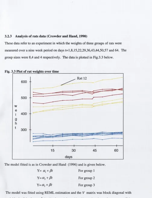
H and and C row der (1996), Lindsey (1993) and Diggle et al (1994) all contain chapters
describing the application o f LM M s in the analysis o f longitudinal data. In such studies a
response is m easured repeatedly over tim e on a num ber o f experim ental units or subjects.
T he focus o f any diagnostic analysis for these studies is likely to centre on the
experim ental units as well as on the individual observations.
It is clear that any proposed diagnostics m ust be easily com putable for both observation
and subset (other than singleton) deletion, as a thorough diagnostic analysis should
involve both. In the context o f longitudinal data, O uw ens (2001) dem onstrates the
necessity to use observation influence m easures in addition to subject based influence
m easures as existing subject influence m easures may fail to detect influential subjects d u e
The LMM was defined in 1.5. with the variance covariance matrix V = ZDZ^ + A
r
where A = Var{e). An alternative expression for V = A + ' ^ a f Z . Z ^ ^ with cr,^ denoting i = \
the variance of the random parameters y. and Z- is a design matrix relating y. to Y .
Models for A = Var(e) describe the auto-covariance structure in the data. The matrix
A is often of the form . However, when there is autocorrelation in the data A will
include a correlation param eter p . This is common in time series and longitudinal data.
Various models for A have been proposed in the literature. Hand and Crowder (1996,
chapter 6) and Diggle Liang and Zeger (1994, chapter 5) outline the principal parametric
models for the auto-covariance structure.
There are two stages in the fitting of such models; these may be carried out
simultaneously or sequentially. The first is the modelling and estimation of the
covariance structure V. The second stage in fitting such models involves the estimation
of the fixed param eters P . The estimation of these involves the use o f the BLUE o f P
which is well known from the classical theory to be . The
standard estimation methods used at both stages of the fitting process are sensitive to
unusual observations. Therefore any diagnostic analysis needs to be conducted at both
stages for LM M s.
The w ide usage o f the LMM as reflected in the literature indicates it is likely that easily
com putable diagnostics for the model (the focus of this thesis) would be appealing and
have w ide usage. In this thesis diagnostics for both stages in the fitting process are
considered. In chapter 3 cheaply computable diagnostics for the variance components are
proposed. C hapter 4 develops approaches for assessing the influence of observations on
used to model the autocovariance structure in data. These methods are also applicable for
the important com pound symmetry case. The focus in Chapter 5 is on mean structure
diagnostics for the LMM. The methods developed in the thesis exploit elements of the
various model fitting and criticism procedures in the literature and are considered in
sections 2.2 and 2.3 respectively.
2.2
Methods of estimation
Estimation methods for the LMM are detailed in many books and papers, the principal
approaches being ANOVA, maximum likelihood (ML), restricted maximum likelihood
(REM L) and minimum norm quadratic unbiased estimation (MINQUE). ANOVA and
REM L methods are used in chapters 3 and 4 to develop diagnostic methods for the
variance and correlation param eters in LMMs. This consideration of estimation methods
is confined to these approaches.
2.2.1 ANOVA m ethods and H enderson’s Method III
Various ANOVA approaches have been developed to estimate variance components for
random and mixed models. For balanced designs, they produce unique, computationally
inexpensive and intuitive estimates. Indeed for the balanced case the solutions to the
REM L equations are identical to ANOVA estimators (Searle et a i, 1992). However, for
unbalanced data there is no unique set o f sums of squares that can be used. Early
extensions of ANOVA methods to unbalanced data focused on the 1-way classification.
These included work by Cochran (1939) and W insor and Clarke (1940).
Henderson (1953) extended the approach to higher order classifications motivated by his
interest in estimating variance components in a genetics setting where available data can
be voluminous but severely unbalanced. The approaches outlined in this paper Decame
models unlike the other methods, which are restricted to the class of models that they
may be applied to. M ethod I is applicable only to random models w hile Method II
cannot be used if there are interactions between the fixed and random effects. The
motivation for outlining Method III below stems from its usage in section 3.1.1 to
develop diagnostics for the variance com ponents in the LMM
In the formulation of the LMM in equation 1.5 there was a clear distinction between the
fixed and random effects. In considering Method III the fixed effects p and random
effects y are combined into a single vector rj and the model may be re-expressed as
Y = M^ j j + e with consisting o f ( X .Z ^ Z j , Z^) and having dim ension N \
i p + q) . Similarly consists of ( X ,Z p Z2, Let
Q, = l - M^ { M J M M J . The variance com ponents may be estim ated from taking
expected values of the differences in the “sums o f squares” = Y^Q^Y . To estimate cr^
we consider the expected value o f the difference between and
It can be easily shown that Q^_^X and Q^X =0 and therefore {Q^_^ - Q ^ ) X = Q
r
Re-expressing V as a l + ^ a f Z . Z ^ ^ we can express {Q^_^ - Q ^ ) V as
(2 . 1)
because (g^_,
- Q ^ ) Z . Z j
= O fo r i = 1,.../ - - I . Given these results-
tr[{Q^_,
-a)<^0 +(a-i
=
- a ) ]+
< y > m r - ^ - Q r (2.2)E { S ^ ) = t r { Q y ) = a l t r[Q ^ ]
An unbiased estim ate o f a l is thus &l = S J t r ( Q ^ )
An unbiased estim ate o f is
= [
5
,., - s , -a„^rr(a-,
-Qr)zx ]
(2.3)
In a sim ilar fashion we can estim ate by taking expectations o f sum s o f squares based
on and M w hich gives
E [ Y ^ (a_2 - Qr-x = tr[{Q,-2 - Qr-> ) y ]
= tr[{Q,_2 - Qr-x )c^o + (2 .-2 - e .- i v , l , + (a _ 2 - a - ,
An unbiased estim ate cr^\, is thus
[ 5^. 2- 5. . , - c T o ' ^ K a - 2 - a - . ) - ^ ^ ' f K ( a - 2 - a - , ) z . z / ) ] / M ( a - 2 (
2
.
4
)
T he rem aining variance param eters c r f , a l , ^ can be estim ated in a sim ilar fashion.
T his approach is developed in section 3.1.1 to provide estim ates o f the change in the
variance com ponents follow ing subset deletion.
2.2.2 REML Estimation
T he other estim ation p rocedure exploited in chapter 3 is REM L. T he R E M L method w as
introduced by Patterson and T hom pson (1971) as a way o f estim ating variance
com ponents for the G L M . T he im petus for this approach to param eter estim ation, in this
case arises from the inability o f standard M L estim ation to produce unbiased es:imates.
T his is well know n in the case o f the LM with independent errors. T he maximvm
likelihood estim ate o f <j^ is R S S / N w here N is the num ber o f data values. THs is a
biased estim ate o f w hereas the R E M L estim ator o f is the unbiased estirrator
<T^ = R S S /N - p . T hus R E M L estim ation gives an unbiased estim ate fo r <j^. I; can b e
the distribution o f F ’does not depend on . One approach to achieve this is by taking A
to be the matrix which converts Y to ordinary least square residuals A = 1 - { X ^ X ) ~ ' .
Then Y* has a multivariate normal distribution with mean zero w hatever the value of J3.
Any full rank matrix with the property E[F*] = 0 for all P will give the same answer.
The equations for solving iteratively the REM L estimates are
X o -;M Z ^ Z /G Z ,Z ,"G ] = Y ^ Q Z Z j Q Y (2.5)
7 = 1
for i = 0 , r and where Q is as defined in section 1.3.1 (Christensen, 1987,pg.237).
REML is routinely used to estimate the variance components in LMMs. Various studies
have considered its merits relative to ML. These may be summarized by Diggle et a l ’s
(1994, pg. 68) observation that in many cases both will give very sim ilar results but when
they do differ substantially REML estimates are preferable.
When com puting deletion diagnostics the data will often be unbalanced after deleting a
subset. There is agreem ent in the literature that for unbalanced data R EM L is preferable
to ANOVA approaches for estimating the variance components. Historically ANOVA
methods were preferred as REM L was impractical because o f its com puting
requirements. However, this is no longer an issue. Nevertheless, A NOVA methods are
likely to continue being used (Searle et al, 1992, pg.l68). This is because many
researchers are com fortable with the closed form ANOVA estimators and find M L or
REML approaches too theoretic and are overawed by the mathematics involved.
Therefore in chapter 3 diagnostic methods based on both ANOVA and REM L are
2.3
Diagnostics for the LMM
As outlined in chapter 1, there are two principal strands to any diagnostic analysis. These
are residual analysis and influence analysis. For LMMs with more than one variance
component, these analyses become more complex. The consideration of these issues is
relatively sparse in the literature. For example, McCulloch and Searle (2001) contains no
reference to diagnostics in the entire text and Christensen (1987) focuses his discussion
exclusively on the LM with independent errors.
2.3.1
Residual analysis for the LMM
The marginal residuals
e
defined in equation 1.8 are estimates of the true model errors£ = Y - X P .
For the LMM these errors may be defined by a number of independentunderlying variables. The estimates o f these underlying variables are termed innovation
residuals (Haslett and Haslett, 2005). In time series the innovations are the white noise
processes that drive the model and the term is drawn from the time series literature. The
marginal residuals for the LMM defined in equation 1.5 incorporate the innovation
residuals with
e = Z y + e .
T h e f are "pure error" and ther
terms haveinterpretations as independent random deviations from an overall mean structure for sub
groups o f the observations
Y .
The innovation residuals are estimated asZ y
ande - Z y
with the random effects parameters estimated
by y = DZ^V^'e
=DZ^QY
(Searleet al,
1992). They are related to the conditional residuals with f The term
‘innovation’ for these residuals is only appropriate if / and
D
is diagonal.Several papers have considered residuals for the LMM defined in equation 1.5 with
P o c /a n d
D
being diagonal. M any distinguish betweene
andZ y .
Lange and Ryan(1989,pg628) and Oman (1995) refer to the
i
as "residuals". Oman (1995) uses the term"model" residuals for the
Z y .
Longford (1993, pg66) calls the£
and t h e f "elementarynatural interpretation o f residuals associated with individual elem ents o f / . Particularly
for longitudinal data, subsets com prising m ultiple observations are referred to as
"subjects" or "cases". W eiss and L azaro (1992) in the context o f longitudinal data
analysis describe a useful exploratory approach for m odel specification and for the
identification o f anom alous data based on plotting these residuals against time.
W aternaux et al (1989) and O m an (1995) use residuals based on the y to check model
assum ptions and identify outlying observations.
T he standardized conditional residual o f equation 1.9 is defined as .
This statistic m ay be externally o r internally studentised. T he denom inators for the
internally and externally studentised versions are and (<7(„j^(2„^)“')'^^
respectively. For the single com ponent o f variance case either version is applicable.
H ow ever, for the LM M w ith m ore than one variance com ponent external studentisation is
problem atic. T here is a need to update each variance com ponent follow ing deletion.
There is no ch eap com putational m ethod for doing this. Externally studentised
conditional residuals are not com putationally feasible in this situation. M ethods for
estim ating the ch an g e in the variance com ponents follow ing deletion are proposed in
chapter 3.
The literature on residual analysis for the LM M is relatively sparse. M cC ulloch and
Searle (2001) contains no reference to residuals or m odel checking. C hristensen (1996)
devotes a ch a p te r (Ch 13) to residuals though it focuses on the sim ple case o f
Var(Y) oc / only. It is cle a r that for the LM M residual analysis is m ore challenging than
for the sim p le O L S case o r indeed for the G LM w ith a single com ponent o f variance.
C urrently resid u al analysis fo r the LM M w ith m ore than a single source o f variation is
2.3.2 Deletion Diagnostics for the LMM
Within the LMM deletion diagnostics are not routinely used despite huge advances in
computing. Diagnostic issues arise at two stages in the LMM. These are (a) the
estimation o f V by some V and (b) the subsequent estimation of the regression
coefficients j5 and y given V . Christensen et al (1992) propose that influence analysis
should begin at the first stage. However, the majority of the research on diagnostics for
the LMM focuses on (b). Hodges (1998) and its discussion reviewed much of this
literature under the heading of the hierarchical model. Atkinson (1998) in the discussion
o f Hodges (1998) remarks on the fact that V is taken as fixed and observes that this is a
weakness in such research. Related work by Tan et al (2001), Ouwens et al (2001),
Bannerjee (1998) and Bannerjee and Frees (1997) all assume V is fixed following
deletion. The impact o f this assumption is explored in section 5.1 of chapter 5. The
various deletion diagnostics outlined in section 1.3.3 are reviewed in the context of the
LMM below.
The principal mean structure diagnostics are DFBETA and Cook’s Distance. These
diagnostics are used to identify data influential on the fixed parameter estimates. In
many studies involving LMMs the random parameters may be the focus of interest. An
analogous diagnostic based on DFBETA for the random parameters DFGAMMA^ is
f - . Haslett and Dillane (2004) show that this may be estimated as
vO y
This may also be standardized with respect to the standard error of
the components o f / = D Z Q Z ^ D . The standardized version would correspond to the
DFBETAS statistic. Using results in section 1.3.4 DFGAMMAp - D ZQE and thus
The most popular influence measure in the regression literature is Cook’ s Distance
(Bannerjee, 1998). However, a number o f authors have demonstrated the limited
effectiveness o f the diagnostic in the L M M context. A general criticism o f Cook’ s
Distance is as a composite measure, an observation with a moderate influence on all
regression coefficients may be judged more influential than one with a large influence on
one coefficient and negligible influence on all others. This has led to the development o f
the idea o f partial influence. Partial influence involves examining the influence on
m dividual parameters or on a given subset o f parameters. Cook and Weisberg (1982)
defined the partial influence o f the \th observation on 0 where 0 = L P that is a linear
combination o f the mean parameters P as
Bannerjee and Frees (1997) and Bannerjee (1998) use the partial influence approach to
explore the impact on subject specific parameters and on the population parameters o f
deletion. Tan et a l (2001) demonstrate that influential observations having a large effect
on the subject specific parameters are not always detected by Cook’ s Distance owing to
large between subject variation. They propose a conditional version o f Cook’ s Distance
by conditioning on the subjects. The statistic is decomposed to measure the impact on
the fixed parameters and on the random parameters. It is defined as
The first term may be interpreted as the impact o f deletion on the fixed effects, the
second term as the impact on the subject specific random parameters and the third term as C, (L) = ( 0 - 0 , , ) " (L" X " V - 'X L ) ( 0 - 0 , , ) (2.6)
c
conda m easure o f the covariation betw een the change in the mean profile and a change in the
position o f the subject specific profiles relative to the mean profile. They rem ark w ithout
supporting analysis that the third elem ent can be neglected. This approach is also based
on the assum ption that V is unchanged follow ing deletion.
T he RV C defined in equation 1.17 is one o f the few diagnostics that can be easily
applied to the m ultiple variance com ponent LM M case. Longford (1993) observes that
the RV C is applicable for the LM M as a m eans o f assessing the im pact o f deletion on
each o f the variance param eters <Tq , .... It is used for this purpose in chapter 3
T he C V R and A P statistic are significantly m ore difficult to com pute for the LM M w ith
m ultiple variance com ponents. T he issue is sim ilar to that encountered with external
studentisation. T he C V R sim plifies for the single com ponent o f variance case as outlined
in equation 1.19. T here is no easily com putable accurate estim ate o f unless it is
re-estim ated. I f the re-estim ate is to be accurate each o f the variance com ponents needs to be
updated.
2.3.3 Leverage
F or the LM M both the covariates and the random effects m ay influence the leverage
m easure. D em idenko and Stukel (2005) propose a m ethodology for considering leverage
in the LM M . T hey p ropose a leverage m easure com prising two com ponents; one
m easures high leverage data in the X space and the other in the Z space. They co n sid er
leverage as the partial d erivative o f the predicted value with respect to the corresponding
dependent variable. F or the LM M Y = X P + Z / i s the predicted outcom e conditional on
/ j y
the estim ated random effects / w i t h // = X ( X ' V ^ ' X ) ~ ‘X' V~' + Z D Z ^ Q = H^ + / / j .
h ig h lev erag e o b se rv a tio n s in e ith e r the X or Z sp a c e s. F or an y su b set a. w ith o > 1 and
j = 1,.,^ the lev erag e m atrix fo r s u b s e ta = / / „ =
+^oDaaKQaa-A larg er than av e rag e v alu e fo r in d icates an in flu e n tia l su b se t in th e X space and
fo r t r { H^2) o n e in th e Z space. A n av e rag e v alu e fo r t r{H^^) is no t o b v io u s as leverage
is affec te d b y su b set size so it is d iffic u lt to k now w h e n a su b se t is la rg e r th an av erag e if
th e su b sets are not o f eq u al size. H o w e v er, th e a p p ro a c h d o e s p ro v id e a lev erag e
m easu re fo r both th e c o v a ria te s an d ran d o m effec ts.
H a sle tt and H a sle tt (2 0 0 5 ) su g g e st an alte rn a tiv e a p p ro a c h th at p ro v id e s a m easu re o f
lev erag e fo r the ra n d o m e ffe c ts. T h e y su g g e st tra n sfo rm in g th e d ata to th e O L S
situ a tio n s as o u tlin e d in sec tio n 1.3.5. T h ey d efin e A"as the {n + q ) x n n o n -sq u a re
square ro o t o f V w ith the fo rm K = {(7^Z^, a ^ Z ^ , a g I ) . T h e H m atrix
K X { X ^ V ~ ' X y ' p ro v id e s a lev erag e m easu re fo r the su b se ts c o rre sp o n d in g to the
random e ffe c ts and fo r ea ch o b se rv a tio n . T h e o b v io u s d iffic u lty w ith th is ap p ro ach is
that it c a n n o t be used to m e a su re th e lev erag e o f any a rb itra ry su b se t o f th e data. It w ill
only m e a su re th e lev e ra g e o f th e su b sets m atch in g th e ^ ra n d o m effects.
2.3.4 Local Influence and the Influence Graph
C o o k ’s local in flu e n c e a p p ro a c h h as been ap p lied to th e L M M . Pan and F a n g (20 0 2 ) and
V erbeke an d M o le n b e rg h s (2 0 0 0 ) p ro v id e an e x te n siv e d isc u ssio n on the u se o f local
influence fo r th e L M M . B e c k m a n et al (1 9 8 7 ) fo c u s on o b se rv a tio n d e le tio n w h ile
L esaffre an d V e rb e k e (1 9 9 8 ) fo c u s on lo n g itu d in al d a ta m o d e ls w h e re o fte n the in flu en ce
o f subjects ra th e r th an in d iv id u a l o b se rv a tio n s is o f in tere st. A s o u tlin e d in sectio n 1.3.5
this ap p ro ach m e a su re s th e se n sitiv ity by th e m a x im u m c u rv a tu re o f th e lo g -lik e lih o o d
function. T h is te c h n iq u e m ay b e u sed to asse ss th e im p a c t o f p e rtu rb in g th e data, the
param eters o r in d iv id u a