Parallel implementation of a transport network model
Eoin A. O'Cearbhaill and Margaret O'Mahony Transport Study and Research Group (TSRG)
Department of Civil, Structural & Environmental Engineering
Proposed running title: Parallel implementation of a transport network model
Address for correspondence:
Dr. Margaret O'Mahony
Transport Study and Research Group (TSRG)
Department of Civil, Structural & Environmental Engineering Trinity College Dublin
Dublin 2 Ireland
Tel: + 353 1 6082084 Fax: + 353 1 6773072
Abstract
This paper describes the parallel implementation of a transport network model. A ‘Single-Program, Multiple Data’ (SPMD) paradigm is employed using a simple data decomposition approach where each processor runs the same program but acts on a different subset of the data. The objective is to reduce the execution time of the model. The computationally intensive part of the model is within the assignment and simulation section and therefore this section is parallelised and executed using 1, 2, 4, 8 and 16 processors. The convergence, accuracy and performance of the parallel model are then assessed and compared to the linear implementation. The results indicate a performance increase of over 8 for the parallelised module and a speed-up of 5 for the total model when the model is run using 16 processors. The efficiency, average parallelism and efficiency-execution time profile are also discussed. In the context of time savings with 16 processors compared with 1, the time saving on the IBM SP2 are of the order of 80%, and, compared to a linear implementation on a dual processor Intel machine are of the order of 86%.
Keywords: parallel, computing, networks, transport, algorithm, applications, shortest path
Biographies
Eoin O'Cearbhaill is currently completing his PhD at the University of Dublin, Trinity College (TCD), having graduated with a degree in Civil Engineering at TCD in 1999. His research focuses on transportation network modelling, parallel computing and testing transport policy using network models. He won a High Performance Computing Fellowship at TCD in 1999.
Since then she has worked as an academic at TCD where she is Director of the Transport Study and Research Group (TSRG) and Director of the new Centre for Transport Research. Her interests include transportation modelling, transportation policy and the environmental impacts of transportation. She is author of over 60 publications and is currently leading a 2 million euro transportation research project, funded by the Irish government.
1. Introduction
The objective of this research is to assess the SATURN model [74], as applied to the Dublin Transportation Network Model [23], with a view to finding the areas within the model that take up the most CPU time, and to reprogram these areas to run in parallel so that higher levels of efficiency can be generated. Reprogramming the most time consuming or computationally intensive areas of the model in parallel should allow for a more efficient use of computer time over a variety of network configurations and sizes and in doing so result in improved efficiency in examining the Dublin Transportation Network Model. The overall objectives are:
• To evaluate efficiency when more than one processor is used; and,
• To demonstrate that the modified model converges and produces results comparable to the
original.
A detailed review of background material is described in the next section of the paper, with particular reference to the initial analysis of the sequential SATURN model, the computationally intensive area of the assignment, shortest path algorithms, and, programming the assignment and shortest path algorithms in parallel. Section 3 describes the approach and strategy of reprogramming the sequential SATURN program in parallel followed by the results of this research. The paper ends with conclusions and recommendations for further research.
2. Background
SATURN requires a trip matrix, Tij, as input and this specifies the number of trips from zone
It was found by Greenwood and Taylor [33] that for the CONTRAM, CONtinuous Traffic
Assignment Model, model [47, 48, 67] most of the computationally intensive areas, the areas where the Central Processing Unit (CPU) spends most of its time, are within the assignment area. CONTRAM is a dynamic traffic assignment model, which models time-variable demands, routes and network variables [68], that was developed by the UK Transport Research Laboratory.
As a starting point for the assessment of SATURN it was initially assumed that because of the similarities in the areas of computational intensity between the CONTRAM and SATURN models, i.e., the assignment and shortest paths, similar results would be obtained for the assessment of CPU time spent within the assignment area as compared to the entire model. Indeed this proved to be the case, see Section 2.1, which led to a study of the existing sequential algorithms and an analysis of the data flow within SATURN, see Section 2.2 and 2.3 below.
2.1 Analysis of subroutines within the SATURN model
to show on what and for how long the CPU spends its time. These results can be seen in Table 1.
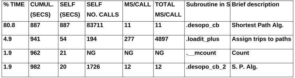
Table 1 gives a detailed profile of the four most time consuming routines, categorised by the percentage of CPU time used while running the computationally intensive SATALL program, when applied to a sample problem supplied by the Dublin Transportation Office (DTO). The first column, ‘% Time’, gives the percentage of CPU time that each routine uses while SATALL runs through a given problem. The next column gives the cumulative time used up by successive routines as the model iterates for each of the four routines shown. Column three gives the time that each routine uses itself, as opposed to the additional time spent in routines that are called from that routine. The column, ‘self calls’, gives the number of times that each routine is called from another routine while the next two give the milliseconds used within each routine per call and the total milliseconds used per call, including the time spent in subroutines that are called from the main routines.
% TIME CUMUL.
(SECS)
SELF
(SECS)
SELF
NO. CALLS
MS/CALL TOTAL
MS/CALL
Subroutine in S Brief description
80.8 887 887 83711 11 11 .desopo_cb Shortest Path Alg.
4.9 941 54 194 277 4897 .loadit_plus Assign trips to paths
1.9 962 21 NG NG NG .__mcount Count
[image:6.595.69.563.485.617.2]1.9 982 20 1726 12 12 .desopo_cb_2 S. P. Alg.
Table 1: Profile of CPU related figures and number counts for routines within the
SATALL program
shortest paths) uses 5% of the total CPU time. This only leaves approximately 12% of the overall running time for all of the other routines that make up the program SATALL. The details for these routines are not shown in Table 1, as there are too many of them to list. Since both the “desopo_cb” and the “loadit_plus” routines are both part of the assignment, and because these routines give the assignment over 85% of the overall CPU running time for SATALL, it was decided that the assignment should be targeted for further research.
2.2 Shortest Path Algorithms
The method for building a minimum path tree, or shortest path tree, may be described simply using the following general notation:
• The length of a link between two nodes, A and B, in the network is LA,B;
• The length of the chosen path is the sum of the link lengths in the path;
• The minimum distance from the origin, O, to the node A is LA; and,
• The back-node of A is BA and the link (BA, A) is a part of the shortest path.
Set-up:
• Set all LA = ∞, LO = 0 and all BA equal to some default value;
• Set up a loose-end table T to contain nodes, Ti, already reached by the algorithm but
not fully analysed as back-nodes for further nodes. Entries into this table represent the outer ends of the tree as branches grow to connect all of the nodes together; and, • All entries are set to zero, Ti = 0.
Method:
Starting with the origin, ‘O’, equal to the ‘current node’, A;
(1) Look at each link (A, B) from the ‘current node’, A, in turn and if LA + L(A,B) < LB then
set LB = LA + L(A,B), set BB = A, and add B to the loose-end table, T, provided that B is
(2) Remove A from T and if the table is empty, stop. Otherwise continue to step (3); and, (3) Select another node from the table and return to step (1) with it as the ‘current node’ A. Once this process has come to an end then LA contains the set of minimum lengths, measured
using costs, distances or by other means, from the origin, O, to each node or centroid, A. The back-node, BA, then contains all of the data necessary to retrace all of the shortest paths.
A number of classical algorithms exist which solve the shortest paths problem within the field of transportation. These include the Bellman-Ford-Moore algorithm [5, 26, 53], algorithms due to Moore [53], Dijkstra [22], Pallottino [58] and the D’Esopo-Pape algorithm, as described and tested by Pape [61] while being credited to D’Esopo by Pollock et al. [62]. A number of reviews exist on shortest path algorithms in general, for example see, amongst others, Deo and Pang [19], Gallo and Pallottino [28], Bertsekas [7], Ahuja et al. [2] and Cherkassky et al. [16], and within transportation models see, Van Vliet [73] and Gallo and Pallottino [29]. It is recognised that these algorithms have all developed using different strategies for selecting labelled nodes to be scanned in order to solve the single-source shortest paths problem on transportation networks and other sparse networks [43, 31, 28, 32].
The basic label-setting algorithm is due to Dijkstra [22]. In label-setting algorithms the node with the smallest distance label is removed from the list during each iteration. If the costs of travelling from node ‘i’ to node ‘j’ are non-negative then the removed node will never enter the list again. Label-correcting algorithms, on the other hand, do not necessarily remove the node whose label is the minimum. Hence, a node that has been removed may re-enter the list at a later time. Label-correcting algorithms have been shown to have better experimental performance than label-setting algorithms for sparse networks [43, 42, 28, 33, 61].
To examine the performance difference between label-correcting and label-setting two of the main algorithms in the field of transportation for solving the shortest path problem, those due to Moore and Dijkstra, are compared. The main difference between these algorithms lies in the procedure for selecting a labelled node from the loose-end table. Moore’s algorithm is a label-correcting algorithm, and Dijkstra’s algorithm is a label setting algorithm. Moore selects the top entry on the loose-end table, which is the oldest entry in the table. On the other hand, Dijkstra selects the node that is nearest to the origin, which requires additional computation but it does ensure that each node is examined only once. It is well known, according to Ortuzar and Willumsen [56], that Dijkstra’s algorithm is superior to Moore’s, especially for large networks, although it is more difficult to program. However, the D’Esopo extension to Moore’s algorithm has been found by Van Vliet [72, 73] to be both more efficient and faster over a range of sparse transportation network sizes and configurations.
small networks by Van Vliet [73]. The D’Esopo algorithm is an extension to Moore’s algorithm in that it uses a two-ended lose-end table, also known as a deque list (double-ended queue) for which additions and deletions are possible at either end, so that a node is entered at one of the ends depending on its status. In this way any node that has already been examined but comes up again as the algorithm progresses is immediately examined again because it will have been stored at the top of the loose-end table; see Van Vliet [72] and Pape [61] for more detail.
As shown by Van Vliet [72], the D’Esopo algorithm can reduce CPU times by up to 50 % when compared to Moore’s algorithm. Furthermore, from a similar study made by Van Vliet [73] of these algorithms, over a wide range of network sizes and configurations, the D’Esopo modification to Moore’s algorithm gives minimum CPU times when compared with those times obtained from the best implementations of Dijkstra’s algorithm, which used a box-sort in 1977.
It is concluded that when dealing with the shortest path problem in the SATURN model this research will concentrate on the parallelisation of the D’Esopo algorithm for the following reasons:
(1) In the case of transportation models, networks generally have nonnegative arc costs and structured sparse graphs. Therefore, the current deque shortest path algorithm, i.e., the D’Esopo algorithm, seems to be the best choice of algorithm for transportation applications, excluding specific circumstances where specialised algorithms need to be used [29, 59].
(2) The robustness of the D’Esopo algorithm relates to it being able to solve the shortest paths problem for different network sizes and configurations more efficiently than both Moore, which is only faster for very small networks (less than 75 nodes) and Dijkstra (box-sort), which is only faster for large networks with short nonnegative link lengths [73].
2.3 Parallel programming in traffic assignment and shortest path theory
2.3.1 Assignment
dedicated to the co-ordination of the activities of the slave processors and to their communication requirements. An approach by Hislop et al. [40], where the network is dissected into zones and traffic is assigned to the zones in parallel, was discarded because of the difficulties with assigning ‘packets’ to cross-boundary routes. It was decided that a simpler data decomposition strategy to assign all ‘packets’ in parallel was more appropriate. This resulted in a speed-up of nine times using 16 T805 Transputers for a network of 1001 links.
Chabini et al. [14] looked at parallel and distributed computation of shortest routes and network equilibrium models. They present parallel computing implementations of the linear approximation method for solving the fixed demand network equilibrium problem. Chabini et al. [14] also contains parallel computing implementations of a shortest paths algorithm due to Dijkstra [22]. The linear approximation method used to solve the fixed demand network equilibrium problem by Chabini et al. [14], is an adaptation of the Frank-Wolfe algorithm [27, 4]. In the sequential implementation of this algorithm a variant of Dijkstra’s [22] algorithm is used to calculate shortest routes for all origin-destination pairs. The methodology used to parallelise Dijkstra’s algorithm by Chabini et al. [14] is also a master-slave decomposition model.
and for solving the fixed demand network equilibrium problem on the computing platforms and environments that were available at the time.
Nagel and Rickert [54] make use of the master-slave approach using decomposition for a parallel implementation of the TRANSIMS micro-simulation. Reference is also made to Chabini [13] where domain decomposition is used to partition the network graph into domains of approximately the same size for a discrete dynamic shortest path problem.
2.3.2 Single-source one-to-all shortest path parallel algorithms
The majority of work that has taken place has focused on developing and comparing different parallel implementations for sequential label-setting and label-correcting algorithms [43]. A number of parallel algorithms have been proposed for various sequential shortest path algorithms such as those documented by Tseng et al. [71], Paige and Kruskal [57] and Chandy and Misra [15] on machine independent algorithms and those by Habbal et al. [38] and Dey and Srimani [21] on machine specific algorithms. The most investigated area being the all– pairs problem, see Habbal et al. [38], Paige and Kruskal [57], Chandy and Misra [15] and Deo et al. [20]. Several attempts have been made to parallelise the single source shortest path problem but with relatively little success [69, 9, 57, 20], however, certain adaptations of Moore’s algorithm seem promising according to Deo et al. [20].
By 1991, parallel algorithms for finding the shortest paths within the field of transportation were based on Dijkstra, Moore and D’Esopo, and, Dynamic Programming [40]. Bitz and Kung [12] distributed Dynamic Programming on an iWarp systolic array but found that the method did not perform well on large networks. Mateti and Deo [49] give examples of distributing Dijkstra’s and Moore’s algorithms on a shared memory MIMD machine and on a specialised vector addition and comparison supercomputer.
synchronous implementation with measures included to reduce the communication costs, performed well. Experimental studies of distributed label-setting algorithms, such as those by Traff [69] and Adamson and Tick [1], use a partition of the network among processors so that each processor has its own sub-network on which to work. It was observed that label-setting algorithms have little parallelism [43]. Crauser et al. [17] also describe a theoretical approach to parallelising Dijkstra’s algorithm by dividing the algorithm into a number of phases to be executed in parallel, a method of process decomposition. The implementation shows good theoretical behaviour and further research is recommended. Bertsekas and Tsitsiklis [10] have surveyed both synchronous and asynchronous iterative algorithms with mixed convergence results. Traff [69] also found that for distributed memory systems achieving speedup for Moore’s algorithm is ‘apparently’ easier than for Dijkstra’s.
compare it to a sequential implementation of the Bellman-Ford-Moore algorithm developed by Cherkassky et al. [16].
Ziliaskopoulos et al. [84] introduces parallel designs for the dynamic time-dependent least time path algorithms using shared memory and message passing approaches. The parallel algorithms are based on sequential dynamic algorithms introduced by Ziliaskopoulos and Mahmassani [83, 81] using discrete time steps and the theory of Bellman’s principle of optimality. However, no testing was carried out on large networks. This research is continued through Ziliaskopoulos and Kotzinos [80] who propose and execute a massively parallel design for the time-dependent least time path algorithm, which is also based on sequential work by Ziliaskopoulos and Mahmassani [83, 81], on a PVM system. While speedup improves with the number of time intervals it is also acknowledged that further research into efficiency, over actual and random networks, is necessary.
path problem using labelling algorithms on distributed memory machines. This takes advantage of the aggregate memory of the distributed system and parallelism can exceed the number of sources. However, there are high communication overheads associated with communicating node labels, and for termination detection [43].
3. Methodology
The major objective for the parallelisation of the SATURN model was to improve the model’s performance so as to be able to apply the model to computationally intensive, and hence time intensive, transportation problems that otherwise might not be assessed. The strategy for programming the SATURN model in parallel is to take the most CPU computationally intensive components of the model (calculation of the shortest paths) and to parallelise this section in such a way that the resulting parallel version of the model converges, is accurate, has a more efficient performance and is portable.
3.1 Strategy
Any parallel version of SATURN [75] shall, in modifying the relevant algorithms and code, ensure that the parallel model can be used on a number of different systems with a minimum of difficulty. Although this research will be applying the parallel solution on an IBM RS/6000 SP2 supercomputer, the final solution will be compatible with most parallel systems. The IBM SP2 has 48 Power2SC processors, although only 16 were utilised in this research due to administrative restrictions as a result of the workload on the machine; see Section 4 for a description of the system. In order to do this the solution has been designed to be compatible with both distributed memory and shared memory systems.
or output (I/O) channels. This is known as the communication sequential process model [14] for parallel execution, which was initially developed by Hoare [41] in the 1970’s and is the basis for the message passing paradigm. This model is commonly used in communication libraries such as, for example, the MPI interface [50, 76]. Two basic functions, called ‘send’ and ‘receive’, are generally used to send and receive the information along channels between processes.
PVM is a system designed for managing and coordinating parallel systems. It was produced by researchers at Emory University, the University of Tennessee, Knoxville, and Oak Ridge National Laboratory as a research development project [30, 66]. When the development of the MPI interface began PVM was the most popular message passing system in use. It has been regarded that MPI and PVM have been competing to become the message passing standard since then, however, two of PVM’s principle developers, Jack Dongarra and Al Geist, were also key to the development of MPI [39].
The design objectives for MPI and PVM differed greatly. PVM was designed for use on networks of workstations and problems to do with interoperability and resource management. As a result its message passing facilities are not very sophisticated. In contrast, MPI’s development focused on message passing and is intended to provide high performance on tightly-coupled homogeneous parallel computing architectures, which it has achieved [39]. Gropp and Lusk [34] also provide a comparison between PVM and MPI finding MPI more credible than other message passing libraries because of the consultative process involved in its creation. Development of message passing aspects of PVM were stopped after Version 3.4 in favour of research into distributed, heterogeneous environments for networks of workstations while some of PVM’s major strengths, such as its resource management capabilities, have been incorporated into MPI. Today the majority of parallel computer producers support MPI as their primary message passing interface with other interfaces available for reasons of compatibility with legacy codes [39].
platform and threads. The drawback of the shared memory version is the limited scalability. Most shared memory systems are more expensive and use fewer processors than distributed systems. At some stage further processors cannot be used as the contention between processors in trying to access the memory at the same time becomes too large. Supercomputers such as the CRAY range can cost millions of dollars for onsite installation but can take existing sequential programs written in computer languages such as C, C++ and FORTRAN and convert the code so that it can run in parallel on the machine with minimal effort on the behalf of the programmer. MIMD machines are far cheaper and offer far greater flexibility in the way problems are distributed, examples being transputers and distributed networks of workstations. However, they are harder to set-up and program in parallel [40]. An example of a SIMD machine is the CM-2 connection machine, see Zenios [78]. The majority of parallel systems becoming available belong to the MIMD category however [3].
3.2 Parallel programming, shortest paths and assignment
The shortest path problem has been shown to take up over 80 percent of the overall CPU time for SATALL. For every origin in the network a shortest path is found to every possible destination so the same computations are made to achieve a shortest path for every Origin-Destination (O-D) pair. In programming the shortest path problem in parallel a simple decomposition by origin is used where the total number of origins is divided into a number of subtasks in such a way that each subtask can be issued to a separate processor for analysis. Each subtask then corresponds to the computation of a subset of the total number of origins and has the same code as all the other subtasks. The label-correcting single-source D’Esopo modification to Moore’s algorithm is being used as the shortest path algorithm of choice. Though not the fastest algorithm for specific network sizes and configurations the algorithm performs very well over a wide range of transportation applications unlike other well known algorithms such as Dijkstra’s label-setting algorithm, which needs to be invoked in different ways to achieve good performance depending on the specific circumstances. Chabini et al. [14] has found that a slow sequential algorithm can lead to very good speedups when the serial version of the algorithm is coded and the computation of shortest paths is shared for subsets of origins among processors.
From a software perspective, the use of partition in decomposition consists of determining the size of each of the subtasks to be assigned to each processor. Depending on the resulting size of each subtask three levels of parallelisation are produced; fine, medium and coarse-grained. In fine-grained parallelism each subtask can represent an operating instruction, as compared to coarse-grained parallelism where each subtask can represent a procedure or loop. In order to do this other criteria must also be considered. Allocation looks at assigning each subtask to a processor so that priority constraints amongst subtasks are respected. Load balancing is tightly interconnected with allocation and partition. The main objective of load balancing is to keep all the processors in use, as far as is practicable, and equally loaded in terms of the execution times of the processes allocated to them. Fine-grained subtasks are useful for load balancing but can result in an increase in communication overheads. Coarse-grained subtasks can result in long idle times for processors that have finished their subtask and are waiting for other processors to finish so that the algorithm can continue in a synchronised manner.
The main problem with parallelising the single source shortest path problem is that the problem is inherently sequential with a large number of iterations taking short periods of time, yielding very small grain sizes. One way to overcome this problem is to perform more computations within each subtask, so as to increase the grain size [84].
terms of computation and can run in parallel without having to communicate very often with other subtasks also running in parallel. This reduces the inefficiencies associated with communication overheads, which would be incurred in a fine-grained parallelisation as subtasks running in parallel would have to communicate more frequently; see Chabini [13] for more detail of fine-grained parallelism in shortest path theory. Creating these subtasks is achieved by dividing the total number of origins by the number of processors being used for the implementation, an early implementation of which is due to Chabini [14]. The result is that there is a very high ratio of ‘computational execution to data input’, which is what allows distribution of the sequential code and a parallelisation approach based around the shortest path loop instead of inside the shortest path algorithm.
Hislop et al. [40], which is limited by the computational bottleneck inherent in a centralised system arising from traffic levels, or the transportation network, becoming too large.
4. Results and Discussion
A number of different samples were analysed on three different platforms. Comparisons were then drawn between outputs from the parallel model and outputs from the sequential model on each system. The machines that were used were the Intel dual processor i686, the IBM RS/6000 F50 (4-processor) SMP shared memory system and the IBM RS/6000 Scalable POWERParallel SP2 supercomputer.
The IBM RS/6000 SP2 System is a distributed memory multi-processor parallel system composed of processor nodes. Each node contains a single Power2SC processor running at 160MHz and runs its own copy of the AIX V4.3.3 operating system. Its peak performance is 640 MFLOPS with 4 FP results/clock, an L1 Instruction Cache of 32 K and an L1 Data Cache of 128 K. The memory configuration is as follows:
• Node 01 >> node 16: 1 GB memory; • Node 17 >> node 26: 512 MB memory;
• Node 27 >> node 48: 256 MB memory.
The total peak performance of the system is 30GFlops. The nodes are connected together using the High Performance Switch Omega Network. For this research 256MB of memory were assigned, as a minimum, to the execution of the program per processor.
instruction cache of 32 K, L1 data cache of 32 K, L2 cache of 256 KB and an L2 associativity of one.
The GDA trip matrix has 432 fine zones, with finer zones in the City Centre and coarser zones further out, giving 432 sources (O-Ds). The highway network is made up of a simulation network and a buffer network, combining to give over 1,220 simulation nodes (junctions) and 3,900 links throughout the GDA. The model uses up approximately 1.5 MB of space when running on each processor; this was found using the AIX command ‘TOP’. Convergence and accuracy were assessed over smaller sample networks before the parallel model was run for the entire Greater Dublin Area until convergence was reached.
4.1 Convergence
The parallel model was run on both parallel systems and sequentially over a single processor. Convergence was reached after the same number of iterations for all model runs. Once it was clear that the parallel model converged the output was compared to that of the sequential SATURN model. ISTOP is a percentile convergence parameter that stops the loop between the simulation and assignment from continuing if ‘ISTOP’ percentage of the link flows change by less than a predefined value, 5 percent in this case. After the 15th loop the following output is produced for the parameter ISTOP where ISTOP is set equal to 90%.
• For the SATURN model run on the IBM ibix machine, using one processor, 89.8 percent of
the assigned flows are within 5% of their values from the previous simulation/assignment iteration.
• For the i686 dual processor machine, using two processors, 90.7% of the assigned flows are
• For the IBM ibix machine, using four processors, 91.3% of the assigned flows are within
5% of their values from the previous simulation/assignment iteration.
This demonstrates that the parallel model converges with the same or greater accuracy than the sequential SATURN model. This has been found to hold for any number of processors that have been used, up to and including 16 processors. It is noted that ISTOP is converging more quickly as more processors are used although the authors recognise that ISTOP gives a strong indication of convergence but does not give proof of convergence. In the first case above, using the IBM ibix machine, the model has not converged on the 15th loop as only 89.8% of the assigned flows are within 5%. This means that it will have to go through a 16th loop to converge, hence adding a considerable amount of time to the overall running time of the model.
There are no apparent reasons for the differences in the rates of convergence viewed above as the convergence theory remains unchanged for the parallel application. However, the trend, as small as it appears to be, persists leading to the tentative conclusion that perhaps the decomposition of origins has a deterministic effect on the convergence theory of the model or, perhaps, an explicit effect on the numerical computation of convergence itself. Further research is necessary to establish what effect, if any, there appears to be.
4.2 Comparison of Model Outputs
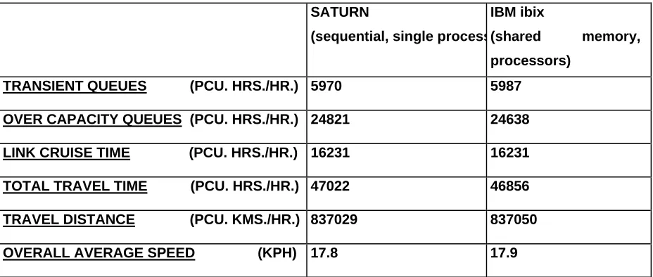
less than one percent, as demonstrated in Table 2 below. In practice the accuracy of the model output has been found to hold for any number of processors that have been used, up to and including 16 processors on the IBM SP2.
SATURN
(sequential, single process
IBM ibix
(shared memory,
processors)
TRANSIENT QUEUES (PCU. HRS./HR.) 5970 5987
OVER CAPACITY QUEUES (PCU. HRS./HR.) 24821 24638
LINK CRUISE TIME (PCU. HRS./HR.) 16231 16231
TOTAL TRAVEL TIME (PCU. HRS./HR.) 47022 46856
TRAVEL DISTANCE (PCU. KMS./HR.) 837029 837050
[image:28.595.88.552.153.350.2]OVERALL AVERAGE SPEED (KPH) 17.8 17.9
Table 2: Sequential SATURN output compared with parallel model output.
Once the accuracy and convergence of the parallel model were determined the models performance was assessed.
4.3 Performance
The performance of a parallel computer system, combining a software element in the parallel algorithm and a hardware element in the parallel platform, needs to be assessed. The definition of performance depends on the reason behind the use of parallel programming in the first place. In general a reduction in the computation time of the program is sought. Hence, the improvement in performance is measured by comparing the sequential time to run the program on a single processor against that of the parallel application across a number of processors.
one processor and ‘n’ processors to solve a problem. It may also be interpreted as the average number of processors kept busy during the execution of the problem [14].
As more processors are assigned to the execution of a problem it is expected that the speedup will increase. However, it may also be expected that the total idle time will increase due to communication overheads between processors and processes, the software structure, and, contention between different components of the system for shared resources, i.e., two processors trying to access the same memory block at the same time in a share memory parallel computer [24]. Overheads due to I/O are, in the case examined here, not included in the assessment of the performance of the parallel system. The overheads, as described above, are said to be represented by including them in the service demands of the various subtasks. In this way one can assume that they are fixed and do not vary with the number of processors being used nor with the scheduling procedure for the subtasks [24].
The average parallelism measure was first introduced by Gurd et al. [37] in their review of the architecture and performance of the “Manchester Prototype Dataflow Computer”. They found that programs with a similar value of average parallelism exhibit virtually identical speedup curves and that the higher the value, the closer the program got to achieving 100 percent utilization, i.e., an efficiency of 1 on a graph. This seems to indicate that the measure of average parallelism is all that is necessary to ascertain an accurate description of its speedup curve, regardless of other factors such as the source code language, the time variance of parallelism, etc. Gurd et al. [37] also concluded that larger applications codes exhibited the same patterns as simpler samples. Eager et al. [24] give 4 definitions of the average parallelism, one of which is:
• The average number of processors that remain busy during the execution of a software
system given an unlimited number of available processors.
Profiles that plot benefit against cost are common in many areas. The concept of there being a ‘knee’ in such a profile is a fundamental one, see Denning [18]. The ‘knee’ is the point where the benefit per unit cost is maximised. The execution time-efficiency profile is one such cost-benefit profile in parallel systems. Eager et al. [24] give two motivational stand points for the use of this graph in parallel systems:
(1) Efficiency is viewed as an indication of benefit (as efficiency goes up so does benefit) and execution time as an indication of cost (as execution time goes up so does cost). The system objective that can be taken from this is to achieve efficient usage of each processor while taking into account the cost to users in the form of increased execution times.
higher the cost). The objective that can be taken from this is to achieve low execution times while taking into account the utilization cost of low efficiency.
N, the number of processors used to run the model
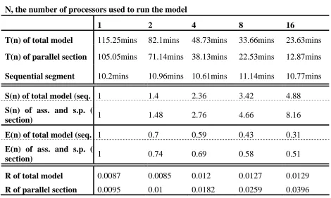
1 2 4 8 16 T(n) of total model 115.25mins 82.1mins 48.73mins 33.66mins 23.63mins
T(n) of parallel section 105.05mins 71.14mins 38.13mins 22.53mins 12.87mins
Sequential segment 10.2mins 10.96mins 10.61mins 11.14mins 10.77mins
S(n) of total model (seq. i1 1.4 2.36 3.42 4.88
S(n) of ass. and s.p. (
section) 1 1.48 2.76 4.66 8.16
E(n) of total model (seq. 1 0.7 0.59 0.43 0.31
E(n) of ass. and s.p. (p
section) 1 0.74 0.69 0.58 0.51
R of total model 0.0087 0.0085 0.012 0.0127 0.0129
[image:32.595.83.553.102.384.2]R of parallel section 0.0095 0.01 0.0182 0.0259 0.0396
Table 3: The time taken to complete the parallel model on the SP2 machine, with and
without the sequential section; the speed-up, S(n); the efficiency, E(n); and the ratio of
efficiency to execution time, R.
point but if one more processor is added then it would be utilized no more than 50 percent. It is further shown that the location of the ‘knee’, i.e., the number of processors used at this location, is well approximated by the average parallelism, where the same guarantees regarding speedup and efficiency are identical to those at the ‘knee’.
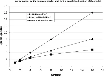
“Optimum Performance”. This graph was produced by solving the GDA trip matrix assignment/simulation problem using 1, 2, 4, 8 and 16 processors. More processors were not used because of administrative limitations due to large system demand and workload.
It is noted from Table 3 and Figure 1 that while the speed-up for the complete model drops off quickly with a value of 4.88 for 16 processors, the performance of the parallel section of the model is far better with a value of 8.16 for 16 processors. The obvious reason for this is that the sequential section of the parallel model takes the same amount of time to complete no matter how many processors are being used. This is reinforced by examining the efficiency of the model. The efficiency, E(n), of the model decreases quickly as the relative importance of the sequential section increases. The sequential section represents 9 percent of the execution time, T(n), of the model using 1 processor but it represents 54 percent when 16 processors are used. As such the sequential nature of the model represents the dominant limiting factor in the parallel implementation.
It is also noted that the efficiency, E(n), execution time, T(n), profile of the model, represented by the ratio of one to the other, R, while still increasing for 16 processors at 0.0129, appears to be levelling off quite quickly. This is expected due to the sequential section, however it does suggest that the ‘knee’ of the model, as described earlier, lies somewhere around 0.013. This point gives a reasonably accurate location for the average parallelism of the model as described earlier.
conclusion that the number of processors needed to reach the ‘knee’ for the parallel section is far more than is available for this research. Examining Figure 1 it is noted that for the parallel section, after an initial drop in performance from 1 to 2 processors, the performance recovers and an almost linear relationship is noted for 4, 8 and 16 processors. The rate of decrease of the efficiency is reducing and the ratio, R, suggests that the pattern of the graph will continue for a considerable number of extra processors.
NPROC, the number of processors used to run the model
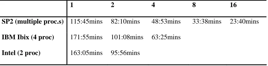
1 2 4 8 16
SP2 (multiple proc.s) 115:45mins 82:10mins 48:53mins 33:38mins 23:40mins
IBM Ibix (4 proc) 171:55mins 101:08mins 63:25mins
[image:35.595.87.553.129.245.2]Intel (2 proc) 163:05mins 95:56mins
Table 4: The time taken to complete the parallel model, with the sequential section and
I/O included, for the three systems analysed.
the SP2 machine, which far exceeds that of the shared memory Ibix machine or the dual processor Intel machine. The times shown in Table 4, in minutes, give the total time taken for the model run to completion using three different machines over 1, 2, 4, 8 and 16 processors.
Using just one processor the SP2 machine takes approximately 115 minutes as compared to that of 172 minutes and 163 minutes for the Ibix and Intel computers respectively. Using 8 or 16 processors the time is 3.4 and 4.9 times faster than a single processor respectively. The time of 23.66 minutes for the SP2 machine to complete the model run using 16 processors saves 92 minutes when compared to the time taken for a single processor and saves 148 minutes and 139 minutes when compared to the time taken for a single processor to finish the job on the Ibix and Intel respectively.
5. Conclusions
• The parallel model is converging accurately and at the same rate, as expected, when
compared to that of the sequential SATURN model. However, it also appears that as more processors are used convergence occurs more quickly than with the sequential model, though the difference in convergence performance is not particularly significant and is most likely incidental, further research could be undertaken to determine any abstract effects from the parallelisation process. For a more viable improvement in the convergence performance itself perhaps research on the model algorithms themselves would be more useful.
• The ISTOP number was used in the research to give an indication of performance but
further work would be required to investigate a mathematical proof that the parallel algorithm will converge.
• The output from the parallel model is within one percent of the results from the sequential
model for the scenarios tested over a number of runs.
• The speed-up of the model (including the sequential section and the parallel section)
against the number of processors being used is approximately 80% of the CPU time for the sequential model. The speed-up of the total parallel model is approximately equal to 5 for the program running over 16 processors. However, if one does a similar comparison but only looking at the parallelised module an increase in speed-up to approximately 8.16 is found for 16 processors.
• The most computationally intensive part of the SATURN code has been successfully
within the field that any attempt to parallelise the shortest path algorithm itself is unlikely to prove worthwhile from a performance standpoint.
References
1. Adamson, P. and E. Tick, Greedy partitioned algorithms for the shortest path problem, International Journal of Parallel Programming, Vol. 20, 271-298, 1991.
2. Ahuja, R. K., Magnanti, T. L., and J. B. Orlin, “Network Flows”, Theory, Algorithms and Applications, Prentice-Hall, 1993.
3. Allsop, R. E., Guest Editorial, Transportation Research C, Vol. 5, No. 2, 73-76, 1997.
4. Arezki Y. and D. van Vliet, A full analytical implementation of the PARTAN/Frank-Wolfe algorithm for equilibrium assignment, Transportation Science, Vol. 24, No. 1, 58-62, Feb. 1990.
5. Bellman, R., On a routing problem, Quarterly Applied Mathematics, Vol. 16, 87-90, 1958.
6. Bertsekas, D. P., An auction algorithm for shortest paths, SIAM Journal on Optimization, Vol. 1, 425-447, 1991.
7. Bertsekas, D. P., “Linear network optimization: Algorithms and codes”, MIT Press, Cambridge, MA, 1991b.
8. Bertsekas, D. P. and D. A. Castanon, Parallel synchronous and asynchronous implementations of the auction algorithm, Parallel Computing, Vol. 17, 707-732, 1991.
9. Bertsekas, D.P. and J.N. Tsitsiklis, “Parallel and Distributed Computation”, PrenticeHall, Englewood Cliffs, 1989.
10. Bertsekas, D. P. and J. N. Tsitsiklis, Some aspects of parallel and distributed iterative algorithms - a survey, Automatica, Vol. 27, No. 1, 3-21, 1991.
11. Bertsekas, D. P., Guerriero, F., and R. Musmanno, Parallel asynchronous label-correcting methods for shortest paths, Journal of Optimization Theory and Applications, Vol. 89, No. 1, 1996. To appear.
12. Bitz, F. and H. T. Kung, Path Planning on the WARP Computer: Using a Linear Systolic Array in Dynamic Programming, International Journal of Computer Mathematics, Vol. 25, 173-188, 1988.
13. Chabini, I., Discrete dynamic shortest path problems in transportation applications: complexity and algorithms with optimal run time, Transportation Research Record, 1645, 170-175, 1998. 14. Chabini, I., Florian, M. and E. Le Saux, “Parallel and Distributed Computation of Shortest
Routes and Network Equilibrium Models”, Dept. of Civil and Environmental Engineering, MIT, Cambridge, MA 02139-4307, U. S. A., 1997.
15. Chandy, K. M. and J. Misra, Distributed Computation on Graphs: Shortest Path Algorithms, Comm. ACM, Vol. 25, 833-837, 1982.
16. Cherkassky, B. V., Goldberg, A. V. and T. Radzik, Shortest path algorithms: Theory and experimental evaluation, Mathematical Programming, Vol. 73, 129-174, 1996.
17. Crauser, A., Mehlhorn, K., Meyer, U., and P. Sanders, “A parallelization of Dijkstra's shortest path algorithm”, in 23rd Symposium on Mathematical Foundations of Computer Science, LNCS, Brno, Czech Republic, Springer, 1998.
18. Denning, P. J., Working Sets Past and Present, IEEE Transactions on Software Engineering, SE Vol. 6, No. 1, 64-84, January 1980.
19. Deo, N. and C. Pang, Shortest path algorithms: Taxonomy and annotation, Networks, Vol. 14, 275-323, 1984.
21. Dey, S. and P. K. Srimani, Fast parallel algorithm for all-pairs shortest path problem and its VLSI implementation, IEE Proceedings, Vol. 136, Pt. E, No. 2, March 1989.
22. Dijkstra, E. W., A note on two problems in connection with graphs (spanning tree, shortest path), Numerical Mathematics, Vol. 1, 269-271, 1959.
23. Dublin Transportation Initiative, “Final Report, Technical Annex on Transportation Modelling”, Department of the Environment, Dublin, 1995.
24. Eager, D. L., Zahorjan, J., and E. D. Lazowska, Speedup versus efficiency in parallel systems, IEEE Transactions on Computers, Vol. 38, No. 3, 408-423, 1989.
25. Florian, M., Applications of parallel computing in transportation: Guest editorial, Parallel Computing, Vol. 27, 1521-1522, 2001.
26. Ford, L. R. and D. R. Fulkerson, Maximal flow through a network, Flows in Networks, 399-404, Princeton University Press, 1962.
27. Frank M. and P. Wolfe, An algorithm for quadratic programming, Naval Research Logistics Quarterly, Vol. 3, 95-110, 1956.
28. Gallo, G. and S. Pallottino, Shortest Path Methods: A Unifying Approach, Mathematical Programming Study, Vol. 26, 38-64, 1986.
29. Gallo, G. and S. Pallottino, Shortest path methods in transportation models, in (M. Florian, ed.), Transportation planning models, North-Holland, 227-256, 1984.
30. Geist, A., Beguelin, A., Dongarra, J., Jiang, W., Manchek, B. and V. Sunderam, “PVM: Parallel Virtual Machine---A User's Guide and Tutorial for Network Parallel Computing”, MIT Press, 1994.
31. Goldberg A. V. and T. Radzik, A heuristic improvement of the Bellman-Ford algorithm, Applied Mathematics Letters, Vol. 6, 3-6, 1993.
32. Golden, B., Shortest-path algorithms: A comparison, Operations Research, Vol. 24, No. 6, 1164-1168, 1976.
33. Greenwood, D. G. and N. B. Taylor, “Parallelising the CONTRAM traffic assignment model”, in 1993 European Multi-simulation Conference, Lyon, 7-9, June 1993.
34. Gropp, W. and E. Lusk, “Why Are PVM and MPI So Different?”, in: Bubak, M., Dongarra, J. (Eds.): Recent Advances in PVM and MPI, LNCS, Vol. 1332, Springer- Verlag, Berlin Heidelberg New York, 3-10, 1997.
35. Gropp W., Lusk, E., and A. Skjellum, “Using MPI – Portable Parallel Programming with the Message-Passing Interface”, The MIT Press, Cambridge, MA, London, England, 1994.
36. Gropp, W., Huss-Lederman, S., Lumsdaine, A., Lusk, E., Nitzberg, B., Saphir, W., and M. Snir, “MPI: The Complete Reference Volume 2 - The MPI-2 Extension”, MIT Press, 1998.
37. Gurd, J., Kirkham, C.C. and I. Watson, The Manchester Prototype Dataflow Computer, Communications of the Association for Computing Machinery, Vol. 28, No. 1, 34-52, January 1985.
38. Habbal, M., Koutsopoulos, H. and S. Lerman, A decomposition algorithm for the all-pairs shortest path problem on massively parallel computer architectures, Transportation Science, December 1994.
39. Hempel, R. and D. W. Walker, The emergence of the MPI message passing standard for parallel computing, Computer Standards and Interfaces, Vol. 21, 51-62, 1999.
40. Hislop, A. D., McDonald, M. and N. Hounsell, The application of parallel processing to traffic assignment or use with route guidance, Traffic Engineering and Control, 510-515, Nov. 1991.
41. Hoare, C. A. R., Communicating Sequential Processes, Communications of the ACM, Vol. 21, No. 8, 666-677, Aug 1978.
43. Hribar, M. R., Taylor, V. E. and D. E. Boyce, Implementing parallel shortest path for parallel transportation applications, Parallel Computing, Vol. 27, 1537-1568, 2001.
44. Hribar, M. R., Taylor, V. E. and D. E. Boyce, Termination detection for parallel shortest path algorithms, Journal of Parallel and Distributed Computing, Vol. 55, 153-165, 1998.
45. Kumar, V. and V. Singh, Scalability of Parallel Algorithms for the All-Pairs Shortest Path Problem, Journal of Parallel and Distributed Processing, Vol. 13, No. 2, 124-138, October 1991.
46. Lee, G., Kruskal, C. P. and D. J. Kuck, An Empirical Study of Automatic Restructuring of Nonnumerical Programs for Parallel Processors, Special Issue on Parallel Processing of IEEE Transactions on Computers, Part C, Vol. 34, No. 10, 927- 933, Oct. 1985.
47. Leonard, D. R. and P. Gower, “User Guide to CONTRAM Version 4”, TRRL Supplementary Report 735, Transport and Road Research Laboratory, Crowthorne, 1982.
48. Leonard, D.R., Gower, P., and N.B. Taylor, “CONTRAM: Structure of the Model”, TRL Report RR178, Transport Research Laboratory, Crowthorne, UK, 1989.
49. Mateti, P. and N. Deo, Parallel Algorithms for the Single Source Shortest Path Problem, Computing, Vol. 29, 31-49, 1982.
50. Message Passing Interface Forum, MPI: A Message Passing Interface Forum, International Journal of Supercomputer Applications and High Performance Computing, Vol. 8, No. 3/4, 165-414, 1994.
51. Minsky, M. and S. Papert, “On some associative, parallel and analog computations”, in Associative Information Technologies, E. J. Jacks, Ed., New York: Elsevier North Holland, 1971.
52. Mondou, J.F., Crainic, T.G. and S. Nguyen, Shrotest Path Algorithms: A Computational Study with C Programming Language, Computers and Operations Research, Vol. 18, 767-786, 1991.
53. Moore, E.F., “The shortest path through a maze”, in Proceedings of an international symposium on the theory of switching, 285-292, Harvard University, 1957.
54. Nagel, K. and M. Rickert, Parallel implementation of the TRANSIMS micro-simulation, Parallel Computing, Vol. 27, No. 12, 1611-1639, 2001.
55. Narayanan, P., “Single source shortest path problem on processor arrays”, in Proceedings Frontiers of Massively Parallel Computation, 553-556, McLean, VA, Oct. 1992.
56. Ortuzar, J. de D. and L. G. Willumsen, “Modelling Transport”, John Wiley and Sons Ltd., England, 1994.
57. Paige R. C. and C. P Kruskal, Parallel algorithms for shortest path problems, in IEEE, 14-20, 1985.
58. Pallottino, S., Shortest path methods: Complexity, interrelations and new propositions, Networks, Vol. 14, 257-267, 1984.
59. Pallottino, S. and M. Scutella, “Shortest path algorithms in transportation models: Classical and innovative aspects”, Technical Report: TR-97-06, Universit di Pisa, 1997.
60. Papaefthymiou, M. and J. Rodrigue, “Implementing parallel shortest-paths algorithms”, Department of Computer Science, Yale University, 1994.
61. Pape, U., Implementation and efficiency of Moore algorithms for the shortest route problem, Mathematical Programming, Vol. 7, 212-222, 1974.
62. Pollack, M. and W. Wiebenson, Solutions for the shortest route problem, Operations Research, Vol. 8, 224-230, 1960.
63. Polymenakos, L., and D. P. Bertsekas, Parallel Shortest Path Auction Algorithms, Parallel Computing, Vol. 20, 1221-1247, 1994.
64. Snir, M., Otto, S. W., Huss-Lederman, S., Walker, D. W., and J. Dongarra, “MPI: The Complete Reference”, Scientific and Engineering Computation Series, MIT Press, 1996.
66. Sunderam, V., PVM: A Framework for Parallel Distributed Computing, Concurrency: Practice and Experience, Vol. 2, No. 4, 315-339, December 1990.
67. Taylor, N.B., “CONTRAM 5: An enhanced traffic assignment model”, TRL Report RR249, Transport Research Laboratory, Crowthorne, UK, 1990.
68. Taylor, N.B., “Dynamic route guidance simulation with CONTRAM and ROGUS”, in Proceedings of PROMETHEUS Workshop on Traffic Related Simulation, Stuttgart, December 1992.
69. Traff, J. L., An experimental comparison of two distributed single-source shortest path algorithms, Parallel Computing, Vol. 21, 1505-1532, 1995.
70. Tremblay, N. and M. Florian, Temporal shortest paths: Parallel computing implementations, Parallel Computing, Vol. 27, 1569-1609, 2001.
71. Tseng, P., Bertsekas, D. P., and J. N. Tsitsiklis, Partially asynchronous, parallel algorithms for network flow and other problems, SIAM Journal of Control and Optimization, Vol. 28, 678-710, May 1990.
72. Van Vliet, D., D'Esopo: a forgotten tree-building algorithm, Traffic Engineering and Control, UK, July – August 1977.
73. Van Vliet D., Improved shortest path algorithms for transport networks, Transportation Research, Vol. 12, 7-20. Pergamon Press, 1978.
74. Van Vliet, D., SATURN – A modern assignment model, Traffic Engineering and Control, Vol. 23, No. 12, 578-581, Dec. 1982.
75. Van Vliet, D. and M. Hall, “SATURN 9.4 User Manual”, W.S. Atkins, UK, 1998.
76. Walker, D. W., The design of a standard message-passing interface for distributed memory concurrent computers, Parallel Computing, Vol. 20, No. 4, 657-673, 1994.
77. Wardrop, J. G., “Some theoretical aspects of road traffic research”, in Proceedings of the Institution of Civil Engineers, (Part II), Vol. 1, 325-378, 1952.
78. Zenios, S.A., Parallel numerical optimization: current status and annotated bibliography, ORSA Journal on Computing, Vol. 1, No. 1, 20-43, 1989.
79. Zhan, F. B. and C. E. Noon, Shortest Path Algorithms: An Evaluation using Real Road Networks, Transportation Science, Vol. 32, No. 1, 65-73, 1998.
80. Ziliaskopoulos, A. and D. Kotzinos, A massively parallel time-dependent least-time-path algorithm for intelligent transportation systems applications, Computer-Aided Civil and Infrastructure Engineering, Vol. 16, Issue 5, Special Issue: High Performance Computing, 337-346, 2001.
81. Ziliaskopoulos, A. K. and H. S. Mahmassani, A Note on Least Time Path Computation Considering Delays and Prohibitions for Intersection Movements, Transportation Research, Vol. 30, 1996, 359-367.
82. Ziliaskopoulos, A. and H.S. Mahmassani, “Design and implementation of a shortest path algorithm with time-dependent arc costs”, in Proceedings of the 5th Advanced Technology Conference, Washington, D.C., USA, 1072-1093, 1992.
83. Ziliaskopoulos, A. and H.S. Mahmassani, Time-Dependent, Shortest-Path Algorithm for Real-Time Intelligent Vehicle Highway System Applications, Transportation Research Record, Vol. 1408, 94-100, 1993.
Figure 1: Speed-up versus the number of processors used for the optimum performance, for the actual performance of the model, and, for the parallel section performance compromising the shortest path problem and assignment of flows.
Performance graph of Speed-up against the number of processors used, NPROC, for the ideal performance, for the complete model, and, for the parallelised section of the model.
0 2 4 6 8 10 12 14 16 18
0 2 4 6 8 10 12 14 16 18
NPROC
Speed-up, S(n)