Model Order Determination and
Characterisation of Direction of
Arrival (DOA) Estimators in the
Acoustic Context.
A dissertation submitted to the University of Dublin for the degree of Doctor of Philosophy
Angela Elizabeth Quinlan
Trinity College Dublin, October 2006
ii
Declaration
I hereby declare that this thesis has not been submitted as an exercise for a degree at this or any other University and that it is entirely my own work.
I agree that the Library may lend or copy this thesis upon request.
Signed,
Angela E. Quinlan
Summary
This thesis is concerned with the detection and characterization of acoustical sources using array signal processing techniques. In particular this work is concerned with deter-mining the number of sources present, and estimation of the Direction of Arrival (DOA) of the signals received by the array.
Firstly the problem of DOA estimation using array processing techniques is intro-duced and the possible applications of DOA estimation are discussed. The model of the wavefront propagating from the source to the array is recalled.
Chapter 2 provides the mathematical basis for the rest of the thesis. The mathematical estimation problem is introduced and the difficulties in finding an optimal estimator for DOA estimation are discussed.
A unified explanation and review of classical array processing DOA estimation tech-niques is then given. In particular the application of such techtech-niques to the problem of estimating the location of wideband sources is discussed. Recent developments in acous-tical source localisation are then reviewed.
The initial step in any estimation scheme is to determine the number of sources present. This process is called model order determination and classical model order determination methods are unsuited to situations where the number of snapshots available is small, however such situations frequently arise, particularly when dealing with non-stationary sources. Based on the profile of the noise eigenvalues of the observed data correlation matrix as introduced by Grouffaud et. al [1], a novel method of determining the number of acoustical sources present is presented. The performance of the proposed method is compared to classical model order determination techniques using both computer simula-tions and experimental recordings. In particular the effect of reverberation is considered. The proposed method is shown to outperform the classical methods while maintaining low computational complexity.
As it is not possible to find an optimal estimator for the DOA estimation problem, a sub-optimal estimator must instead be used. The choice of estimator depends on the characteristics of both the source and environment of the given estimation problem. Three of the most well known approaches to the DOA estimation problem are subspace-based estimation, in this case we consider the Multiple Signal Classification(MUSIC) algorithm, Maximum Likelihood (ML) estimation and Time-Delay Estimation (TDE) using the cross-correlation method.
iii
simulations and experimental recordings. Analysis of the Mean Square Error (MSE) of each of the estimators for decreasing SNR shows that all three estimators display a threshold SNR below which the MSE increases rapidly. This threshold determines the operational range of the estimators for the given estimation problem and is explained by examination of the behaviour of the estimators as the SNR is decreased. The effect of reverberation is considered by evaluating the performance of the methods for varying Useful-to-Detrimental U25 values. Comparison of the results found from each estimator
allows some conclusions to be drawn on the suitability of these estimation approaches for different localisation problems.
For any given localisation problem it is therefore of great practical importance to know the best possible performance that can achieved. Such knowledge allows for a decision to be made on whether or not starting from a given algorithm an improvement can be made, or whether or not the system performance requirements can ever be met. It is of particular importance to establish the threshold SNR value, as this value determines the operational range.
In this thesis the best performance that can be achieved by an estimator is evaluated using lower bounds on the Mean Square Error (MSE), allowing for prediction of the op-erating range of an estimator in a given situation. The best known of these bounds is the Cram´er-Rao Bound (CRB). Its popularity can be attributed to both its simplicity of calculation and the fact that asymptotically (high SNR and/or large number of samples) it is reached by the ML estimator. However, the CRB only provides an accurate indica-tion of achievable performance in the asymptotic (or small-error) region, as it does not predict the threshold effect. The resulting performance characterization may therefore be misleadingly optimistic.
For this reason the application of the Barankin Bound (BB), which is the greatest lower bound on the MSE of an unbiased estimator, is instead considered. Unfortunately however, it is generally not computable, and must therefore be approximated. In this thesis a practical means of classification of BB approximations is proposed. This classifi-cation scheme includes all previously existing approximation bounds, and highlights their underlying assumptions.
Acknowledgments
Firstly, I would like to thank my supervisor, Prof. Frank Boland for placing his trust in me to begin work in his new research group, and for his help throughout the course of my PhD. It is thanks to your powers of persuasion that I decided to do a PhD, and for this I am very grateful.
I would also like to express my gratitude to the examiners for the time and effort they put into exmaining this thesis.
I am also very grateful to the Irish Research Council for Science Engineering and Technology (IRCSET) for their generous funding of this work. In particular I would like to thank Dawn Carroll and Vicky Garnett of IRCSET, for their rapid help on any matters that arose throughout the course of my PhD.
I want to say a big thank you to the other post-graduate students and members of staff in the Electronics department in Trinity College for their help and friendship throughout the past few years. In particular I would like to thank Gavin, Deepti, Dennis and Damian for all their help and Francis for answering all those very important questions at the end. I also especially want to thank Claire for always helping me to see a funny side during the darker days!
It is hard to know where to begin to express my gratitude to the people in the ENS de Cachan, France. From the moment I arrived at the ENS you did all you could to make me feel at home. Benoit, Christoph, Stephanie, Francois, Mark, Leila, Ana, Eric Vourch, Ann, Dominique and the many many others. I can never express all that your friendship, teaching, humour and patience means to me.
Alex, I especially want to thank you for your incredible generosity and willingness to share your knowledge, your supervisor, and your very unique sense of humour - Thank you!
Also a very special word to Eric Chaumette. I just can’t possibly thank you enough for having the patience and energy to introduce me to the wonderful world of minimal performance bounds, and for always being so generous with your time and support. Thank you so very much.
v
I would like to thank F. Asano and his team at AIST, Tsukuba, Japan, who made me so welcome during my time in Tsukuba. Thank you so much for your hospitality and generosity.
I also want to say a big thanks to Zsolt, for the continuous advice and support, and most of all for refusing to let me make excuses!
Contents
Contents vi
List of Figures ix
List of Tables xii
List of Acronyms xiii
1 Introduction 1
1.1 Introduction . . . 1
1.2 Array Processing . . . 2
1.3 Thesis Organisation . . . 4
1.4 Contributions . . . 6
1.4.1 Journal Papers: . . . 6
1.4.2 Conference Papers: . . . 6
2 Estimation Using Array Processing Techniques 7 2.1 Introduction . . . 7
2.2 Modelling the Received Data . . . 8
2.3 Complex Signal Representation . . . 9
2.4 Parametric Signal Model . . . 11
2.5 Probability Density Function (pdf) of the Observed Data . . . 14
2.6 Estimator Performance Evaluation . . . 15
2.7 Finding the Optimal Estimator . . . 16
2.7.1 Minimum Mean Square Error (MMSE) Estimator . . . 17
2.7.2 Minimum Variance Unbiased (MVU) Estimator . . . 18
2.8 Conclusion . . . 21
3 Direction of Arrival (DOA) Estimation 23
CONTENTS vii
3.1 Acoustic Source Localization . . . 23
3.2 Beamforming . . . 23
3.2.1 Delay and Sum Beamformer . . . 25
3.2.2 Frequency Domain Beamforming . . . 26
3.2.3 Beamforming and Acoustical Source Localization . . . 27
3.3 Subspace-Based Techniques . . . 28
3.3.1 Multiple Signal Classification (MUSIC) Algorithm . . . 30
3.3.2 Root-MUSIC . . . 32
3.3.3 Estimation of Signal Parameters via Rotational Invariance Tech-nique (ESPRIT) . . . 33
3.3.4 Time Reversal . . . 35
3.4 Maximum Likelihood (ML) Estimation . . . 36
3.4.1 Expectation Maximization (EM) Algorithm . . . 39
3.5 Subspace Fitting Techniques . . . 41
3.6 Time Delay Estimation (TDE) . . . 43
4 Model Order Determination 47 4.1 Introduction . . . 47
4.2 Problem Formulation . . . 50
4.2.1 Principle of statistical tests based on eigenvalue profile . . . 50
4.2.2 Qualification of order estimation performance . . . 50
4.3 Eigenvalue Profile Of The Correlation Matrix Under The Noise-Only As-sumption . . . 51
4.4 A Recursive Exponential Fitting Test (EFT) . . . 54
4.4.1 Test principle . . . 54
4.5 Computation of Thresholds . . . 56
4.5.1 Using the empirical distribution of the noise-only eigenvalue profile 56 4.5.2 Selecting a threshold to ensure a pre-determined false alarm prob-ability is observed . . . 56
4.6 Comparison with Classical Tests . . . 59
4.6.1 Simulation Examples . . . 59
4.6.2 Room Response Simulations . . . 62
4.6.3 Experimental Results . . . 67
4.7 Conclusion . . . 68
CONTENTS viii
5.1.1 Maximum Likelihood (ML) Estimator . . . 71
5.1.2 Multiple Signal Classification (MUSIC) . . . 72
5.1.3 Time Delay Estimation (TDE) . . . 72
5.2 Simulation Results . . . 73
5.2.1 Single Source . . . 74
5.2.2 Multiple Sources . . . 79
5.2.3 Room Response Simulations . . . 79
5.3 Experimental Results . . . 82
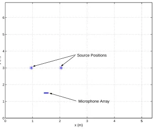
5.3.1 Experimental Setup . . . 82
5.3.2 Single Source . . . 84
5.3.3 Multiple Sources . . . 84
5.4 Conclusions . . . 87
6 Lower Bounds on the Mean Square Error (MSE) of an Estimator 89 6.1 Introduction . . . 89
6.2 Mean Square Error of an Estimator: an algebraic quantity . . . 92
6.3 Lower Bounds on the Mean Square Error (MSE) of an Estimator . . . 94
6.3.1 Derivation of the Barankin Bound . . . 96
6.4 Toward a Piecewise Approximation of the Barankin Bound . . . 98
6.4.1 An Alternative Look at Existing BB Approximations . . . 100
6.4.2 A New Practical BB Approximation . . . 101
6.4.3 General lower bounds expressions . . . 102
6.5 DOA Estimation Analysis . . . 103
6.5.1 General observation model . . . 103
6.6 Conclusions . . . 106
7 Conclusions 107 7.1 Summary and Conclusions . . . 107
7.2 Future Work . . . 110
A Appendix 111
List of Figures
2.1 Source in the far field emitting a signal received by the array of microphones. 9 2.2 The wavefronts arriving at a Uniform Linear Array (ULA) with
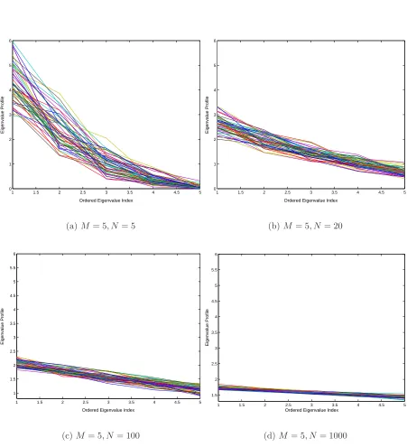
inter-microphone spacing ∆. . . 13 3.1 A Delay and Sum beamformer. . . 25 4.1 Profile of the ordered eigenvalues under the noise-only assumption for 50
independent trials, with M=5 and various values of N. . . 53 4.2 Profile of ordered noise eigenvalues in the presence of 2 sources, and 10
microphones. The ordered profile of the observed eigenvalue is seen to break from the noise eigenvalue distribution, when there are sources present. . . 54 4.3 Profile of ordered noise eigenvalues for several realizations. The circles
through the centre show the mean value for each eigenvalue. The distance between the upper and lower triangles is the spread of the eigenvalue and the chosen threshold is equal to half this distance. . . 57 4.4 Threshold computation for each step in the case where M = 5 and N = 10. 60 4.5 Results for the EFT, the MDL and the AIC. In this case the correct model
order is 2, the number of snapshotsN = 6, and the number of microphones
M = 5. The EFT thresholds have been determined to result in Pf a = 1% . 61
4.6 Results for the EFT, the MDL and the AIC. In this case the correct model order is 2, the number of samples N = 6, and the number of microphones
M = 5. The thresholds for the EFT have been determined to result in
Pf a = 10% . . . 62
4.7 Results for the EFT, the MDL and the AIC for simulated case of 2 speech sources received in presence of complex Gaussian White Noise and no re-verberation, for the case where N = 10 andM = 5. The thresholds for the EFT have been determined to result in Pf a = 10% . . . 63
LIST OF FIGURES x
4.9 Male source signals . . . 64 4.10 Female source signals . . . 65 4.11 Impulse responses from the sources to the centre microphone in the array.
These responses are found using EASET M acoustic simulation software.
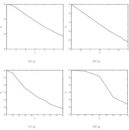
The impulse responses are simulated for a given setup based on the acous-tical properties of the venue and the geometrical configuration of the source and microphone array. . . 65 4.12 Probability of false alarm for the EFT, the MDL and the AIC using room
simulator EASE, as the Useful-to-Detrimental Ratio, U25, is increased. . . . 66
5.1 Performance of MUSIC, MLE and TDE techniques, for a speech signal arriving at an array of M = 5 microphones and window length N = 50 samples. Results are taken over 100 Monte Carlo trials for increasing SNR. 75 5.2 The normalised ML spatial spectrum for decreasing SNR (equation (5.1)).
The true DOA value is indicated by the arrow. . . 76 5.3 The normalised MUSIC spatial spectrum for decreasing SNR (equation
(5.8)). The true DOA value is indicated by the arrow. . . 77 5.4 The normalised TDE cross-correlation for decreasing SNR (equation (5.9)).
The true DOA value is indicated by the arrow. . . 78 5.5 Performance of MUSIC, MLE and TDE techniques, when 2 speech signals
arrive at an array of M = 5 microphones, and window length N = 50 samples. The results are averaged over 100 Monte Carlo trials for increasing SNR. . . 80 5.6 Results of MUSIC, MLE and TDE techniques, for estimating the DOA
of 2 white noise sources arriving at an array of M = 5 microphones, and window length N = 100 samples. The sources move toward each other in steps of 10o, and the results are averaged over 100 Monte Carlo trials at
each position. . . 81 5.7 Performance of MUSIC, MLE and TDE techniques, for the case of a single
speech signal arriving at an array of M = 5 microphones, with window length N = 50 samples. The DOA is equal to 70o and the results are
shown for increasing U25, with averages taken over 100 Monte Carlo trials. 82
5.8 Performance of MUSIC, MLE and TDE techniques, for two speech signals arriving at an array of M = 5 microphones, with window length N = 100 samples. The DOAs are equal to 70o and 110o, and the results shown here
are the average estimates taken over 100 Monte Carlo trials for increasing
LIST OF FIGURES xi
6.1 Three regions of operation observed for a non-linear estimator. . . 91 6.2 Comparison of MSE lower bounds versus SNR when estimating the DOA
List of Tables
4.1 Results found by EFT, AIC and MDL tests using experimental recordings of two different male speakers. . . 67 4.2 Results found by EFT, AIC and MDL tests using experimental recordings
of two different female speakers. . . 67 4.3 Results found by EFT, AIC and MDL tests using experimental recordings
of one male and one female speakers. . . 68 5.1 Results found by MUSIC, ML and TDE for experimental recordings of a
white noise source with DOA = 120o. The results are averaged over 100
Monte Carlo trials using a window length ofN = 100 samples. . . 85 5.2 Results found by MUSIC, ML and TDE for experimental recordings of 2
white noise sources with DOAs of 90o and 120o. The results are averaged
over 100 Monte Carlo trials using a window length ofN = 100 samples. . 86 5.3 Results found by MUSIC, ML and TDE for experimental recordings of 2
male speakers with DOAs of 70o and 110o. The results are averaged over
100 Monte Carlo trials using a window length of N = 100 samples. . . 87
List of Acronyms
DOA Direction Of Arrival
pdf Probability Density Function MSE Mean Square Error
ML Maximum Likelihood
MUSIC MUltiple SIgnal Classification TDE Time Delay Estimation
SNR Signal to Noise Ratio MSE Mean Square Error CRB Cram´er Rao Bound MSB McAulay Seidman Bound
BB Barankin Bound
HCRB Hammersley Chapman Robbins Bound
1
Introduction
1.1
Introduction
Array processing has been an active area of research for many years now, and originally array processing techniques were developed for military applications. However, the dra-matic increases in computing power which have taken place over the last number of years have led to the widespread use of Digital Signal Processing (DSP) devices in consumer electronics, for both business and entertainment purposes. The phenomenal growth of this industry has provided many new and challenging problems for signal processing re-searchers, as there is a constant demand for increased speed, accuracy and robustness, while reducing price and size.
In particular the area of acoustical array processing has become an active research topic. This interest can be attributed to the host of potential applications, for example: sonar applications; medical applications such as lithotripsy; non-destructive testing and human-computer interfacing; as well as a wide range of entertainment applications e.g. tracking of acoustical sources during theatrical performances and acoustical ambiance re-creation.
At its most basic, signal processing is concerned with transmission of a signal that contains some desired information, and manipulation of this signal in order to extract this
1.2. Array Processing 2
information. In array signal processing the signal or signals are emitted and/or received by an array. By array, we mean a set of receivers, that are spatially distributed. This separation of the receivers means that as well as the signal being temporally sampled, i.e. a value is received at each time instant, it is also spatially sampled as a value is received at each of the array elements. The advantage of using an array of receivers is this ability to exploit both the spatial and temporal characteristics of the signal.
Acoustical array processing is concerned with detection and manipulation of signals emitted by acoustical sources and has numerous applications in sonar, medicine, audio, active noise control etc. When dealing with acoustic sources the signals are received by an array of microphones.
1.2
Array Processing
For array signal processing purposes signals can be divided into two groups: those that have a fixed behaviour, called deterministic signals, and those that change randomly, called stochastic or random signals. Deterministic signals can be completely specified as a function of time and therefore the signal can be predicted from a number of previous time samples.
On the other hand stochastic or random signals cannot be easily characterised by a mathematical expression, and instead use must be made of prior knowledge and proba-bilities in order to analyse the signal behaviour, for example the use of a prior probability of a parameter to estimated the current value.
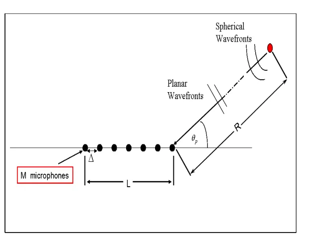
The signals of interest can be further classified as narrow- or wideband. A narrowband signal is one whose amplitude and phase vary slowly relative to the time taken for it to propagate across the array. A broadband signal is then a signal that is not narrowband, or a signal which has a relatively large frequency bandwidth compared to its centre frequency. The source emitting the signal can be classified as near-field or far-field. Near-field sources are located close enough to the array for the wavefront arriving at the array to be spherical. On the other hand, the wavefronts arriving from a far-field source have been propagating for long enough for the wavefronts to be planar, i.e in straight horizontal lines as they arrive at the array.
As the signal travels through the propagating medium it will be perturbed by additive noise and interfering signals. The presence of these signals change the properties of the received signal and make it difficult to extract the desired information.
1.2. Array Processing 3
white noise, that is noise with equal quantities of all frequencies, is often made. One reason for making such an assumption is that it greatly simplifies the mathematics involved in subsequent signal models. Fortunately, it is also a good approximation of the true noise present in many cases.
In some situations, however, the noise present may not contain all frequencies, and this noise is instead called coloured noise. In these situations, if the spectrum of the coloured noise is known, a whitening filter is usually applied to whiten the noise. Once this has been done, the characteristics of white noise can once again be exploited for any mathematical modelling. However, this requires access to the noise signal separate from the information signal and this is often not possible in practical situations.
Interference, on the other hand, will usually have similar characteristics to the desired source signal, and may be generated by a similar source, e.g. people speaking in the background when trying to extract a specific speech signal. Another type of interference is due to reverberation or multi-path, when the desired signal is reflected off surfaces within the propagation environment causing multiple delayed arrivals of the desired signal. The degradation of the desired signal by interference and reverberation is usually very difficult to deal with, as it becomes confused with the desired signal and therefore cannot be easily identified or removed.
Once the signal has been received by the array, the objectives of any subsequent pro-cessing steps can be categorised as either signal enhancement or field characterisation. Signal enhancement occurs when the spatial characteristics of the array are used to im-prove the SNR of the signal received. This can be done by steering the array so that it receives signals from a certain direction only, thereby ignoring signals arriving from other directions. This technique is called beamforming and in its simplest form is performed by delaying the signals received at each of the array elements, and then adding these delayed signals.
The delay applied corresponds to the time delay experienced by a signal originating from the desired location, as it propagates across the array. Signals originating from other locations will therefore be filtered out. This spatial filtering is very useful in situations where the interfering and noise signals overlap the desired signal spatially or temporally, making other types of filtering difficult.
Field characterisation is concerned with estimation of the spatial properties of the source or sources. Before the location of the sources can be found the first step must be to identify the number of sources present. This process can be called model order determination.
1.3. Thesis Organisation 4
stationary signals the localisation step involves estimation of the range, asimuth and elevation of the source. The number of parameters to be estimated is reduced for far-field sources, as only the asimuth and elevation can be estimated. These parameters are commonly further reduced by assuming the source and array are in the same plane, i.e. at the same height, which reduces the localisation problem to that of estimating the asimuth Direction of Arrival (DOA) of the signal only. In this thesis we are concerned with the estimation of the DOA of signals arriving from a far-field source. Extension to the situation where the source and array are not on the same plane, and the elevation must also be estimated is straight-forward.
Estimation of the DOA of an arriving signal has been an active area of research for many years now, and a vast number of algorithms and approaches exist. While many of these methods were developed originally for narrowband signals, they may also be applied to situations of broadband sources such as those encountered in acoustical array processing. In order to apply narrowband localisation techniques the signals are first broken down into narrowband bins, and localisation is then performed individually on each bin. These individual results are then combined to give an overall DOA estimate.
Despite the many localisation techniques that have been developed, the problem of DOA estimation continues to be a challenging problem. One of the difficulties lies in the fact that there is no guaranteed way of finding the best or optimal method of estimation for all situations. Instead sub-optimal methods must be used, and the most suitable approach is selected by taking into account characteristics of the source and environment. In order to determine the suitability of a proposed estimation method (i.e. the esti-mator) its performance can be compared to the best possible performance. This allows a decision to be reached on whether or not the estimator performance is satisfactory, or if it can be improved upon. It can also be determined whether or not it will ever be possible to achieve the required performance. One method of evaluating the best possible performance is by the use of lower bounds on the Mean Square Error (MSE) bounds, which provide a bound on the minimal MSE that can be achieved.
1.3
Thesis Organisation
1.3. Thesis Organisation 5
Density Function (pdf) and commonly applied assumptions. The selection of a suitable estimator and the criteria used to evaluate estimator performance are then considered. These criteria can then be applied in order to find the optimal estimator for a given esti-mation problem. However, it is shown that it is not always possible to find an expression for the optimal estimator, and that DOA estimation is an example of such a situation. We can therefore conclude that for this problem it is instead necessary to select a sub-optimal estimator that has desirable properties for the given situation. The commonly applied sub-optimal DOA estimators are then considered in chapter 3 and the main contributions to the area of DOA estimation are reviewed.
In chapter 4 the initial step in characterisation of the sources, that of model order determination is discussed. Acoustical model order determination presents a challenging problem due to both the wideband nature of the source and the fact that the amount of data available for a given source location may be limited. Classical methods operate well for determining the number of narrowband sources when large amounts of data are available. However, they are unreliable for the difficult situation considered here.
To this end, a method for determining the number of acoustical sources is proposed here. This method is based on the profile of the noise eigenvalues of the observed data correlation matrix as introduced by Grouffaud et al. [1]. This method is suited to the difficult operating scenarios encountered in acoustical source localisation. In particular this method is shown to out-perform classical detection methods for the situations where a small amount of data is available for a given source location.
This then leads to a study of three of the most well-known sub-optimal estimators, in chapter 5. The performance of these estimators is compared using both simulations and experimental recordings for a variety of source numbers and locations. The effects of interference and additive noise on the estimators is considered, allowing us to draw some conclusions on estimator behaviour, and the suitability of the estimators for different localisation problems.
In chapter 6 the best possible performance that can be achieved by an estimator for a given localisation problem is evaluated. This is done using lower bounds on the Mean Square Error (MSE), which provide a bound on the minimum MSE that can possibly be achieved.
1.4. Contributions 6
Conclusions are drawn in chapter 7 by commenting on the results from the previous chapters and finally, some proposals for future work are presented.
1.4
Contributions
The work done in the course of this thesis has led to the following papers:
1.4.1
Journal Papers:
1. A. Quinlan, J. P. Barbot, and P. Larzabal, “Automatic determination of the number of targets present when using the time reversal operator (TRO),” Journal Acoustical Society of America (JASA), vol.119, n.4, pp. 2220-2225, 2006.
2. A. Quinlan, J. P. Barbot, P. Larzabal, and M. Haardt, “Model order selection for short data: An exponential fitting test (EFT),” EURASIP JASP (European Journal Applied Signal Processing), Accepted for publication.
1.4.2
Conference Papers:
1. A.Quinlan and F. Boland, “Using the singer’s formant to reduce inaccuracies in the location of a singer on stage,” in Proc. Irish Signals and Systems Conference (ISSC), Belfast, Ireland, 2004.
2. A. Quinlan and F. Boland, “The effect of vibrato on singer localisation,” in Proc. GSPx Conference, Santa Clara, CA, 2004.
3. A. Quinlan, E. Chaumette, and P. Larzabal, “A direct method to generate approxi-mations of the Barankin bound,” in Proc. IEEE Int. Conf. Acoust., Speech, Signal Processing (ICASSP), Toulouse, France, 2006.
2
Estimation Using Array Processing
Techniques
2.1
Introduction
The use of array signal processing techniques for source localization has been an active area of research for many years, however it remains a challenging problem. The work presented in this thesis is concerned with localization of an acoustic source using an array of microphones. In this chapter the mathematical background of estimation is recalled. The terms defined here are then used throughout the thesis.
There are two possible approaches to the analysis of the data received by the micro-phone array: parametric and non-parametric. Parametric techniques assign a mathemat-ical model with a fixed number of parameters to the observed data, and the parameters of the model are selected so that the observations fit this model. These techniques use information that is known or assumed to be known about the observed data in order to determine a suitable model. The accuracy of the method is therefore reliant on the accuracy of the underlying model. In non-parametric techniques, on the other hand, no model is imposed on the data.
The work presented here focuses on parametric methods, in which the required
2.2. Modelling the Received Data 8
mation is expressed as a parameter of the received signal [2]. This parameter is then be estimated from the observations.
2.2
Modelling the Received Data
Firstly we consider the source, which can be classified as near-field or far-field depending on its distance from the array. If the source is in the near-field then the wavefronts reaching the array are spherical. For this type of source there is a vector of spatial parameters to be estimated containing both bearing and range information.
As the source is moved farther from the array the wavefronts become planar and parallel, as shown in figure 2.1. A source is considered to be in the far-field if:
R > 2L
2
λ , (2.1)
where R is the distance from the source to the array, L is the length of the array, and
λ is the wavelength of the arriving wave. When the source is in the far-field only the bearing information, or Direction of Arrival (DOA), can be used to characterise the source spatially [3]. This is the situation being investigated in this thesis. A common assumption is that the source and array are in the same plane, thereby further reducing the spatial parameters to be estimated, and the wavefronts arriving at consecutive microphones differ only by an amplitude coefficient and a time-delay.
The scenario where there are P far-field sources present, and the emitted signals are received by an arbitrary array ofM microphones is now considered. The impulse response of the mth microphone to a signal sp(t), emitted from thepth source is denoted hpm(t).
This impulse response depends on the locations of both the source and the microphone, the propagating medium, and any gain or attenuation introduced by the microphone itself. The time delay of the pth signal arriving at the mth microphone is denoted τpm. The
output at the mthmicrophone can then be written as:
xm(t) = P
X
p=1
hpm(t)∗sp(t−τpm) +nm(t), (2.2)
where (∗) denotes convolution and nm(t) is the additive noise signal received by the mth
microphone, it is assumed that nm(t) is independent of sp(t), and that P < M. The
2.3. Complex Signal Representation 9
Figure 2.1: Source in the far field emitting a signal received by the array of microphones.
x(t) =
x1(t)
x2(t)
...
xM(t)
= PP
p=1hp1(t)∗sp(t−τp1)
PP
p=1hp2(t)∗sp(t−τp2)
...
PP
p=1hpM(t)∗sp(t−τpM)
+
n1(t)
n2(t)
...
nM(t)
. (2.3)
2.3
Complex Signal Representation
In array signal processing the complex representation of a signal is often used. This representation is based on the assumption that the signal is narrowband. In many cases this narrowband assumption does not hold, and in these situations the bandwidth of the signal must be divided into smaller frequency bins so that the narrowband assumption will hold across each frequency bin, and the following analysis will then hold for each bin. The emitted signal sp(t) can be expressed in terms of a modulated centre frequency
ω:
sp(t) =αp(t) cos
ωt+φp(t)
. (2.4)
2.3. Complex Signal Representation 10
αp(t−τp) ≈ αp(t), (2.5)
φp(t−τp) ≈ φp(t), (2.6)
which implies that:
sp(t−τp) = αp(t−τp) cos
ω(t−τp) +φp(t−τp)
(2.7)
≈ αp(t) cosωt−ωτp +φp(t). (2.8)
The time-delay can now be modelled as a phase-shift of the carrier frequency. Following from the assumption that the signal is narrowband, the impulse response can be taken to be constant across the frequency band of interest. The stationary response of the mth
microphone to the signal sp(t) can therefore be expressed as:
rpm(t) = hpm(t)∗sp(t−τpm) (2.9)
= hpm(t)∗αp(t) cos
ωt−ωτpm+φp(t)
(2.10) = Hpm(ω)αp(t) cos
ωt−ωτpm+φp(t)
, (2.11)
where Hpm(ω) is the Fourier transform of the impulse response hpm(t). Expressing
Hpm(ω) in terms of its phase, argHpm(ω), and magnitude, |Hpm(ω)|, and letting βpm =
|Hpm(ω)|, (2.11) can be re-written as:
rpm(t)⋍βpm(ω)αp(t) cos
ωt−ωτpm+φp(t) + argHpm(ω)
, (2.12) Using a complex signal representation of the received signal, the time-delay can then be expressed as a multiplication by a complex number. Considering the case where there is no noise present, the complex representation of the signal received by themthmicrophone is given by:
rpm(t) = xim(t) +jxqm(t) (2.13)
= βpm(ω)e− jωτpmα
p(t)ejφp(t) (2.14)
= βpm(ω)e−jωτpmse
p(t), (2.15)
where sep(t) is the complex envelope of the signal sp(t), and sep(t) = αp(t)ejφp(t). Then,
2.4. Parametric Signal Model 11
a(θp) =
βp1(ω)e−jωτp1
βp2(ω)e−jωτp2
...
βpM(ω)e−jωτpM
. (2.16)
This complex vector describes the response of each microphone, including geometric path differences, to a signal arriving at an angle ofθp. Throughout the thesis this vector is
called the array response vector, however it can also be referred to as the steering vector, the location vector or the transfer function vector.
The in-phase and quadrature components of xm(t), xim(t) and xqm(t) respectively, are
given by:
xim(t) = |Hpm(ω)|αp(t) cos
φp(t) + argHpm(ω)−ωτpm
(2.17)
xq
m(t) = |Hpm(ω)|αp(t) sin
φp(t) + argHpm(ω)−ωτpm
. (2.18)
2.4
Parametric Signal Model
The required parameter for each source is the Direction of Arrival (DOA), θp, and the
DOA associated with the each of the P sources present must be estimated from the data received by the array. In the case considered here the angle of elevation is assumed to be zero, as the microphones and source are assumed to be the same height. However, the results derived here can easily be extended to the general case, where both bearing and elevation are unknown.
From equations (2.3) and (2.15), the parameterised data model for the pth source is given by:
x(t) =
x1(t)
x2(t)
...
xM(t)
= P X p=1
a1(θp)
a2(θp)
...
aM (θp)
s˜p(t) +
n1(t)
n2(t)
...
nM (t)
(2.19) = P X p=1
a(θp) ˜sp(t) +n(t). (2.20)
2.4. Parametric Signal Model 12
x(t) = [a(θ1),a(θ2), . . . ,a(θP)] [es1(t), . . . ,esP(t)] T
+n(t). (2.21) Then defining theM ×P matrix A(θ) the columns of which are given by the array response vectors associated with each of theP sources, equation (2.21) can be re-expressed as:
x(t) =A(θ)se(t) +n(t), (2.22) with: θ = θ1 θ2 .. . θP
. (2.23)
This model is applicable to an array of arbitrarily located microphones assuming that the sources are located in the far-field; thatP < M; and that the sources are non-coherent, where two signals are coherent if one is a scaled and delayed version of the other [2]. A Uniform Linear Array (ULA) is commonly used as it leads to simplification of the data model. This is the array configuration considered here. However, the results found are easily extended to other array configurations.
For a ULA with an inter-microphone spacing ∆, τpm can be related to the DOA by
the following expression, as seen in figure (2.2):
cos (θp) =
vτpm
∆ , (2.24)
where v is the speed of sound as it travels through air. Due to the far-field conditions it can be assumed that βpm is constant for m = 1, . . . , M, and ∀p = 1, . . . , P.. Then,
substituting for τpm in equation (2.16), the array response vector can now be expressed
as:
a(θp) =a1(θp)
1
e−jω2∆cosv(θp)
.. .
e−j(M)ω∆cosv(θp)
. (2.25)
2.4. Parametric Signal Model 13
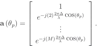
Figure 2.2: The wavefronts arriving at a Uniform Linear Array (ULA) with inter-microphone spacing ∆.
a(θp) =
1
e−j(2)2π∆
λ cos(θp)
...
e−j(M)2πλ∆cos(θp)
. (2.26)
If ∆ > λ
2 then spatial aliasing can occur, i.e. there exists θ1, θ2 ∈ [0, π] such that for
θ1 6=θ2:
e−j2πλ∆cos(θ1) =e−j2πλ∆cos(θ2). (2.27)
Therefore, in order to avoid this problem, the array must be designed so that: ∆≤ λmin
2 , (2.28)
2.5. Probability Density Function (pdf) of the Observed Data 14
2.5
Probability Density Function (pdf ) of the
Ob-served Data
Due to the random nature of the observation vector the probability of correctly deter-mining the required parameters will never be equal to 1. Instead the observed data can be characterised by the Probability Density Function (pdf) denoted fθ(x). As the pdf is
dependent onθ there is a different pdf associated with each different realisation ofθ. The accuracy of the estimator is directly linked to that of the pdf, the correct choice of pdf will therefore greatly influence the performance of the estimator.
Estimation based solely on the pdf of the observed data is called classical estimation [4]. This is the estimation problem considered here and it is assumed throughout that no prior information about the parameters is available. Alternatively Bayesian estimation can be used if prior knowledge of the parameter values exists [4]. In this situation the parameter to be estimated is viewed as a realization of the random variable θ.
In this work deterministic estimation is considered, and for the sake of simplicity the case of estimating a single, i.e. P = 1, real, deterministic parameter is considered initially. These results are then extended to include estimation of multiple deterministic parameters.
In certain situations it may be more convenient to estimate a function of the required parameter rather than the parameter itself. Therefore in the following the general case of estimating a function g(θ) is considered, where g(θ) may or may not be equal to
θ. Correspondingly the estimator used to estimate the parameter value based on the observations is denoted gd(θ) (x).
For many practical estimation problems the pdf will not be known and must instead be approximated. A random variable xis said to be Gaussian, with distribution N(mx, σx)
if its pdf has a Normal distribution. Assuming a Gaussian distribution, and lettingP = 1 the pdf of the received data, as given in equation (2.21), is expressed as:
fθ(x) =
1
σx
√
2πe
−12k
x−mx
σx k
2
, (2.29)
wheremx=E[x], and σ2x is the variance of [x].
2.6. Estimator Performance Evaluation 15
If x1, x2, . . . , xN are a set of independent random variables, with mean m and finite
variance σ2, then:
x1+. . .+xn+. . .+xN
N −−−−−−−−−−−−−−−−−−−−−→converges to distributionN
→∞
N E[x],
r
σ2 x
N
!
, (2.30)
Therefore if we have N independent observations of the same random experiment,
x1, x2, . . . , xN, for sufficiently large N the estimator N1 P dg(θ) (x) will have a Gaussian
distribution:
N
Ehgd(θ) (x)i,
s
σ2
d
g(θ)
N
, (2.31)
where σ2
d
g(θ) is the variance of the estimatorgd(θ). We now need to find an estimator that
will assign an estimate to each set of observations x= [x[1], x[2], . . . x[N]]. The quality of such an estimator must be quantified in order to see if it meets requirements, and ideally we wish to find the optimal estimator for a given situation. This naturally leads to the question of what measurements are needed to evaluate the estimator performance, and what criteria should be met in order for an estimator to be considered “optimal”.
2.6
Estimator Performance Evaluation
When evaluating the performance of an estimator the basic question that must be ad-dressed is “How accurate are the results provided by this estimator?”, or put another way, “How close will the resulting estimates be to the true values?”. The aim then is to select the best possible estimator, but in order to do this the term “best” must be quantified.
The first factor to be considered is whether or not the mean or expected value of the estimator is equal to the true parameter value, i.e. is:
Ehgd(θ) (x)i=g(θ). (2.32) If this is true, then the estimator is said to be unbiased. If this is not the case, then the estimator is biased, with bias given by:
2.7. Finding the Optimal Estimator 16
The effects of such an error therefore cannot be removed by averaging. While an unbi-ased estimator is not necessarily a good estimator, a biunbi-ased estimator is generally highly undesirable [4].
The second measurement used to characterize the estimator performance is the vari-ance, which measures the dispersion of the estimates around their expected value:
V argd(θ) (x)=Egd(θ) (x)−Ehgd(θ) (x)i2
. (2.34)
Clearly the more accurate the estimator, the smaller the variance will be [4].
The Mean Square Error (MSE) is commonly used as a measurement of the quality or precision of an estimator. Defining Ω as the observation space, the MSE can be expressed as:
MSEhgd(θ) (x)i = Egd(θ) (x)−g(θ)2
(2.35) =
Z
Ω
d
g(θ) (x)−g(θ)2fθ(x)dx (2.36)
= dg(θ)−g(θ)2
θ. (2.37)
From equation (2.35) we can see that the MSE can also be expressed as:
MSEhgd(θ) (x)i=V arhgd(θ) (x)i+Bias2hgd(θ) (x)i. (2.38)
Then for an unbiased estimator:
Biasgd(θ) (x) = Ehgd(θ) (x)i−g(θ) = 0, (2.39) =⇒ MSEgd(θ) (x)=V argd(θ) (x). (2.40) A final consideration when evaluating the performance of an estimator is the com-plexity of the computations involved. While an estimator may provide highly accurate results, it will be of little practical use if it cannot be quickly and easily implemented. In such situations, an estimator with lower accuracy may in fact be preferable, particularly if real-time estimation of the parameters is necessary.
2.7
Finding the Optimal Estimator
2.7. Finding the Optimal Estimator 17
estimator to be realisable if its definition does not rely on unknown or unobservable quantities. There are however certain approaches that will, in some cases, produce a closed form expression for such an estimator. The most well known of these approaches are discussed here.
Using the MSE as a measurement of the estimator quality, we aim to find a realizable estimator with the minimum MSE. The following questions therefore arise “does such an estimator exist?” and if so, “how can such an estimator be found?”.
In the following the general case of estimating a vector of unknown parameters is considered.
2.7.1
Minimum Mean Square Error (MMSE) Estimator
One approach [6] is to minimize the expression for the overall weighted MSE and find the estimator that achieves this, i.e the aim is to find the optimal estimator for all values of
theta, called the optimal global estimator gd(θ) (x)globopt ,with the minimum MSE. The expression for the weighted MSE is given by [6]:
MSEhgd(θ) (x), ∂i =
Z
Θ
MSEhgd(θ) (x)i∂(θ)dθ (2.41) =
Z
Θ
Z
Ω
d
g(θ) (x)−g(θ)2fθ(x)∂(θ)dxdθ, (2.42)
where∂(θ) is a strictly positive weighting function defined over Θ, such thatRΘ∂(θ)dθ=1.
The weighted MSE is introduced here in order to express the minimization in a form sim-ilar to that of risk minimization in Bayesian estimation, allowing exploitation of results previously established in this area [7]. From equation (2.41) it can be seen that in this case∂(θ) is equivalent to the prior in Bayesian estimation theory. TheMSEhgd(θ) (x), ∂i
can be re-expressed in certain cases as:
MSEhgd(θ) (x), ∂i =
Z
Ω
Z
Θ
d
g(θ) (x)−g(θ)2∂(θ)fθ(x)dθdx. (2.43)
Minimization of the MSE is therefore equivalent to minimization of the inner integral:
Z
Θ
d
g(θ) (x)∂(θ)fθ(x)dθ−
Z
Θ
g(θ)∂(θ)fθ(x)dθ = 0, (2.44)
Then setting:
d
2.7. Finding the Optimal Estimator 18
this gives:
d
g(θ) (x)globopt =
R
ΘRg(θ)∂(θ)fθ(x)dθ Θ∂(θ)fθ(x)dθ
, (2.46)
where gd(θ) (x) is a realisable estimator as it is independent of theta. Unfortunately however, calculation of this estimator is often impossible and there is no known method for determining a suitable ∂(θ), that will lead to the minimum MSE for allθ ∈Θ [4].
As the strategy of minimizing the overall or global MSE does not necessarily pro-duce a computable expression for the minimum MSE estimator, the MSE is minimized instead for a given parameter valueθ, in order to find a realizablegd(θ) (x)locopt, that is non-trivial gd(θ) (x)optloc 6=g(θ).While this approach is simpler than the global approach, as
d
g(θ) (x)locopt is based on local optimization it is unlikely to produce a realizable estimator that is not “clairvoyant” i.e. that does not depend on the unknown parameter value [6]. Minimization of the local MSE under non-bias constraints is discussed in detail in chap-ter 6, when it is used for the calculation of the best possible performance of an estimator using minimal performance bounds. It can therefore be concluded that the procedure of minimizing the MSE is unlikely to produce a realizable estimator, and an alternative strategy must be adopted.
2.7.2
Minimum Variance Unbiased (MVU) Estimator
An alternative approach is to search for the unbiased estimator with the minimum variance for all possible values ofθ. This Minimum Variance Unbiased (MVU) estimator does not always exist, as it is common for different estimators to have minimum variance depending on the value of θ.
The minimum possible variance that can be attained by an unbiased estimator is characterised by the Cramer-Rao Bound (CRB) [8]. Therefore, if an estimator exists whose variance equals the CRB for each value of θ, this must be the MVU, and taking variance as a measure of optimality, the CRB can then be used to find an expression for the optimal estimator. Any estimator that has variance equal to the CRB is called an efficient estimator.
In order to derive the CRB, the following regularity condition is assumed to be met:
E
∂lnfθ(x)
∂θ
2.7. Finding the Optimal Estimator 19
and an efficient estimator exists if (and only if) the following factorization can be made:
∂lnfθ(x)
∂θ =F(θ) (h(x)−g(θ)), (2.48)
where gd(θ)M V U (x) =h(x).
The variance of an efficient estimator is equal to the Cramer Rao Bound (CRB) and can be expressed as follows (see chapter 6 for a full discussion on the derivation of the minimal variance of an estimator and estimator performance bounds.)
Cd
g(θ)M V U(x) ≥ −E
∂2lnf
θ(x)
∂θ∂θT
−1
. (2.49)
When a linear model can be used to describe the data this approach yields a closed form expression for the MVU estimator, and its variance is equal to the CRB. Using the classical general linear model [4], the observed data can be described as:
x=Hθ+n (2.50)
where xis the (N ×1) observation vector andHis the known (N ×P) transfer function matrix. In this case, H is a linear function of the (P ×1) vector of unknown parameters
θ = [θ1, θ2, . . . , θP] T
, and n is the (N ×1) noise vector with pdf N(0,C). The pdf of x
is:
fθ(x) =
1 (2π)N2 √detC
exp
−1
2(x−Hθ)
T
C−1(x−Hθ)
, (2.51)
and so:
∂lnfθ(x)
∂θ = H
T
C−1H dg(θ) (x)−g(θ), (2.52) resulting in the efficient and MVU estimator, which is the weighted Least Squares (LS) estimate:
d
g(θ)M V U(x) = HTC−1H−1HTC−1x, (2.53)
with variance:
2.7. Finding the Optimal Estimator 20
However, in many situations it will not be appropriate to use a linear model to describe the data, as arises when estimating the Direction of Arrival (DOA) of a source signal. This situation is now considered, using the data model defined in equation (2.22) where in this case nis White Gaussian Noise (WGN) with varianceσ2.The pdf of the observed data is given by:
fθ(x) =
1 (2πσ2)N2
exp
− 1
2σ2 (x−A(θ)s)
T
(x−A(θ)s)
, (2.55)
leading to:
∂lnfθ(x)
∂θ =
s
2σ2
(
∂A(θ)
∂θ
T
(x−A(θ)s) + (x−A(θ)s)T
∂A(θ)
∂θ
)
, (2.56)
where:
∂A(θ)
∂θ =
∂A(θ1)
∂θ ∂A(θ2)
∂θ
...
∂A(θP)
∂θ (2.57)
In this situation, factorisation as shown in equation (2.48) in order to find an expres-sion for the MVU estimator is not possible. In fact, for non-linear data models efficient estimators will only be found under asymptotic conditions (high SNR [9] and/or large number of snapshots [8]). This is due to the fact that asymptotically the pdf becomes more concentrated around the true parameter value θ, causing the estimates to lie in a smaller interval aboutθ. In this case the estimator is said to be consistent. The relation-ship is approximately linear in this region and observations rarely occur in the non-linear region, resulting in asymptotic efficiency. (For a detailed discussion on the performance of non-linear estimators, see chapter 6). Therefore unless operating under asymptotic conditions it will not be possible to find an efficient estimator for DOA estimation.
2.8. Conclusion 21
that a minimal sufficient statistic is just as informative as the original data, but it can be computed from any other sufficient statistic; no further compression of the data is possible, without losing some information. If a sufficient statistic is found, then the MVU estimator must be a function of this statistic.
Using the Neyman-Fisher factorization a sufficient statistic can be found directly from the pdf, which is assumed to be known [4]:
fθ(x) =f(T(x),θ)h(x), (2.58)
where if θ is a p−dimensional vector, then the statistic T(x) is a p−dimensional function, f is a function depending only on T and θ, and h is a function depending only on the observations x. The difficulty however, arises in situations where this factorization is not obvious, and in these cases it is possible that a sufficient statistic, other than the observed data itself, does not exist.
If a sufficient statistic does exist, the Rao-Blackwell-Lehmann-Scheffe (RBLS) the-orem can be applied in order to determine the corresponding estimator. Firstly, a
p−dimensional function f must be found such that:
E[f(T)] =θ. (2.59) Then if f(T) is the only unbiased function of the sufficient statistic, the statistic is said to be complete, and the MVU estimator is given by:
d
g(θ) (x) = f(T) . (2.60) This approach can be seen to provide a means of finding an expression for the MVU estimator provided a minimal sufficient statistic exists. However, even in situations where such a statistic does exist, verification of its completeness can be very difficult.
It can therefore be seen that there is no guaranteed way to find an expression for an optimal estimator for the non-linear data models being considered here, and even if such an estimator exists it is not guaranteed to be realisable, as it may require knowledge of unknown parameters. Sub-optimal estimators must instead be considered in order to select a suitable estimator for the given estimation problem.
2.8
Conclusion
2.8. Conclusion 22
discussed. The use of the pdf of the data to estimate the desired parameters was then considered, and the criteria that can be used for estimator evaluation were developed and used to define an “optimal estimator”.
The optimality criterion initially selected was the minimal MSE, however it was shown that minimization of the MSE does not provide an expression for an optimal estimator. The next optimality criterion considered was the variance, and it was seen that for some estimation problems the CRB can be used to find a direct expression for an efficient estimator, which is also the MVU estimator. However, for non-linear estimation problems such as DOA estimation, it is not possible to find an efficient estimator. The fact that no efficient estimator exists does not exclude the possibility that an MVU estimator exists, and use can be made of sufficient statistics in order to determine the MVU estimator in such a situation. However, determining the sufficient statistic involves factorization of the pdf, which may not be obvious, and in many cases a minimal sufficient statistic does not exist. Even if a minimal sufficient statistic is found, it must be checked for completeness in order to result in an expression for the MVU estimator, and verification of the completeness can be extremely difficult.
3
Direction of Arrival (DOA) Estimation
3.1
Acoustic Source Localization
Using a common problem specification, this chapter provides a unified explanation of classical Direction of Arrival (DOA) estimation techniques. Moreover, the classical signal processing techniques, which in many cases were developed for narrowband signal process-ing, are treated in the context of localization of broadband sources. Recent developments in the application of these classical techniques to acoustical array localisation are also discussed.
3.2
Beamforming
The earliest development of spatial filtering or beamforming dates back to the Second World War, when the conventional beamformer was developed. The aim of this beam-former was to enhance the received signal by “steering” the array in the direction of the desired source. This beamformer is simply an application of Fourier-based spectral analysis to spatio-temporally sampled data [2, 10, 11].
The ability of the beamformer to enhance signals from a desired direction can also be applied to the problem of DOA estimation. The output of the antenna is steered
3.2. Beamforming 24
in each possible direction of interest, and the power of the array output is measured for each direction. The values of θ, resulting in the maximum array output power are then chosen as the DOA estimates. Narrowband beamformers assume that the incident signal has a narrow bandwidth, centred at a particular frequency. If the incident signal is broadband then it can be divided into narrow frequency bands, and a weighted average of the DOA estimates found for each of these bands is then found (see section 3.3.1 for further discussion on these techniques).
Using the data model introduced in the previous chapter the signal received by the array at time t is given by:
x(t) =A(θ)se(t) +n(t), (3.1) where n(t) is assumed to Gaussian noise. The steered output of the array is found by linearly combining the spatially sampled data received at each sensor, and can be expressed as:
y(t) =wHx(t), (3.2)
where w is the complex weighting vector, and acts as a spatial filter applied to the signal which results in one particular direction being emphasized. For the case where N
snapshots of the signal are available the output power of the array is given by:
P (θ) = 1
N
N
X
t=1
|y(t)|2 (3.3)
= 1
N
N
X
t=1
wHx(t)xH(t)w (3.4)
= wHRwb , (3.5)
whereRb is the estimate of the spatial correlation matrix of the signal x(t):
b
R= 1
N
N
X
t=1
x(t)xH(t) (3.6)
The estimate of the DOA, bθ, is then given by:
b
θ = arg max
θ {P(θ)} (3.7)
3.2. Beamforming 25
As suggested by the name, the weights in a data independent beamformer are independent of the observations, and are chosen to produce a specified response regardless of the data received. On the other hand, the weights in a statistically optimum beamformer are chosen to optimize the array response, based on the statistics of the array data.
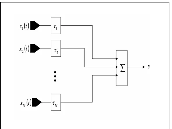
[image:40.595.167.465.231.455.2]3.2.1
Delay and Sum Beamformer
Figure 3.1: A Delay and Sum beamformer.
The Delay and Sum Beamformer (DSB) [10] is data independent, as it depends on the array geometry not on the received signal, and it is the simplest type of beamformer. Firstly the delay corresponding to a signal arriving from the directionθp is calculated for
each of the microphones in the array, and the signal received by each of the microphones is then weighted by the appropriate delay. This results in constructive re-enforcement of the signal arriving from the direction θp while signals arriving from other directions are
3.2. Beamforming 26
y(t) =
M
X
m=1
xm(t+τpm(θ)), (3.8)
P (θ) = 1
N
N
X
t=1
|y(t)|2 (3.9)
= 1
N
N
X
t=1
M
X
m=1
xm(t+τpm)
2
, (3.10)
whereτpm(θ) is defined in chapter 2 - section 2.2. The DOA estimates are then found by
searching for the P maxima ofP (θ).
An advantage of this beamforming approach is that it can be applied directly to broadband signals. However, the degree of resolution that can be achieved is strictly limited by the temporal sampling frequency of the data as delay differences less than the sampling rate cannot be resolved. Therefore in order to achieve higher resolution the sampling frequency must be increased resulting in an increased need for storage space and processing power.
3.2.2
Frequency Domain Beamforming
In order to increase the resolution that can be achieved without a corresponding increase in the sampling frequency required, beamforming can instead be performed in the fre-quency domain. Frefre-quency domain beamforming is inherently narrowband, and therefore broadband signals are divided into narrowband frequency bins centered onfc:
X(fc) =A(fc,θ)S(fc) +N(fc). (3.11)
Assuming once again that the array is a ULA, the array response function A(fc,θ)
is a function of the incident angle only, and represents the response of the array to
P complex exponentials at frequency fc, which arrive at the array with angles of θ =
[θ1,θ2,...,θp]. The frequency domain representation of the steered output of the array is
found by linear combination of these frequency components after applying the appropriate complex weights:
Y (fc) =WHX(fc). (3.12)
3.2. Beamforming 27
all other directions are attenuated. The output Power Spectral Density (PSD) is given by:
ΦY Y (fc) = Y (fc)Y∗(fc) (3.13)
= WH(f
c)RbXXW(fc), (3.14)
whereRbXX is defined in 3.6. The DOA estimates are then found for each frequency band
b
θ(fc) by selecting theP maxima of the output PSD:
b
θ(fc) = arg max
θ {ΦY Y (fc)} (3.15)
In order to produce a non-trivial solution of equation (3.7) the weight vector is chosen so that |W|= 1, resulting in the following weight vector for a given directionθ at a given frequency:
W(fc, θ) =
A(fc, θ)
p
AH(f
c, θ)A(fc, θ)
. (3.16)
Substitution of equation (3.16) into equation (3.14) produces the classical spatial spec-trum:
ΦBF (fc) =
AH(f
c, θ)R[XXA(fc, θ) AH(f
c, θ)A(fc, θ)
. (3.17)
The conventional beamformer is an extension of the classical Fourier based spectral analysis, and if the array in question is a ULA, then the resulting spatial spectrum in (3.17) can be viewed as a spatial domain version of the classical time-series domain periodogram. This similarity between the conventional beamformer and the time-series periodogram also extends to the resolution threshold experienced in the periodogram, and the maximum resolution that can be achieved for a ULA of M elements is:
∆ =
2π M
rads. (3.18)
3.2.3
Beamforming and Acoustical Source Localization
3.3. Subspace-Based Techniques 28
may perform poorly when applied to the reverberant situations encountered in acoustical source localization.
Several researchers have shown that the degradation of performance due to such effects can be reduced by the use of any a priori information that may be available. In [13] the nature (e.g. statistical non-stationarity, method of production, pitch, voicing, formant structure, and source radiator model) of the speech signal being localized is modelled by the “Dual Excitation Model”, providing a specific parameterization model which improves upon the general spatial filtering approach. Information on the nature of the speech signal is also used in [14] to distinguish between real sources and virtual sources arising due to reverberation. A priori knowledge has also been used to reduce the computational load of beamformer localization. In [15] the fact that the characteristic wavelengths of speech are comparable to the dimensions of the space being searched is exploited, allowing for the implementation of a coarse-to-fine search criterion in both the spatial and frequency domain.
In [16] a beamformer-based source localization technique within a particle filtering framework is proposed. The use of particle filters avoids the need for a comprehensive search of the source location space, and therefore allows for a computationally efficient beamforming scheme.
The similarity between the DSB and a Bayesian formulation was recently demonstrated in [17]. It was shown that when considered from the point of view of maximizing the likelihood the Bayesian formulation and Beamforming have been shown to be equal except for an energy term weighting which will not effect the likelihood of localizing a stationary signal, making the two methods identical in this case [17].
3.3
Subspace-Based Techniques
Subspace based DOA estimation methods exploit the geometrical properties of the cor-relation matrix of the received signals. A narrowband signal model is assumed as the signal subspace will differ for the different frequency bands in a broadband signal [18, 19]. Broadband incident signals are therefore transformed into the frequency domain, and di-vided into narrowband frequency bins as described in the previous section. Operating in the frequency domain, and assuming spatially white, zero-mean Gaussian noise, the correlation matrix of the observed signal is given by:
R(fc) = E
X(fc)XH(fc) (3.19)
3.3. Subspace-Based Techniques 29
where:
Rs(fc) =E
S(fc)SH(fc) , (3.21)
and Rs is assumed to be full rank. Once the matrix A(fc,θ) has full rank and
assum-ing P < M, the matrix A(fc,θ)Rs(fc)AH (fc,θ) has rankP, where P is the number of
sources present. Furthermore, every vector in the range space ofA(fc,θ)Rs(fc)AH(fc,θ)
is an eigenvector of R, associated with eigenvalue λ. Consequently, using the eigende-composition of the matrix, R can be re-expressed as:
R=
M
X
m=1
λmemeH
m. (3.22)
Arranging the eigenvectors in order of the decreasing size of their associated eigenval-ues, the signal and noise eigenvectors can then be separated:
R= PPm=1λmemeH m +
PM
m=P+1λmeme
H
m (3.23)
=EsΛsEH
s +σ2EnEHn, (3.24)
whereEsandEnare matrices containing respectively the signal and noise eigenvectors:
Es = [e1, . . . ,eP] (3.25)
En = [eP+1, . . . ,eM], (3.26)
and Λs =diag[λ1, . . . λP] are the eigenvalues associated with the signal eigenvectors.
Any vector orthogonal toA(fc,θ) is an eigenvector ofRassociated with an eigenvalue
σ2 [2]. Therefore En is orthogonal to A(f
c,θ)Rs(fc)AH(fc,θ),
and as A(fc,θ)Rs(fc)AH(fc,θ) is full rank, it follows that [2]:
R{Es} = R{A(fc,θ)} (3.27)
R{En} = R{Es}⊥=R{A(fc,θ)}⊥ =NAH(f
c,θ) (3.28)
whereR{Es}is the subspace spanned by the range ofEs, and NAH(f
c,θ) is the
null-space of AH(f
c,θ). Therefore, if the signal subspace is the subspace spanned by Es, and
the noise subspace is the subspace spanned by En, then we can see that the signal and noise subspaces are orthogonal to each other. This relation is the basis for all subspace based estimation techniques.
In practice the matrixR(fc) is unknown, and must be estimated from the observations:
b
R(fc) =
1
N
N
X
t=1