CodeX: Combining an SVM Classifier and Character N-gram Language
Models for Sentiment Analysis on Twitter Text
Qi Han, Junfei Guo
and
Hinrich Sch ¨utze
Institute for Nature Language Processing
University of Stuttgart
Stuttgart, Germany
{
hanqi, guojf
}
@ims.uni-stuttgart.de
Abstract
This paper briefly reports our system for the SemEval-2013 Task 2: sentiment analysis in Twitter. We first used an SVM classifier with a wide range of features, including bag of word features (unigram, bigram), POS fea-tures, stylistic feafea-tures, readability scores and other statistics of the tweet being analyzed, domain names, abbreviations, emoticons in the Twitter text. Then we investigated the ef-fectiveness of these features. We also used character n-gram language models to address the problem of high lexical variation in Twit-ter text and combined the two approaches to obtain the final results. Our system is robust and achieves good performance on the Twitter test data as well as the SMS test data.
1
Introduction
The challenge of the SemEval-2013 Task 2 (Task B) is the “Message Polarity Classification” (Wilson et al., 2013). Specifically, the task was to classify whether a given message has positive, negative or neutral sentiment; for messages conveying both pos-itive and negative sentiment, whichever is stronger should be chosen.
In recent years, text messaging and microblog-ging such as tweeting has gained its popularity. Since these short messages are often used not only to discuss facts but also to share opinions and sen-timents, sentiment analysis on this type of data has lately become interesting. However, some features of this type of data make natural language process-ing challengprocess-ing. For example, the messages are
usu-ally short and the language used can be very in-formal, with misspellings, creative spellings, slang, URLs and special abbreviations. Some research has already been done attempting to address these prob-lems, to enable sentiment analysis on this type of data, in particular on Twitter data, and even to use the outcome of sentiment analysis to make predic-tions (Jansen et al., 2009; Barbosa and Feng, 2010; Bifet and Frank, 2010; Davidov et al., 2010; Jiang et al., 2011; Pak and Paroubek, 2010; Saif et al., 2012; Tumasjan et al., 2010).
As the research mentioned above, our system used a machine learning based approach for sentiment analysis. Our system combines results from an SVM classifier using a wide range of features as well as votes derived from character n-gram language mod-els to do the final prediction.
The rest of this paper is organized as follows. Sec-tion 2 describes the features used for the SVM clas-sifier. Section 3 describes how the votes from char-acter n-gram language models were derived. Section 4 describes the details of our method. And finally section 5 presents the results.
2
Features
We pre-processed the tweets as follows: i) tok-enized the tweets using a tokenizer suitable for Twit-ter data, which, for example, recognize emoticons and hashtags; ii) replaced all URLs with the token
twitterurl; iii) replaced all Twitter usernames with the token @twitterusername; iv) converted all to-kens into lower case; v) replaced all sequences of repeated characters by three characters, for example, convertgoooooodtogoood, this way we recognize
the emphasized usage of the word; vi) expanded ab-breviations with a dictionary,1 which we will refer to asnoslang dictionary; vii) appended neg to all words from one position before a negation word to the next punctuation mark.
We represented each given tweet using 6 feature families:
• Lexical features(UG, BG): Number of times each unigram appears in the tweet (UG); num-ber of times each bigram appears in the tweet (BG).
• POS features (POS U, POS B): Number of times each POS appears in the tweet divided by number of tokens of that tweet (POS U); num-ber of times each POS bigram appears in the tweet (POS B). To tag the tweet we used the
ark-twitter-nlp tagger.2
• Statistical features(STAT): Various readabil-ity scores (ARI, Flesch Reading Ease, RIX, LIX, Coleman Liau Index, SMOG Index, Gun-ning Fog Index, Flesch-Kincaid Grade Level) of the tweet; some simple statistics of the tweet (average count of words per sentence, complex word count, syllable count, sentence count, word count, char count). We calculated the statistics and scores after pre-processing step vi). We then normalized these scores so that they had mean 0 and standard deviation 1.
• Stylistic features (STY): Number of times an emoticon appears in the tweet, number of words which are written in all capital let-ters, number of words containing characters repeated consecutively more than three times, number of words containing characters re-peated consecutively more than four times. We calculated these features after pre-processing step i). We used the binarized and the logarith-mically scaled version of these features.
• Abbreviation features(ABB): For every term in thenoslangdictionary, we checked whether it was present in the tweet or not and used this as a feature.
1http://www.noslang.com
2http://www.ark.cs.cmu.edu/TweetNLP/
• URL features(URL): We expanded the URLs in the Twitter text and collected all the domain names which the URLs in the training set point to, and used them as binary features.
Feature sets UG, BG, POS U, POS Bare com-mon features for sentiment analysis (Pang et al., 2002). Remus (2011) showed that incorporat-ing readability measures as features can improve sentence-level subjectivity classification. Stylistic features have also been used in sentiment analysis on Twitter data (Go et al., 2010). Some abbreviations express sentiment which is not apparent from word level. For example lolwtime, which means laugh-ing out loud with tears in my eyes, expresses positive sentiment overall, but this does not follow directly at the sentiment of individual words, so the feature set
ABBmight be helpful. Finally, we conjecture that a tweet including an URL pointing toyoutube.com
is more likely to be subjective than a tweet including an URL pointing to a news website.
3
Integrating votes from language models
based on character n-grams
Language Models can be used for text classification tasks. Since the goal of the SemEval-2013 Task 2 (Task B) is to classify each tweet into one of the three classes: positive, negative or neutral, a lan-guage model approach can be used.
Emoticon-smoothed language models have been used to do Twitter sentiment analysis (Liu et al., 2012). The language models used there were based on words. However, there is evidence (Aisopos et al., 2012; Raaijmakers and Kraaij, 2008) showing that super-word character n-gram features can be quite effective for sentiment analysis on short infor-mal data. This is because noise and mis-spellings tend to have smaller impact on substring patterns than on word patterns. Our system used language models based on character n-grams to improve the performance of sentiment analysis on tweets.
For every tweet we constructed 3 sequences of trigrams and 4 sequences of character-four-grams. For instance, the tweet "Hello World!" would have 7 corresponding substring representations:
Hel lo Wor ld!,
<s><s><s>H ello Wor ld!</s> <s><s>He llo Worl d!</s></s>, <s>Hel lo W orld !</s></s></s>, Hell o Wo rld!
where<s>means start of a sentence,</s>means end of a sentence, means whitespace. Using the corresponding sequences of character-trigrams from all positive tweets in training set we trained a lan-guage model LM3+. To train the language model we used Chen and Goodman’s modified Kneser-Ney discounting for N-grams from the SRILM toolkit (Stolcke, 2002). Given a new sequence of character-trigrams derived from a positive tweet, it should give a lower perplexity value than a language model trained on sequences of character-trigrams from negative tweets.
In this way we obtained 6 language models:
LM3− from character-trigram sequences of neg-ative tweets, LMN
3 from character-trigram
se-quences of neutral tweets, LM3+ from character-trigram sequences of positive tweets, LM4− from character-four-grams sequences of negative tweets,
LM4N from character-four-gram sequences of neu-tral tweets, LM4+ from character-four-gram se-quences of positive tweets.
For every new tweet, we first obtain the 7 corre-sponding substring representations. Then for each substring representation, we calculate 3 votes from the language models. For instance, for a sequence of character-trigrams, we first calculate three per-plexity valuesP3−,P3N,P3+ using language models
LM3−,LMN
3 ,LM3+ then produce votes according
to the following discretization function:
vote(LMnx, LMny) =
(
1 ifPx n ≥P
y n;
−1 else.
wheren ∈ {3,4}is the length of the character n-gram,x, y∈ {−,+, N}are class labels andPnx,P
y n
are the corresponding perplexity values. In this way we obtain 21 votes for every tweet. However, in the final classification, every sentence got 42 votes, of which 21 were derived from bigram language mod-els of the substrings and 21 were from trigram lan-guage models of these substrings.
Feature Sets Accuracy
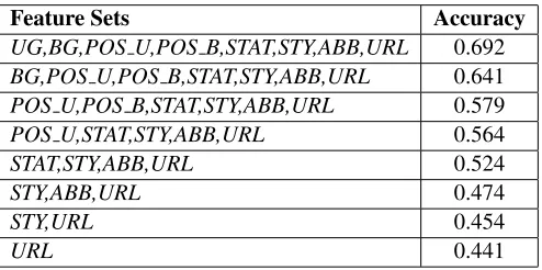
UG,BG,POS U,POS B,STAT,STY,ABB,URL 0.692
BG,POS U,POS B,STAT,STY,ABB,URL 0.641
POS U,POS B,STAT,STY,ABB,URL 0.579
POS U,STAT,STY,ABB,URL 0.564
STAT,STY,ABB,URL 0.524
STY,ABB,URL 0.474
STY,URL 0.454
[image:3.612.314.561.70.193.2]URL 0.441
Table 1: Cross validation average accuracy with differ-ent feature sets. we started with all 8 feature sets and removed feature sets one by one, where we always first removed the feature set that resulted in the biggest drop in accuracy.
4
Methods
In this section we describe the methods used by our system.
Firstly, we did feature selection on all the features described in Section 2. Using Mutual Information
(Shannon and Weaver, 1949) and 10-fold cross vali-dation we chose the top 13,500 features. Using these features we trained an SVM classifier with the train-ing data. As the implementation of the SVM classi-fier we usedliblinear(Fan et al., 2008). The SVM classifier was then used to produce initial predictions for messages in the development set, the Twitter test set and the SMS test set.
Then, we represented every message in the devel-opment set, the Twitter test set and the SMS test set using the 42 votes we described in Section 3 together with the predictions of the SVM classifier we described above. Using the Bagging algorithm from the WEKA machine learning toolkit (Hall et al., 2009) and the development set data, we trained a new classifier and used this classifier for the final prediction on Twitter test data and SMS test data.
5
Results
5.1 Feature analysis
Feature Sets Accuracy
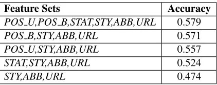
POS U,POS B,STAT,STY,ABB,URL 0.579
POS B,STY,ABB,URL 0.571
POS U,STY,ABB,URL 0.557
STAT,STY,ABB,URL 0.524
[image:4.612.87.298.69.152.2]STY,ABB,URL 0.474
Table 2: Cross validation average accuracy with further combination of feature sets.
Accuracy F1 (pos, neg)
Majority Baseline 0.4123 0.2919 SVM Classifier 0.6612 0.5414 SVM + LM Votes 0.6457 0.5384
Table 3: Overall accuracy and average F1 score for posi-tive and negaposi-tive classes on Twitter test data.
and used average accuracy as a metric.
As we can see from Table 1, lexical features were the most important features – they counted for more than 0.11 loss of accuracy when removed from the features. POS features and statistical features were also important, POS bigrams more so than POS uni-grams. Stylistic, abbreviation and URL features, on the contrary, seem to be only of moderate useful-ness.
To further investigate the relationship between the feature sets POS U, POS B and STAT, we did addi-tional experiments. From Table 2, we can see that removing all three feature sets caused a decrease in accuracy to 0.47, including just one feature set POS B, POS U or STAT resulted in accuracy above 0.57, 0.55 and 0.52 respectively. This shows that all three feature sets were quite effective and POS B was most useful. However, adding all of the three feature sets only caused an increase in accuracy to 0.579, which suggests that they were highly corre-lated.
Accuracy F1 (pos, neg)
Majority Baseline 0.2350 0.1902 SVM Classifier 0.6504 0.5811 SVM + LM Votes 0.6418 0.5670
Table 4: Overall accuracy and average F1 score for posi-tive and negaposi-tive classes on SMS test data.
5.2 Effectiveness of language model features
To evaluate the effectiveness of features derived from language models of character n-grams, we compared the performance of our SVM classifier and that of the classifier combining the SVM clas-sifier results and language model features.3We per-formed our experiments on both of the Twitter test data and the SMS test data. The results in Table 3 and Table 4 suggested that in our current setup, lan-guage model features were not very helpful.
Table 3 and Table 4 also show that our system improved the performance greatly compared to Ma-jority baseline system,4. Compared with other par-ticipants in the SemEval-2013 Task 2, our system achieved average performance on Twitter test data. However, it has been the ninth best out of all 48 sys-tems for the performance on SMS test data. This shows that our system can be easily adapted to dif-ferent contexts without a big drop in performance. One reason for that might be that we did not use any sentiment lexicon developed specifically for Twitter data and we used high level features like the statisti-cal features and POS features for our classification.
6
Conclusion
This paper briefly reports our system designed for the SemEval-2013 Task 2: sentiment analysis in Twitter. We first used an SVM classifier with a wide range of features. We found that simple statistics of the tweets, for example word count or readabil-ity scores, can help in sentiment analysis on Twitter text.
We then used character n-gram language mod-els to address the problem of high lexical variation in Twitter text and combined the two approaches to obtain the final results. Although in our current setup, features derived from character n-gram lan-guage models do not perform very well, they may benefit from a larger training data set.
Acknowledgments
This work was funded by DFG projects SFB 732. We would like to thank our colleagues at IMS.
3We accidentally used feature set POS B two times in our
representation, but it didn’t change the results significantly.
4To be consistent with the evaluation metric, we chose the
References
Fotis Aisopos, George Papadakis, Konstantinos Tserpes, and Theodora Varvarigou. 2012. Content vs. context for sentiment analysis: a comparative analysis over microblogs. InProceedings of the 23rd ACM confer-ence on Hypertext and social media, HT ’12, pages 187–96, New York, NY, USA. ACM.
Luciano Barbosa and Junlan Feng. 2010. Robust senti-ment detection on twitter from biased and noisy data. InProceedings of the 23rd International Conference on Computational Linguistics: Posters, COLING ’10, pages 36–44, Stroudsburg, PA, USA. Association for Computational Linguistics.
Albert Bifet and Eibe Frank. 2010. Sentiment knowl-edge discovery in twitter streaming data. In Proceed-ings of the 13th international conference on Discov-ery science, DS’10, pages 1–15, Berlin, Heidelberg. Springer-Verlag.
Dmitry Davidov, Oren Tsur, and Ari Rappoport. 2010. Enhanced sentiment learning using twitter hashtags and smileys. InProceedings of the 23rd International Conference on Computational Linguistics: Posters, COLING ’10, pages 241–249, Stroudsburg, PA, USA. Association for Computational Linguistics.
Rong-En Fan, Kai-Wei Chang, Cho-Jui Hsieh, Xiang-Rui Wang, and Chih-Jen Lin. 2008. LIBLINEAR: a li-brary for large linear classification. J. Mach. Learn. Res., 9:1871–1874, June.
Alec Go, Richa Bhayani, and L. Huang. 2010. Exploit-ing the unique characteristics of tweets for sentiment analysis. Technical report, Technical Report, Stanford University.
Mark Hall, Eibe Frank, Geoffrey Holmes, Bernhard Pfahringer, Peter Reutemann, and Ian H. Witten. 2009. The WEKA data mining software: an update. SIGKDD Explor. Newsl., 11(1):10–18, November. Bernard J. Jansen, Mimi Zhang, Kate Sobel, and Abdur
Chowdury. 2009. Twitter power: Tweets as elec-tronic word of mouth. J. Am. Soc. Inf. Sci. Technol., 60(11):2169–2188, November.
Long Jiang, Mo Yu, Ming Zhou, Xiaohua Liu, and Tiejun Zhao. 2011. Target-dependent twitter sentiment clas-sification. InProceedings of the 49th Annual Meet-ing of the Association for Computational LMeet-inguistics: Human Language Technologies - Volume 1, HLT ’11, pages 151–160, Stroudsburg, PA, USA. Association for Computational Linguistics.
Kun-Lin Liu, Wu-Jun Li, and Minyi Guo. 2012. Emoti-con smoothed language models for twitter sentiment analysis. InTwenty-Sixth AAAI Conference on Artifi-cial Intelligence.
A. Pak and P. Paroubek. 2010. Twitter as a corpus for sentiment analysis and opinion mining.LREC.
Bo Pang, Lillian Lee, and Shivakumar Vaithyanathan. 2002. Thumbs up? sentiment classification using ma-chine learning techniques. InProceedings of EMNLP, pages 79–86.
Stephan Raaijmakers and Wessel Kraaij. 2008. A shal-low approach to subjectivity classification. Proceed-ings of ICWSM, pages 216–217.
Robert Remus. 2011. Improving sentence-level subjec-tivity classification through readability measurement. May. Proceedings of the 18th Nordic Conference of Computational Linguistics NODALIDA 2011. Hassan Saif, Yulan He, and Harith Alani. 2012.
Seman-tic sentiment analysis of twitter. In Philippe Cudr-Mauroux, Jeff Heflin, Evren Sirin, Tania Tudorache, Jrme Euzenat, Manfred Hauswirth, Josiane Xavier Parreira, Jim Hendler, Guus Schreiber, Abraham Bern-stein, and Eva Blomqvist, editors,The Semantic Web ISWC 2012, number 7649 in Lecture Notes in Com-puter Science, pages 508–524. Springer Berlin Heidel-berg, January.
Claude E. Shannon and Warren Weaver. 1949. Mathe-matical Theory of Communication. University of Illi-nois Press.
Andreas Stolcke. 2002. SRILMAn extensible language modeling toolkit. InIn Proceedings of the 7th Inter-national Conference on Spoken Language Processing (ICSLP 2002, page 901904.
Andranik Tumasjan, Timm O. Sprenger, Philipp G. Sand-ner, and Isabell M. Welpe. 2010. Predicting elections with twitter: What 140 characters reveal about politi-cal sentiment.Proceedings of the Fourth International AAAI Conference on Weblogs and Social Media. Theresa Wilson, Zornitsa Kozareva, Preslav Nakov, Sara