Persistent current and Drude weight for the one-dimensional Hubbard model from current
lattice density functional theory
This article has been downloaded from IOPscience. Please scroll down to see the full text article. 2012 J. Phys.: Condens. Matter 24 055602
(http://iopscience.iop.org/0953-8984/24/5/055602)
Download details:
IP Address: 134.226.252.155
The article was downloaded on 07/03/2012 at 16:32
Please note that terms and conditions apply.
J. Phys.: Condens. Matter24(2012) 099601 (1pp) doi:10.1088/0953-8984/24/9/099601
Erratum: Persistent current and Drude
weight for the one-dimensional Hubbard
model from current lattice density
functional theory
2012
J. Phys.: Condens. Matter
24
055602
A Akande and S Sanvito
School of Physics and CRANN, Trinity College, Dublin 2, Ireland
E-mail:[email protected]
Received 31 January 2012 Published 13 February 2012
[image:2.595.83.257.415.644.2]Online atstacks.iop.org/JPhysCM/24/099601
Figure 5 of the original article should have been replaced with figure 5 below.
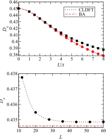
Figure 5. Drude coefficientDcas a function of the interaction strengthU/t(top panel) and of the number of sites in the ring,L (bottom panel). All the calculations are for quarter filling and the results in the top panel are for a 60-site ring. In the figure we compare CLDFT results (dotted black lines) with those obtained by the BA technique in the thermodynamic limit (dashed red lines). Calculations in the lower panel are forU/t=2.
IOP PUBLISHING JOURNAL OFPHYSICS:CONDENSEDMATTER
J. Phys.: Condens. Matter24(2012) 055602 (12pp) doi:10.1088/0953-8984/24/5/055602
Persistent current and Drude weight for
the one-dimensional Hubbard model from
current lattice density functional theory
A Akande and S Sanvito
School of Physics and CRANN, Trinity College, Dublin 2, Ireland
E-mail:[email protected]
Received 18 August 2011, in final form 1 December 2011 Published 17 January 2012
Online atstacks.iop.org/JPhysCM/24/055602
Abstract
The Bethe ansatz local density approximation (LDA) to lattice density functional theory (LDFT) for the one-dimensional repulsive Hubbard model is extended to current-LDFT (CLDFT). The transport properties of mesoscopic Hubbard rings threaded by a magnetic flux are then systematically investigated by this scheme. In particular we present calculations of ground state energies, persistent currents and Drude weights for both a repulsive homogeneous and a single impurity Hubbard model. Our results for the ground state energies in the metallic phase compare favorably well with those obtained with numerically accurate many-body techniques. Also the dependence of the persistent currents on the Coulomb and the impurity interaction strength, and on the ring size are all well captured by LDA-CLDFT. Our study demonstrates the value of CLDFT in describing the transport properties of one-dimensional correlated electron systems. As its computational overheads are rather modest, we propose this method as a tool for studying problems where both disorder and interaction are present.
(Some figures may appear in colour only in the online journal)
1. Introduction
Quantum dots, routinely made by electrostatically confining a two-dimensional electron gas [1], have been extensively studied in recent years [2]. The interest in these low-dimensional structures stems from the fact that their physics is controlled by quantum effects. Furthermore, while sharing many similarities with real atoms, quantum dots manifest intriguing low-energy quantum phenomena, which are specific to them. This is because their properties can be influenced by external factors such as the geometry or the shape of the confining potential and the application of external fields. Clearly some of these features are not accessible in real atoms. Research in the past has been motivated by the possibility of developing novel quantum dot based devices in both the fields of quantum cryptography/computing [3] and spintronics [4], as well as by the simple curiosity of exploring the properties of many-electron systems in reduced dimensions.
Quantum rings represent a particular class of quantum dots [5,6], where electrons are confined in circular regions [7,8]. The circular geometry can sustain an electrical current, which in turn can be induced by threading a magnetic flux across the ring itself. Such a magnetic flux produces exciting effects such as Aharonov–Bohm (AB) oscillations [9, 10] and persistent currents [11], effects that have been earlier anticipated [12–14]. In one dimension (1D) the persistent currents have been thoroughly studied [11, 15–20]. These, as well as many other physical properties of the ring, are a periodic function of the magnetic flux quantum,80=hc/e(h
is Planck’s constant,cthe speed of light andethe electron’s charge).
A number of earlier theoretical studies [16–20] on persistent currents focused on unveiling the role of electron correlations and disorder over the electron transport. This line of research is inspired by the fact that electronic correlation in 1D always leads to non-fermionic low-energy quasi-particle excitations. In fact, even in the presence of weak interaction, 1D fermions behave differently from a Fermi liquid and their
1
ground state is generally referred to as a Luttinger liquid. This possesses specific collective excitations [21].
There are two theoretical frameworks commonly used to study finite 1D rings [22]. The first is based on the continuum model, where electrons move in a uniform neutralizing positive background and interact via Coulomb repulsion, e2/4πε0r (ε0 is the vacuum permittivity, e the
electron charge, rthe distance between two electrons). The second framework is populated by lattice models, where the electronic structure is written in a tight-binding form and the electron–electron interaction is commonly described at the level of the Hubbard Hamiltonian [23, 24]. In both frameworks exact diagonalization (ED) has been the preferential solving strategy for small systems (small number of sites and electrons) [19, 25]. Additional methods used to study quantum rings over lattice models include the Bethe ansatz (BA) [26,27], renormalization group [28] and density matrix renormalization group [29, 30]. In contrast, the continuum model has been tackled with self-consistent Hartree–Fock techniques [31], bosonization schemes [32], conformal field theory [33], current-spin density functional theory [34] and quantum Monte Carlo methods [35].
Many of the methods developed for solving lattice models for interacting electrons suffer from a number of intrinsic limitations connected either to their large computational overheads or to the need of using a drastically contracted Hilbert space. Density functional theory (DFT) can be a natural solution to these limitations. DFT is a highly efficient and precisely formulated method [36,37], originally developed for the Coulomb interaction (this is commonly known as ab initio DFT) and then extended to lattice models [38–40]. Lattice DFT (LDFT) is based on the rigorously proved statement that the ground state of an interacting electron system is a universal functional of the local site occupation. The functional, as in ab initio
DFT, is unknown explicitly. However, all the many-body contributions to the total energy can be incorporated in a single term, the exchange and correlation (XC) energy, for which a hierarchy of approximations can be constructed.
The most commonly used approximation for the XC energy in ab initio DFT is probably the local density approximation (LDA) [37, 41], where the exact (unknown) XC energy is replaced by that of the homogeneous electron gas. The theory is then expected to work best in situations close to those described by the reference system, i.e. close to the homogeneous electron gas. Since in a 1D Fermi liquid theory breaks down, the homogeneous electron gas is no longer a good reference. For the homogeneous Hubbard model it was then proposed [40, 42] to use instead the BA construction of Lieb and Wu [27]. Such a scheme was then applied successfully to a wide range of situations [43–49] and more recently it has been extended to time-dependent problems [48,50–52] and to the 3D Hubbard model [53].
LDFT can be further extended to include the action of a vector potential, i.e. it can be used to tackle problems where a magnetic flux is relevant. This effectively corresponds to the construction of current-LDFT (CLDFT). Such an extension of LDFT was proposed recently for
one-dimensional spinless fermions with nearest-neighbor interaction [54]. Furthermore, very recently Tokatly has presented a rigorous formulation of time-dependent current DFT (TDCDFT) on a lattice [55] similar to an earlier work based on power series construction [56].
In the present work, we extend the CLDFT construction of [54] to the repulsive Hubbard model. The newly proposed functional is then used to investigate total energies, persistent currents and Drude weights of a mesoscopic ring threaded by a magnetic flux. These quantities are compared with the same calculated by exact methods, namely by exact diagonalization for small systems and by asymptotically exact expressions for large ones. Such a benchmark exercise is one of the main contributions of this work, which determines the level of accuracy of CLDFT in describing electron transport problems. In addition we investigate the scaling properties of both the persistent currents and the Drude weights with the ring length and the interaction strength. In particular we are able to propose a complete scaling law for both the persistent current and the Drude weight as a function of ring size and interaction strength in the metallic limit of the Hubbard model.
Notably these tests return us a functional capable of describing at the quantitative level the Hubbard model in a magnetic field in the metallic limit. Considering the fact that our CLDFT scales cubically with the number of atomic sites (the scaling can be made linear by using more sophisticated matrix diagonalization techniques), in contrast with the exponential scaling of many-body numerical schemes, CLDFT appears to be an intriguing option for investigating problems involving large ensemble averages. Electron conduction in disorder systems or in the presence of electron–phonon coupling appears as two natural choices and they will be explored in the future.
The paper is organized as follows. Section 2 reviews the theoretical foundations leading to the construction of CLDFT and to its LDA. Then we present our results for both homogeneous and defective rings, highlighting the main capabilities and limitations of our scheme, and finally we conclude.
2. Theoretical formulation of current lattice DFT
Current DFT (CDFT) is a generalization of the DFT formalism to Hamiltonians that include an external vector potential, i.e. it is a generalization of the theory to external magnetic fields [57]. In this case the theory is constructed over two fundamental quantities, namely the electron density,n, and the paramagnetic current density,Ejp. The Hohenberg–Kohn theorem [36] is thus expanded to the statement that the ground statenandEjpuniquely determine the
ground state wavefunction and consequently the expectation values of all the operators [58, 59]. Equally important is the fact that the standard Kohn–Sham construction can also be employed for CDFT, so that the many-body problem can be mapped onto a fictitious single-particle one, with the two sharing the same ground state n and Ejp [58, 59].
J. Phys.: Condens. Matter24(2012) 055602 A Akande and S Sanvito
of the theory are incorporated in the XC energy, which then needs to be approximated.
The scope of this section is to describe how ab initio
CDFT has been translated to lattice models and how a suitable approximation for the Hubbard Hamiltonian in 1D can be constructed. Note that a similar formulation can be elaborated also in higher dimensions, although the lack of exact results makes the construction of suitable approximations much more problematic as one depends only on numerical analysis for small systems. Our description follows closely the one previously given by Dzierzawa et al [54]. In general a vector potential, AE, enters into a lattice model via Peierls substitution [60, 61], where the matrix elements of the
E
A-dependent Hamiltonian, H(Er,Ep + e
cAE), can be written in
terms of those forAE=0 as
h ER0|HEr,Ep+e
c
E
A| ERi = h ER0|H(Er,Ep)| ERie−hci¯e RRE0
E
R A·EdEs, (1)
wherec is the speed of light and | ERi is the generic orbital located at the position RE and belonging to the basis set
(here assumed orthogonal) used to construct the tight-binding Hamiltonian.
When the Peierls substitution is applied to the construction leading to the 1D Hubbard model the only term in the Hamiltonian that gets modified is the kinetic energyTˆ. This takes the form
ˆ
T = −t L
X
σ,l=1
(e−i8σl/Lcˆσ†l+1cˆσl+hc), (2)
where we have considered a system comprised ofL atomic sites (note that the ring boundary conditions implyL+1=1). In equation (2),ˆc†σl(cˆσl) is the creation (annihilation) operator
for an electron of spin σ (σ =↑,↓) at the l-site, t is the hopping integral and8σl is the phase associated with thelth
bond, which effectively describes the action of AE. Here hc
denotes the hermitian conjugate. The remaining terms in the Hamiltonian are unchanged so that the 1D Hubbard model in the presence of a vector potential is defined by
ˆ
HHubbard8 = ˆT+ ˆU+
L
X
l
vextl nˆl, (3)
where {vextl } is the external potential (vextl is the on-site energy of the l-site), while the Coulomb repulsion term is
ˆ
U =UPL
l=1n↑lˆ n↓lˆ , with U being the Coulomb repulsion
energy and nˆσl = ˆc†σlcˆσl. Throughout this work we always
consider the diamagnetic (non-spin-polarized) case so that
8↑l=8↓l =8landn↑l=n↓l=nl.
The first step in the construction of a CLDFT is the formulation of the problem in a functional form. The basic variables of the theory are the site occupationnl = h9| ˆnl|9i
and bond paramagnetic current, jl = h9|ˆjl|9i, where |9i
is the many-body wavefunction and the bond paramagnetic current operator is defined as
ˆ
jl= −it(e−i8l/Lcˆ†σl+1cˆσl−hc). (4)
In complete analogy toab initioCDFT we can write the total energy,E, of the Hamiltonian (3) as a functional of the local external potentials and phases
E=F[nl,jl] +X
l
vextl nl+X
l
8ljl, (5)
so that
nl= h ˆnli = ∂E
∂vextl , jl= hˆjli = ∂E
∂8l. (6)
F[nl,jl] is a universal functional, in the sense that it does not depend on the external potentialvext, although note that one has a different F[nl,jl] for every U/t. The functional
derivatives ofF[nl,jl]with respect to{nl}and{jl}satisfy the
following two equations
vextl = −∂F
∂nl
8l= −∂F
∂jl
. (7)
Note that equations (5) through (7) follow directly from the properties of the Legendre transformation.
In order to make the theory practical one has now to introduce the auxiliary single-particle Kohn–Sham system. This is described by a single-particle Hamiltonian,Hˆs, whose ground state site occupations and bond paramagnetic currents are identical to those of the interacting system (described by equation (3)).Hˆsreads
ˆ
Hs= ˆTs+
L
X
l
vslnˆl, (8)
where Tˆs = −tPL−1
σ,l=1(e
−i8sl/Lcˆ†
σl+1ˆcσl + hc) and the
associated local effective potentials and phases arevsl and8sl respectively. The single-particle Schr¨odinger equation is then
ˆ
Hs|9αsi =α|9αsi, (9)
and the site occupation is defined as
nsl =X
α
fαh9αs| ˆnl|9αsi, (10)
wherefα is the occupation number. An analogous expression can be written forjsl.
The energy functional associated with the Kohn–Sham system, Fs, can be constructed by performing again a
Legendre transformation
Fs =Es−X
l
vslnsl −X
l 8s
ljsl, (11)
whereEs is the total energy of the single-particle system and
the following two equations are valid
vsl = −∂F s
∂nsl , 8
s
l = − ∂Fs
∂jsl . (12)
The crucial point is that in the ground state the real and the Kohn–Sham systems share the same site occupation and paramagnetic current, i.e.nl=nsl andjl=jsl.
Thus one is now in the position of defining the XC energy, Exc, as usual, i.e. as the difference between F for
the interacting and the Kohn–Sham systems after the classical Hartree energyEHhas also been subtracted,
Exc[nl,j
l] =F[nl,jl] −Fs[nl,jl] −EH[nl]. (13)
Note that for all the functionals in equation (13) we took the short notation {nl} →nl and {jl} →jl, i.e. the functionals
depend on all the on-site occupations and bond paramagnetic currents. The single-particle effective potentials and phases can now be defined. In fact by taking the functional derivative of equation (13) with respect to nl and jl and by using the
equations (7) and (12) one obtains
vsl =vextl +vHl +vxcl , 8sl =8l+8xc
l , (14)
where
vxcl =∂E xc
l ∂nl
, 8xc
l = ∂Exc
l ∂jl
, (15)
andvHl =∂EH
l /∂nl(=Unl/2) is the Hartree potential.
FinallyExccan be re-written in terms of the expectation
values of the original Hamiltonian. In fact by substituting the functional forms ofFandFsinto the equation (13),
Exc=E−Es+X
l
(vsl −vextl )nl
+ X
l (8s
l −8l)jl−EH[nl], (16)
by using the equations (3) and (8),
X
l
(vsl−vextl )nl=Es−E− h9s| ˆTs|9si + h9| ˆT+ ˆU|9i,
(17)
and again by substituting equation (17) into (16), one obtains a close expression for the XC energy
Exc= h9| ˆT+ ˆU|9i − h9s| ˆTs|9si
+ X
l (8s
l −8l)jl−EH[nl]. (18)
Once the theory is formally established the remaining task is that of finding an appropriate approximation forExc. As
for the case of standard LDFT [42,43], the strategy here is that of considering the BA solution for the homogeneous limit of
ˆ
H8Hubbard(this is defined in equation (3) by settingvl=vand
8l=8) and then of taking its local density approximation
n→nl,8→8l[54], i.e.
ELDAxc [nl,jl] =
X
l
exc[nl,jl], (19)
where exc[n,j] = Exc[n,j]/L is the XC energy density
(per site) of the homogeneous system. The first term of the equation (18) can be calculated exactly using the BA procedure [62]. This provides the ground state energy as a function ofn and8, so that one still needs to re-express it in terms of n andj. However, the phase variable 8 can be eliminated from the ground state energy by using
j= ∂E(n, 8)
∂8 . (20)
Thus, finally one can explicitly write exc(n,j)(the full derivation for the 1D Hubbard Hamiltonian is presented in the appendix)
exc(n,j)=exc(n,0)+1 23
xc(n)j2, (21)
where
exc(n,0)= E
BA(n,0)−E0(n,0)−EH(n)
L ,
3xc(n)= 1
2 1
D0 c(n)
− 1
DBA c (n)
.
(22)
In the equations above E0(n,0) andD0
c(n)are respectively
the non-interacting ground state energy and charge stiffness, while EBA(n,0)andDBA
c (n)are the same quantities for the
interacting case as calculated from the BA. Finally, the XC contributions to the Kohn–Sham potential can be obtained by a simple functional derivative (in this case by a simple derivative) of the exchange and correlation energy density with respect to the fundamental variablesnandj, i.e. they are
vxc(n,j)= ∂e xc(n,j)
∂n =v
xc 1(n,0)+
1
2v
xc 2(n)j
2,
8xc(n,j)=∂exc(n,j)
∂j =3xc(n)j,
(23)
where
vxc1(n,0)=∂e xc(n,0)
∂n , v
xc 2(n)=
∂3xc(n)
∂n . (24)
Then, by taking the LDA one obtains
vxcBALDA(nl,jl)=vxc(n,j)|n→nl,j→jl
8xc
BALDA(nl,jl)=3xc(n)j|n→nl,j→jl,
(25)
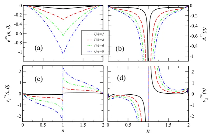
where BALDA, as usual, stands for Bethe ansatz LDA. In the panels of figure 1 we present exc(n,0), 3xc(n),
vxc1 (n,0)andvxc2(n)as a function of the electron density,n, for different interaction strengthsU/t. As in the case of standard LDFT also for CLDFT there is a divergence in then-derivative of both exc(n,0) and 3xc(n) at half-filling (n =1), which results in a discontinuity of bothvxc1 (n,0)andvxc2 (n). Such a discontinuity arises in correspondence of the metal–insulator transition present in the 1D Hubbard model for finite U/t. Importantly in the case of 3xc(n)the divergence is also in
3xc(n)itself.
The solution of the Kohn–Sham problem proceeds as follows. First an initial guess for the site occupations is used to construct the initial local paramagnetic current density. Then, the functional derivatives of equations (25) are evaluated at these given n and j so that the Kohn–Sham potential is constructed. The Kohn–Sham equations are then solved to obtain the new set of Kohn–Sham orbitals from which the new orbital occupations and bond paramagnetic currents are calculated (by using equation (10)). The procedure is then repeated until self-consistency is reached, i.e. until the potentials (or the densities) at two consecutive iterations vary below a certain threshold. After convergence is achieved the total energy for the interacting system is calculated from
E =X
α
fαα +Exc[nl,j
l] −EH[nl] −
X
l
J. Phys.: Condens. Matter24(2012) 055602 A Akande and S Sanvito
Figure 1. The XC energy density (per site) and potential for a homogeneous 1D Hubbard ring threaded by a magnetic flux as a function of the electron density and for different values of interaction strengthU/t: (a) exc(n,0), (b)3xc(n), (c)vxc1(n,0)and (d)vxc2(n).
where the first term is the sum of single-particle energies and the other terms are the so-called double counting corrections.
3. Results and discussion
We now discuss how CLDFT performs in describing both the energetics and the transport properties of 1D Hubbard rings in the presence of a magnetic flux. For small rings our results will be compared with those obtained by diagonalizing exactly the Hamiltonian of equation (3), while CLDFT for large rings will be compared with the BA solution. First we will consider homogeneous rings and then we will explore the single impurity problem. Note that this analysis, exploring both small sizes and the approach to the thermodynamic limit, is crucial for establishing the universality of our constructed functional. It is very much in the spirit of testing the LDA in standardab initioDFT, where the theory is exact for the homogeneous gas, but extrapolated for situations where the density is not homogeneous, e.g. molecules, atoms, surfaces etc.
3.1. Homogeneous rings: general properties
In this section we focus our attention on discussing the general features of CLDFT applied to homogeneous Hubbard rings threatened by a magnetic flux, i.e. on the performance of CLDFT in describing the Aharonov–Bohm effect. We start our analysis by comparing the CLDFT results with those obtained by ED. Since ED is numerically intensive such a comparison is limited to small systems.
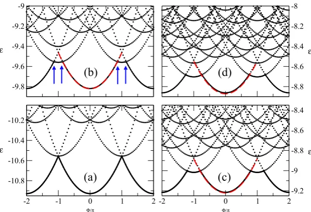
In figure2we present the first low-lying energy levels,E, calculated by ED as a function of the magnetic flux,8, for a small 12-site ring at quarter filling (n=1/2). In particular we present results for the non-interacting case (panel (a)) and for the interacting one at three different interaction strengths:
(b)U/t=2, (c)U/t=4 and (d)U/t=6. Exact results (ED) are in black, while those obtained with CLDFT in red. In general the ground state energy is minimized at8=0 when the number of electrons is N=4m+2 and at 8=π for
N =4m, withmbeing an integer [63]. Here we consider the caseN=4m+2 where the ground state is a singlet [64].
For non-interacting electrons,U/t=0, the total energy of the singlet ground state is a parabolic function of8. Also the various excited states have a parabolic dependence on8 and simply correspond to single-particle levels with different wavevectors. As the electron–electron interaction is turned on the non-interacting spectrum gets modified in two ways. Firstly there is a second branch in the ground state energy as a function of 8 appearing at around 8= ±π (see the blue arrows in panel (b) of figure2). This originates from the degeneracy lifting between the single and the triplet solution at8= ±π, with the triplet being pushed down in energy and becoming the ground state. The8region where the ground state is a triplet widens as the interaction strengths increases. The second effect is the expected increase of the absolute value of the ground state total energy asU/tincreases.
Since CLDFT is a ground state theory, it provides access only to the ground state energy,E. This is calculated next and plotted in figure2in the interval−π ≤8≤π for different
U/t. As one can clearly see from the figure, the performance of CLDFT is rather remarkable, to a point that the CLDFT energy is practically identical to that calculated with ED. However, CLDFT completely misses the cusps in the E(8)
profile arising from the crossover between the singlet and the triplet state. Level crossing invalidates the BA approximation, leading to the interacting XC energy (see equations (37) in the appendix) and so failures are expected [65]. This observation is in agreement with earlier studies [22] in which the inability of CDFT to reproduce level crossing was already noted. Also note that our formulation is non-spin polarized, so that triplet states cannot be described. This unfortunately is a present
Figure 2. The low-lying energy spectrum,E, of a 12-site ring at quarter filling (n=1/2) as a function of the magnetic flux,8, and calculated for different interaction strengthsU/t. The black dotted lines represent ED results while the dashed red ones are for CLDFT. Note that for the non-interacting case,U/t=0, in panel (a) there is no difference between CLDFT and ED. Panels (b)–(d) are for the interacting case at different interaction strengths: (b)U/t=2, (c)U/t=4 and (d)U/t=6. In panel (b) the blue arrows indicate the region where the triplet state becomes the ground state.
limitation of the method. Here we just wish to point out that the formulation of a spin-polarized LDFT is in its infancy even for the case where no vector potential is included [66]. With all this in mind, as long as the singlet remains the ground state, the agreement between CLDFT and ED results is remarkable, even if this small ring is rather far from being a good approximation of the thermodynamic limit (the BA solution) upon which the functional has been constructed.
Having calculated the total energies with both ED and CLDFT, the corresponding persistent currents, j, can be obtained by taking the numerical derivative of E(8) with respect to8. In figure3we show results for the 12-site ring at quarter filling (n =1/2), whose total energy was presented in figure 2. In particular we plot j only over the period
−π < 8 < π, since all the quantities are 2π periodic. The figure confirms the linearity of the persistent currents with the magnetic flux for all the interaction strengths considered. The same is also true for other fillings for the 12-site ring (not presented here) away from half-filling. We also observe that the magnitude of persistent currents reduces with increasing
U/tfor both ED and CLDFT and that the precise dependence of j on U/t is different for different fillings. This is in good agreement with previous calculations based on the BA technique [67].
ED is computationally demanding and cannot be performed beyond a certain system size. For this reason, in order to benchmark CLDFT for larger rings, we have calculated the ground state energy with the BA method. An example of these calculations is presented in figure 4, where once again we show E(8)for L=20, U/t=4 and different numbers of electrons. Also in this case the agreement between the BA results and those obtained with CLDFT is remarkably good as long as the ground state is a singlet. Interestingly we note that the agreement is better for low
Figure 3. Persistent current profile,j, for a 12-site ring at quarter filling (n=1/2) obtained with both ED and CLDFT for different
U/t. The full lines are thejcalculated with ED while the dashed ones are for CLDFT.
filling but it deteriorates as one approaches the half-filling case (N=20 in this case). This is somehow expected given the discontinuity of3xcand of the derivative of excatn=1 (see figure 1), leading to the Mott transition. The presence of these discontinuities, although qualitatively correct, poses numerical problems and losses in accuracy.
The final quantity we wish to consider is the charge stiffness or Drude weight,Dc, defined as
Dc=
L
2
∂2E(n, 8)
∂82
8=0.
(27)
[image:8.595.311.543.358.525.2]J. Phys.: Condens. Matter24(2012) 055602 A Akande and S Sanvito
Figure 4. Ground state energy,E(8), as a function of the magnetic flux,8, calculated with both the BA technique (dotted black line) and CLDFT (dashed red line). Calculations are carried out forL=20,U/t=4 and different numbers of electrons: (a)N=2 (n=1/10), (b)N=6 (n=0.3), (c)N=10 (n=1/2) and (d)N=14 (n=0.7).
long-wavelength limit (see appendix for more details). Dc
determines both qualitatively and quantitatively the transport properties of the ring. Importantly in the limit of large rings it exponentially vanishes for insulators, while it saturates to a finite value for metals. Many studies have been devolved to calculatingDcfor interacting systems. R¨omer and Punnoose
have studiedDcfor finite Hubbard rings using an iterative BA
technique [65]. Eckernet alexplored the relation betweenDc
and the so-called phase sensitivity,1E, for spinless fermions.
1E is the difference in the total energy calculated at8=0 (periodic ground state) and that at8=π(antiperiodic ground state) [68, 69]. A similar approach has been earlier used to study the effect of disorder on persistent current for the Hubbard model at half-filling [70]. Recently a density matrix renormalization group algorithm has been developed to deal with complex Hamiltonian matrices and used to calculateDc
for spinless fermions [30].
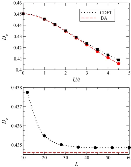
Since the agreement between CLDFT and ED is proved for small rings (the slopes of the persistent currents as a function of8calculated with CLDFT and ED are essentially identical in figure3) we concentrate here on a larger system, namely a homogeneous 60-site ring at quarter filling. Our results for the Drude weight as a function ofU/tare presented in figure5. Again the CLDFT data are compared with those calculated with the BA in the thermodynamic limit (L → ∞) and the agreement is rather satisfactory. We note that, as for the ground state energy, also for the Drude weight the CLDFT seems to perform less well as U/t increases, i.e. as the interaction strength becomes large. Then in the lower panel of figure5we illustrate the scaling properties of
Dc as a function of the number of sites in the ring, L (we
consider quarter filling and U/t =2). Clearly Dc does not
vanish at any lengths demonstrating that the system remains metallic. Furthermore it approaches a constant value already forL>40. In the picture we also report the asymptotic value predicted by the BA in the thermodynamic limitL→ ∞for
Figure 5. Drude coefficientDcas a function of the interaction
strengthU/t(top panel) and of the number of sites in the ring,L
(bottom panel). All the calculations are for quarter filling and the results in the top panel are for a 60-site ring. In the figure we compare CLDFT results (dotted black lines) with those obtained by the BA technique in the thermodynamic limit (dashed red lines). Calculations in the lower panel are forU/t=2.
this set of parameters. We find that the calculated CLDFT value is only 0.06% larger than the BA one, i.e. it is in quite remarkable good agreement.
[image:9.595.312.536.336.622.2]Figure 6. Persistent current,j, as a function of the number of sites in the ring,L, and for different electron occupations,n: (a)U/t=2, (b)U/t=4. Results are obtained with both the exact BA technique and CLDFT. In the figure the persistent currents are calculated at
8=π/2, i.e.j=j(π/2).
3.2. Scaling properties
Next we take a more careful look at the scaling properties of the persistent currents and the Drude weights as a function of both the ring size and the interaction strength. It is well known that j is strongly size dependent, since it originates from electron coherence across the entire ring [30]. For a perfect metal one expect jto scale as 1/L [25]. In figure 6 the value of the persistent currents as a function of the ring size are presented for different electron fillings and for the two representative interaction strengths ofU/t=2 (a) and
U/t=4 (b). Calculations are performed with both the exact BA and CLDFT. As a matter of convention we calculate the persistent currents at8=π/2.
In general we find a monotonic reduction of the persistent current with L and an overall excellent agreement between the BA and the CLDFT results over the entire range of lengths, occupations and interaction strengths investigated. A non-linear fit of all the curves of figure6returns us an almost perfect 1/Ldependence ofjwith no appreciable deviations at any n or U/t. This indicates a full metallic response of the rings in the region of parameters investigated, thus confirming previous results obtained with the BA approach [67].
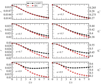
Then we look at the dependence of j and Dc on the
interaction strength. In this case we consider a 60-site ring and four different electron fillings. In general for small fluxes one expects j =2Dc8/L and our numerical results
of figure 7 demonstrate that this is approximately correct also for our definition of persistent currents (j =j(8 =
π/2)) over the entire U/t range investigated. We find that both j and Dc monotonically decrease as a function
of the interaction strength, essentially meaning that the predicted long-wavelength optical conductivity is reduced as the electron repulsion gets larger.
Also in this case the agreement between the BA and the CLDFT results is substantially good, although significant deviations appear in the limit of largeU/tand electron filling approaching half-filling. This again corresponds to a region of the parameter space where the XC potential approaches the derivative discontinuity.
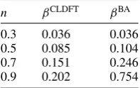
Table 1. Exponents for the empirical scaling laws of equation (28) as fitted from the data of figure7.
n βCLDFT βBA
0.3 0.036 0.036 0.5 0.085 0.104 0.7 0.151 0.246 0.9 0.202 0.754
It was numerically demonstrated in the past [67] that the persistent current (and so the Drude weight) at half-filling follows the scaling relationj∼e−U2/ξ, withξ ∼1. However, to the best of our knowledge, no scaling relation was ever provided in the metallic case. We have then carried out a fitting analysis (the fit is limited to values ofjandDcforU/t>2)
and found that our data can be well represented by the scaling laws
j=j0(U/t)−β, Dc=D0(U/t)−γ. (28)
In general and as expected we find β =γ and a quite significant dependence of the exponents on the filling. In particular table 1 summarizes our results and demonstrates that the decay rate of both the persistent currents and the Drude weights increases as the filling approaches half-filling. Note that β was extracted for rings containing 60 sites but the same fit repeated for L=40 gives almost identical results. Furthermore the table also quantifies the differences between the BA and the CLDFT solutions, whose exponents increasingly differ from each other as the electron filling gets closer to n =1 (for n =0.7 and n=0.9 we find βBA ∼
2βCLDFTandβBA∼4βCLDFTrespectively).
Finally, by combining all the results of this section we can propose a scaling law for both the persistent currents and the Drude weights, valid in the metallic limit of the Hubbard model, i.e. away from half-filling, and in the thermodynamic limit, i.e. forL1. This reads
j= j0(n)
L
U t
−β(n)
[image:10.595.377.476.300.362.2]J. Phys.: Condens. Matter24(2012) 055602 A Akande and S Sanvito
Figure 7. Persistent current,j, and Drude weight,Dcas a function of interaction strengthU/tfor a 60-site ring at different fillings. Results
are obtained with both the exact BA technique and CLDFT.
where both the constantj0 and the exponentβ are functions
of the electron fillingn. Note that an identical equation holds forDc.
3.3. Scattering to a single impurity
Having established the success of the BALDA to CLDFT for the homogeneous case we now move to a more stringent test of the theory, namely the case of a ring penetrated by a magnetic flux in the presence of a single impurity. Such a problem has already received considerable attention in the past [34, 71, 72]. Note that, as in ab initio DFT, this is a situation different from the reference system used to construct the BALDA (since it deals with a nonhomogeneous system) and therefore one might expect a more pronounced disagreement with the exact results. As the BA equations are integrable only for the homogeneous case we now benchmark our CLDFT results with those obtained by ED. This, however, limits our analysis to small rings.
The single impurity in the ring is described by simply adding to the Hamiltonian of equation (3) the term
ˆ
Himp=εimpnˆi, (30)
where εimp is the modification to the on-site energy at
the impurity site i. The inclusion of an impurity produces in general electron backscattering so that we expect the persistent currents to get reduced. In figure 8 we present the general transport features for this inhomogeneous system. Calculations have been carried out with CLDFT for a ring comprising 53 sites andN=26,U/t=4. Again the persistent currents are calculated at8=π/2.
Panel (a) shows j as a function of the impurity on-site energy. As expected from standard scattering theory the current is reduced asεimpincreases, thus creating a potential
barrier. The electron density profile for this situation is presented in panel (b), where one can clearly observe an electron depletion at the impurity site and Friedel’s oscillations around it.
A quantitative assessment of our CLDFT results is provided in figure 9 where they are compared with those obtained by exact diagonalization for a 13-site ring close to quarter filling (N =6). In particular we present j as a function of the impurity potential,εimp, for bothU/t=2 and
4. In general we find a rather satisfactory agreement between CLDFT and the exact results in particular for small εimp
andU/t. As the electron scattering becomes more significant deviations appear and the quantitative agreement is less good. Importantly we notice that the ED results systematically provide a persistent current lower than that calculated with CLDFT, at least for the values of electron filling investigated here. This seems to be a consistent trend also present for the homogeneous case (see figure7), although the deviations in that case are less pronounced (for the same electron filling and interaction strength).
We tentatively conclude that most of the errors in the impurity problem may be attributed to the errors already present in the homogeneous case. In addition we may speculate on the possible source of the additional errors specific to the scattering situation. Previous calculations for spinless fermions [54] point to the difficulties in applying the BALDA when backscattering is significant. Related to this issue is the fact that the exact XC functional, as in the case of standard LDFT [49], may be intrinsically nonlocal. This is
Figure 8. (a) Persistent current,j, as a function of single impurity strength,εimp, obtained from the CLDFT forL=53,N=26,U/t=4
and8= π
2. In (b) we show a typical site density profile for a positive single impurity site potential.
Figure 9. Comparison between the persistent currents calculated with CLDFT (black symbols and dotted line) and by ED (red symbols and dashed line) for a 13-site ring andN=6. Thejs are obtained at8=π/2 for two different values of the interaction strength, namely
U/t=2 (a) andU/t=4 (b).
an aspect that certainly deserves further investigation. In any case CLDFT already provides satisfactorily good results for the scattering problem and this is achieved only at a minor computational cost. As such CLDFT appears as the ideal tool for investigating the interplay between electron–electron interaction and disorder in low-dimensional structures.
4. Conclusion
In this work we have presented an extension of the BALDA for the one-dimensional Hubbard problem on a ring to CLDFT. We have then investigated the response of interacting rings to an external flux both in the homogeneous and inhomogeneous case, and we have compared our results with those obtained by numerically exact techniques. For the homogeneous case we have been able to extract a new scaling law as a function of chain length and interaction strength for both the persistent currents and the Drude weights at various electron fillings in the metallic limit.
In general we have found that CLDFT performs rather well in calculating both the persistent currents and the Drude weights in the homogeneous case. Furthermore a similar level of accuracy is transferred to the impurity problem. With these results in hand we propose to use CLDFT in the study of AB rings where the combined effect of electron–electron
interaction and disorder can be addressed for large rings, so that a numerical evaluation of the various scaling laws proposed in the past can be accurately carried out.
Acknowledgments
We thank N Baadji, I Rungger and V L Campo for useful discussions. This work is supported by the Science Foundation of Ireland under the grants SFI05/RFP/PHY0062 and 07/IN.1/I945. Computational resources have been provided by the HEA IITAC project managed by the Trinity Center for High Performance Computing and by ICHEC.
Appendix. Local density approximation for the
CLDFT
We use the BA solution for the homogeneous part of the
ˆ
HU8(equation (3)) to estimate the XC energy. Then the local approximation is taken,
Exc
LDA[nl,jl] =
X
l
exc[nl,jl]. (31)
Here exc(=Exc[n,j]
L ) is the XC energy per site for the
[image:12.595.144.453.273.412.2]J. Phys.: Condens. Matter24(2012) 055602 A Akande and S Sanvito
first term of the equation (18) can be calculated exactly using the BA procedures [62] to obtain the ground state energy as a function of n and 8. Then the phase variable 8 can be eliminated from the ground state energy to contain the current via
j= ∂E(n, 8)
∂8 . (32)
The complete flux dependence of the ground state energy for the Mott insulator phase (n=1) in the thermodynamic limit has been shown to be [64]
E(n, 8)−E(n,0)= 2Dc(n)
L (1−cos8), (33)
while away from half-filling andL→ ∞this is
E(n, 8)−E(n,0)=Dc(n)
L 8
2. (34)
HereDc(n)is the charge stiffness (Drude weight) defined as
Dc=
L
2
∂2E(n, 8)
∂82 8= 0 . (35)
In physical terms the Drude weightDcis the real part of the
optical conductivityσ1(w)in the long-wavelength limit [64],
σ1(w)=2πDcδ(w)+σ1reg(w), (36)
where we tookh¯ =e=c=1. If we denoteEBA(n
BA, 8BA)
and E0(n
0, 80)respectively as the ground state energy for
the interacting system (first term in equation (18)) and for the non-interacting one (second term in equation (18)), away from half-filling we will write
EBA(n
BA, 8BA)=EBA(nBA,0)+
DBAc (nBA)
L 8
2 BA,
E0(n0, 80)=E0(n0,0)+
D0c(n0)
L 8
2 0,
(37)
and
jBA(nBA, 8BA)=2
DBAc (nBA)
L 8BA,
j0(n0, 80)=2
D0c(n0)
L 80.
(38)
The fundamental requirement of the KS mapping is that
nBA =n0=nandjBA =j0=jwhile we note that8BA =8
and80=8sin equation (18). By substituting equations (37)
and the expressions for8sand8obtained from equation (38) into (18) one obtains
Exc(n,j)=EBA(n,0)−E0(n,0)−EH(n)
+L
23
xc(n)j2, (39)
where
3xc(n)=1
2 1
D0 c(n)
− 1
DBAc (n)
. (40)
HereD0c(n)is the non-interacting charge stiffness defined as
D0c(n)= 2t
π sin
nπ 2
(41)
for L → ∞. DBAc (n) can then be obtained in the thermodynamic limit by using [73]
DBAc (n)= 1
2π [ξc(Q)]
2v
c (42)
whereξc is an element of the dressed charge matrix, which
is used to describe the scattering between the quasi-particles andvcis the velocity of the charge excitation. Therefore one
finally obtains
exc(n,j)=exc(n,0)+1 23
xc(n)j2, (43)
so that
vxcBALDA(nl,jl)= ∂e xc(n,j)
∂n n→nl,j→jl (44) and 8xc
BALDA(nl,jl)=
∂exc(n,j)
∂j =3xc(n)j
n→nl,j→jl . (45)
References
[1] Davies J H 1998The Physics of Low-Dimensional
Semiconductor(Cambridge: Cambridge University Press) [2] See for example Andrey R (ed) 2008Semiconductor
Nanocrystal Quantum Dots, Synthesis, Assembly, Spectroscopy and Applications(Vienna: Springer)
Reimann S M and Manninen M 2002Rev. Mod. Phys.741283
Giamarchi T 2004Quantum Physics in One Dimension
1st edn (Oxford: Oxford University Press)
[3] Zipper E, Kurpas M, Szelkag M, Dajka J and Szopa M 2006
Phys. Rev.B74125426
[4] F¨oldi P, K´alm´an O, Benedict M G and Peeters F M 2006Phys. Rev.B73155325
[5] Lorke A, Luyken R J, Govorov A O, Kotthaus J P,
Garcia J M and Petroff P M 2000Phys. Rev. Lett.842223
[6] Fuhrer A, L¨usher S, Ihn T, Heinzel T, Ensslin K, Wegscheider W and Bichler M 2001Nature413822
[7] Garcia J M, Medeiros-Ribeiro G, Schmidt K, Ngo T, Feng J L, Lorke A, Kotthaus J and Petroff P M 1997Appl. Phys. Lett. 712014
[8] Lorke A and Luyken R J 1998PhysicaB256424
[9] Aharonov Y and Bohm D 1959Phys. Rev.115485
[10] Levy L P, Dolan G, Dunsmuir J and Bouchiat H 1990Phys. Rev. Lett.642074
[11] B¨uttiker M, Imry Y and Landauer R 1983Phys. Lett.A96365
[12] Hund F 1938Ann. Phys.32102
[13] Bloch F 1965Phys. Rev.137A787
[14] Bloch F 1968Phys. Rev.166415
[15] B¨uttiker M 1985Phys. Rev.B321846
[16] Queeroz-Pallegrino G 2001J. Phys.: Condens. Matter138121
[17] Kirchner S, Evertz H G and Hanke W 1999Phys. Rev.B
591825
[18] Molina R A, Weinmann D, Jalabert R A, Ingold G L and Pichard J L 2003Phys. Rev.B67235306
[19] Maiti S K, Chowdhury J and Karmakar S N 2004Phys. Lett.
A332497
[20] Giamarchi T and Shastry B S 1995Phys. Rev.B5110915
[21] Kolomeisky E B and Straley J P 1996Rev. Mod. Phys.68175
[22] Viefers S, Koskinen P, Deo P S and Manninen M 2004
PhysicaE211
[23] Hubbard J 1963Proc. R. Soc.A276238
[24] Hubbard J 1964Proc. R. Soc.A277237
[25] Bouzerar G, Poilblanc D and Montambaux G 1994Phys. Rev.
B498258
[26] Bethe H A 1931Z. Phys.71205
[27] Lieb E H and Wu F Y 1968Phys. Rev. Lett.201445
Lieb E H and Wu F Y 2003PhysicaA3211
[28] Meden V and Schollw¨ock U 2003Phys. Rev.B67035106
[29] Schmitteckert P and Werner R 2004Phys. Rev.B69195115
[30] Dias F C, Pimentel I R and Henkel M 2006Phys. Rev.B
73075109
[31] Cohen A, Richter K and Berkovits R 1998Phys. Rev.B
576223
[32] Gogolin A O and Prokof’ev N V 1994Phys. Rev.B504921
[33] Jaimungal S, Amin M H S and Rose G 1999Int. J. Mod. Phys.
B133171
[34] Viefers S, Deo P S, Reimann S M, Manninen M and Koskinen M 2000Phys. Rev.B6210668
[35] Pederiva F, Emperador A and Lipparini E 2002Phys. Rev.B
66165314
[36] Hohenberg P and Kohn W 1964Phys. Rev.136B864
[37] Kohn W and Sham L J 1965Phys. Rev.140A1133
[38] Gunnarsson O and Schonhammer K 1986Phys. Rev. Lett. 561968
[39] Schonhammer K, Gunnarsson O and Noack R M 1995Phys. Rev.B522504
[40] Capelle K, Lima N A, Silva M F and Oliviera L N 2003 inThe Fundamentals of Electron Density, Density Matrix and Density Functional Theory in Atoms, Molecules and Solids
(Kluwer series, ‘Progress in Theoretical Chemistry and Physics’) ed N I Gidopoulos and S Wilson (Dordrecht: Kluwer)
[41] Joulbert D (ed) 1998Density Functionals: Theory and Applications(Springer Lecture Notes in Physicsvol 500) (Berlin: Springer)
[42] Lima N A, Oliviera L N and Capelle K 2002Eurphys. Lett. 60601
[43] Lima N A, Silva M F, Oliveira L N and Capelle K 2003Phys. Rev. Lett.90146402
[44] Silva M F, Lima N A, Malvezzi A L and Capelle K 2005
Phys. Rev.B71125130
[45] Campo V L and Capelle K 2005Phys. Rev.A72061602(R)
[46] Xianlong G, Polini M, Tosi M P, Campo V L, Capelle K and Rigol M 2006Phys. Rev.B73165120
[47] Xianlong G, Rizzi M, Polini M, Fazio R, Tosi M P,
Campo V L and Capelle K 2007Phys. Rev. Lett.98030404
[48] Li W, Xianlong G, Kollath C and Polini M 2008Phys. Rev.B
78195109
[49] Akande A and Sanvito S 2010Phys. Rev.B82245114
[50] Verdozzi C 2008Phys. Rev. Lett.101166401
[51] Kurth S, Stefanucci G, Khosravi E, Verdozzi C and Gross E K U 2010Phys. Rev. Lett.104236801
[52] Kurth S and Stefanucci G 2011Chem. Phys.391164 [53] Karlson D, Privitera A and Verdozzi C 2010Phys. Rev. Lett.
106116401
[54] Dzierzawa M, Eckern U, Schenk S and Schwab P 2009Phys. Status Solidib246941
[55] Tokatly I V 2011Phys. Rev.B83035127
[56] Stefanucci G, Perfetto E and Cini M 2010Phys. Rev.B
81115446
[57] Giuliani G F and Vignale G 2005Quantum Theory of the Electron Liquid(Cambridge: Cambridge University Press) [58] Vignale G and Rasolt M 1987Phys. Rev. Lett.592360
[59] Vignale G and Rasolt M 1988Phys. Rev.B3710685
[60] Peierls R 1933Z. Phys.80763
[61] Graf M and Vogl P 1995Phys. Rev.B514940
[62] Shastry B S and Sutherland B 1990Phys. Rev. Lett.65243
[63] Nakano F 2000J. Phys. A: Math. Gen.335429
[64] Stafford C A and Millis A J 1993Phys. Rev.B481409
[65] R¨omer R A and Punnoose A 1995Phys. Rev.B5214809
[66] Franc¸a V V, Vieira D and Capelle K 2011 arXiv:1102.5018
[67] Wei B B, Gu S J and Lin H Q 2008J. Phys.: Condens. Matter 20395209
[68] Schenk S, Dzierzawa M, Schwab P and Eckern U 2008Phys. Rev.B78165102
[69] Schmitteckert P, Schulze T, Schuster C, Schwab P and Eckern U 1998Phys. Rev. Lett.80560
[70] Gambetti-C´esare E, Weinmann D, Jalabert R A and Brune P 2002Europhys. Lett.60120
[71] Koskinen P and Manninen M 2003Phys. Rev.B68195304
[72] Cheung H-F, Gefen Y, Riedel E K and Shih W H 1988Phys. Rev.B376050