Groups with Nonideal
Measurements
Alireza Khosravian Hemami
A thesis submitted for the degree of
Doctor of Philosophy of
The Australian National University
tier international conferences and journals. These publications are listed below and some them have been achieved in collaboration with other researchers.
Journal Papers
• A Khosravian, J Trumpf, R Mahony, C Lageman, "Observers for invariant sys-tems on Lie groups with biased input measurements and homogeneous out-puts", Automatica, vol. 55, pages 19-26, 2015 (cited as [86] and its arXive version as [87]).
• A Khosravian, J Trumpf, R Mahony, T Hamel, "State estimation for invariant systems on Lie groups with delayed output measurements", vol. 68, pages 254–265, Automatica (cited as [84]).
Conference Papers
• A Khosravian, J Trumpf, R Mahony, C Lageman, "Bias estimation for invariant systems on Lie groups with homogeneous outputs", IEEE 52nd Annual Con-ference on Decision and Control (CDC), pages 4454-4460, 2013 (cited as [85]).
• A Khosravian, J Trumpf, R Mahony, T Hamel, "Velocity aided attitude estima-tion on SO(3) with sensor delay", IEEE 53rd Annual Conference on Decision and Control (CDC), pages 114-120, 2014 (cited as [82]).
• A Khosravian, J Trumpf, R Mahony, T Hamel, "Recursive attitude estimation in the presence of multi-rate and multi-delay vector measurements", American Control Conference (ACC), 2015 (cited as [83]).
Apart from the above publications, I published the following papers during my PhD education, the results of which are not presented in this thesis.
• A Khosravian, "Stability analysis and near optimal gain tuning of an attitude estimator on the special orthogonal group", IEEE 52nd Annual Conference on Decision and Control (CDC), pages 5060-5065, 2013 (cited as [79]).
It is my pleasure to thank those who made this thesis possible. I am indebted to my supervisors, Dr Jochen Trumpf and Professor Robert Mahony for their countless valuable advices, for being great teachers and mentors, and for believing on me at all stages of my PhD. I am incapable of thanking them enough for their immense pa-tience, strong support, and professional supervision. I would like to thank my panel advisor Adrian Bishop as well as my collaborators Tarek Hamel, Christian Lageman, and Mohsen Zamani for their helpful discussions and contributions. I acknowledge the anonymous thesis examiners for their valuable comments and feedbacks in the review process. I owe my deepest gratitude to a group of colleges and friends who helped with conducting the experimental results of the thesis; Sean O’Brien, An-drew Tridgell, Grant Morphett, Paul Riseborough, Jack Pittar, Evan Slatyer, Benjamin Nizette, Salim Masoumi, Arash Khodaparastsichani, and Juan David Adarve.
I would like to thank the staff and residents of Graduate House and University House for making ANU campus feel like home to me. Particularly, Peter, Tony, Gina, Lyn, and Kaori in the management and all of my very good friends at the stu-dent leadership team; Anna, Belinda, Channa, Dan, Eleonora, Guanhua, Juan, Kim-long, Lara, Lauren, Louisa, Maria, Mark, Mohsen, Mojtaba, Ronald, Salim, Wakako, Zheng, and Zhison. I am also grateful to my amazing group of friends in Can-berra who where always there for me; Abbas, Alireza K, Alireza M, Anita, Anna, Arash, Behrooz, Behzad, Ehsan A, Ehsan N, Fatemeh E, Fatemeh R, Fatemeh S, Ha-jar, Hamid, Ladan, Mahin, Mahmoud, Marzieh, Masoume, Mehdi, Mohammad D, Mohammad E, Mohammad N, Mohammadreza, Mohsen, Morteza, Mousa, Nojan, Pegah, Sadegh, Sahba, Salim, Sara M, Sara T, and Zahra. Last but not least, I would like to thank my parents, Badri and Mohammd, and my siblings, Atefeh and Moham-mad Hossein, who have supported me during all these years with their continuous encouragement, incredible patience, immense kindness, and unconditional love.
This work is supported by the Australian National University and the Australian Research Council through the ARC Discovery Project DP120100316.
This thesis considers the state estimation problem for invariant systems on Lie groups with inputs in its associated Lie algebra and outputs in homogeneous spaces of the Lie group. A particular focus of this thesis is the development of state estimation methodologies for systems with nonideal measurements, especially systems with additive input measurement bias, output measurement delay, and sampled outputs. The main contribution of the thesis is to effectively employ the symmetries of the system dynamics and to benefit from the Lie group structure of the underlying state space in order to design robust state estimators that are computationally simple and are ideal for embedded applications in robotic systems.
We address the input measurement bias problem by proposing a novel nonlinear observer to adaptively eliminate the input measurement bias. Despite the nonlinear and non-autonomous nature of the resulting error dynamics and the complexity of the underlying state space, the proposed observer exhibits asymptotic/exponential convergence of the state and bias estimation errors to zero.
To tackle the output measurement delay problem, we propose novel dynamic pre-dictors used in an observer-predictor arrangement. The observer provides estimates of the delayed state using the delayed output measurements and the predictor takes those estimates, compensates for the delay, and provides predictions of the current state. Separately, we propose output predictors employed in a predictor-observer arrangement to address the problem of sampled output measurements. The output predictors take the sampled measurements and provide continuous predictions of the current outputs. Feeding the predicted outputs into the observer yields estimates of the current state. Both methods rely on the invariance of the underlying system dynamics to recursively provide predictions with low computation requirements.
We demonstrate applications of the theory with examples of attitude, velocity, and position estimation on SO(3)and SE(3). A key contribution of this thesis is the development of C++ libraries in an embedded implementation as well as experimen-tal verification of the developed theory with real flight tests using model UAVs.
Acknowledgments vii
Abstract ix
1 Introduction 1
1.1 Motivation . . . 1
1.2 A first literature review . . . 4
1.3 Problems considered . . . 5
1.3.1 Unknown input measurement bias . . . 5
1.3.2 Output measurement delay . . . 6
1.3.3 Output measurement sampling . . . 6
1.4 Thesis contributions . . . 7
1.5 Notations and definitions . . . 9
2 Input Bias Estimation for Invariant Systems on Lie Groups . . . 11
2.1 Related work . . . 12
2.2 Problem Formulation . . . 13
2.3 Error Definition and Autonomy of Error Dynamics . . . 17
2.4 Observer Design and Analysis . . . 20
2.5 Constructing Invariant Cost Functions on Lie Groups . . . 29
2.6 Example: Attitude Estimation Using Biased Angular Velocity Mea-surement . . . 31
2.7 Example: Pose Estimation Using Biased Velocity Measurements . . . 33
2.8 Summary . . . 39
3 State Estimation for Systems with Delayed Output Measurements 41 3.1 Related work . . . 42
3.2 Problem formulation . . . 44
3.4 Recursive implementation of non-recursive predictors . . . 61
3.5 Simulations . . . 63
3.5.1 Pure prediction error . . . 63
3.5.2 Total observer-predictor error . . . 64
3.6 Summary . . . 67
4 State Estimation for Systems with Sampled Output Measurements 69 4.1 Related work . . . 69
4.2 Sensor modeling with samples and delays . . . 73
4.2.1 Physically inspired modeling of sampling and delays . . . 73
4.2.2 An input-to-output equivalent model . . . 75
4.3 Problem formulation . . . 76
4.4 Predictor-observer Approach . . . 79
4.5 Simulation results . . . 83
4.6 Embedded Software Development and Experimental Verification . . . . 88
4.6.1 Autopilot software and experimental platform . . . 90
4.6.2 Employed predictor . . . 91
4.6.3 Experimental results . . . 94
4.6.4 Predictor-observer approach versus original ArduPilot EKF: ro-bust gain tuning . . . 99
4.7 Summary . . . 103
5 Conclusions and Future Work 105 5.1 Reverse predictor theory . . . 106
5.2 Stochastic propagation properties of predictors . . . 110
5.3 Predictor-observer with input measurement bias . . . 114
5.4 Application examples to other Lie groups . . . 116
6 Appendix 117 6.1 Lemma 6.1.1 . . . 117
6.2 Lemma 6.2.1 . . . 118
6.3 Lemma 6.3.1 . . . 118
6.4 Lemma 6.4.1 . . . 119
3.1 Proposed observer-predictor methodology. . . 48
3.2 Pure attitude and velocity prediction errors. . . 65
3.3 Pure observer error and total observer-predictor error. . . 66
4.1 Modelling the effect of sampling and delays in attitude sensors . . . 75
4.2 Simplified input-to-output equivalent model of Fig. 4.1 . . . 75
4.3 Illustration of the proposed predictor-observer approach. . . 79
4.4 Attitude estimation error of the combined predictor-observer. . . 86
4.5 Attitude estimation error of the ad-hoc observer. . . 86
4.6 Attitude estimation error of the combined predictor-observer (large sensor delay). . . 87
4.7 Attitude estimation error of the ad-hoc observer (large sensor delay). . . 87
4.8 Attitude estimation error of the combined predictor-observer (with de-lay uncertainty). . . 87
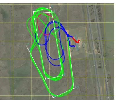
4.9 Photo taken at Canberra Model Aircraft Club. . . 89
4.10 Photo taken at Canberra Model Aircraft Club. . . 89
4.11 Flight path of the plane according to GPS measurements. . . 95
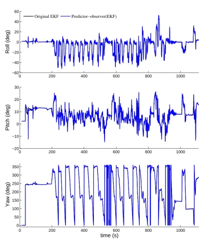
4.12 Estimates of the Euler angles of the plane . . . 96
4.13 North position of the plane provided by GPS versus its prediction . . . . 97
4.14 East position of the plane provided by GPS versus its prediction . . . 98
4.15 North position estimates . . . (default EKF gains are used). . . 99
4.16 East position estimates . . . (default EKF gains are used). . . 101
4.17 North and East position estimates . . . (re-tuned EKF gains are used) . . 101
4.18 North position estimates . . . (high EKF gains are used). . . 102
4.19 East position estimates . . . (high EKF gains are used). . . 102
Introduction
This chapter provides an overview of this thesis by presenting motivations for the subject of this thesis as well as a brief literature review, explaining the problems con-sidered, and listing the main contributions of the thesis. In depth literature reviews and detailed explanations of the contributions are given at the beginning of each chapter.
1.1
Motivation
Many physical systems require the knowledge of their internal states such as their position, orientation, and velocity for various reasons such as effective control, nav-igations, fault detection, path planning, etc. In most practical situations, obtaining a reliable measurement of the internal states of those physical systems directly is not possible and it is necessary to use state estimators. In many applications, par-ticularly in the field of robotics, those internal states naturally lives on Lie groups [17, 32, 40, 71]. For instance, take the attitude estimation problem which is to de-termine the orientation of a rigid body with respect to a known frame of reference [34, 55, 69, 80, 89, 101, 105, 120, 124, 130, 136, 144]. In this case, the orientation of a rigid body is modeled by a 3×3 orthogonal matrix belonging to the Lie group SO(3). Apart from the attitude estimation problem, design of state estimator on Lie groups is also motivated by real world applications such as; attitude estimation on pose es-timation on SE(3) [25, 63, 65, 116, 121, 135], homography estimation on SL(3) [56], and motion estimation of chained systems on nilpotent Lie groups [97] (e.g. front-wheel drive cars or kinematic cars with k trailers). The Special Linear group SL(2)
which arises in some compute vision applications [44, 73, 96], and complex-valued Lie groups and unitary groups arising in multiantenna transceiver techniques, in
sensor array applications in biomedicine, and in machine learning [51, Section 3] are other motivating examples.
Work on state estimation on Lie groups dates back to 1970s, see e.g. the seminal works of Brockett [38, 39] and Willsky [140, 141]. Stochastic filtering methods and deterministic observers are two competing approaches for designing state estimators. Stochastic methods rely on stochastic modeling of the sensor noise and system model uncertainties to design state estimators that are optimal with respect to some metric. Deterministic observers do not require modeling of stochastic noise. Instead, their objective is to guarantee the stability of the estimation error in the noise free condi-tion. There is a rich literature on stochastic state estimation methods on Lie groups (see e.g. [48, 49, 139] as well as [42, Chapters 14 and 15] and the references therein) and their applications to real world problems [44, 46, 66, 98, 104, 105, 114, 126]. Nev-ertheless, this thesis chooses the deterministic setup for modeling and design of state estimators. Hence, in the context of this thesis, the word "state estimator" refers to the "state observer" and we use these two words interchangeably.
Systematic observer design methodologies for deterministic state estimation of in-variant systems ongeneralLie groups have been proposed that lead to strong stability and robustness properties [28, 34, 94]. All of these observer design methodologies require fusing the measurements of both inputs and outputs of systems. In practice, those input and output measurements are nonideal and may be corrupted by sensor biases, sensor sampling, and sensor delays. These effects, if not compensated for properly, might lead to poor performance of the observers or even cause instability [22, 53, 74, 76, 100, 106, 109, 117, 125].
The effects of nonideal measurements are more significant in robotics applica-tions involving low cost sensor suites. For instance, low cost MEMS1 gyros usually exhibit a significant measurement bias which should be compensated to obtain re-liable estimations of attitude [101, 116, 136]. Commercial GPS units usually exhibit a significant measurement delay that can be as large as hundreds of milliseconds. Those GPS units normally provide low sampling rates (less than 5 Hz) [58, 88]. The effects of these delays and sampling are very significant in commercial UAVs where onboard navigation algorithms normally run as fast as 50-200 Hz [4]. Similar de-lay and sampling effects are present in indoor flight environments where the pose
data provided by devices such as VICON or OptiTrack are available to the onboard navigation system of UAVs with variable delays and sampling rates due to the com-munication channel from those sensors to the UAV. In satellite attitude estimation applications, sampling effects are present where high accuracy output sensors such as star trackers or earth sensors provide measurements at low sampling rates (0.5 to 10 Hz) [105].
For the special problem of attitude estimation on SO(3), observers are available in the literature that adaptively compensate for the gyro bias [101, 116, 136]2. A similar observer is designed for adaptively estimating both the linear and angular veloc-ity biases in the pose estimation problem on SE(3) [135]. This naturally raises the problem of generalizing the concurrent state and input bias estimation to invariant systems ongeneralLie groups. This problem is investigated in Chapter 2 where a sys-tematic observer design methodology is proposed that unifies the SO(3) and SE(3)
examples into a single framework that applies to any invariant kinematic system on a Lie group.
A particular focus of this thesis is state estimation with output measurement de-lays and sampling. This problem attracted our attention when a group of autopilot developers at Canberra UAV [7] reported occasional oscillations leading to instability of the popular attitude observer of [101]. In his talk at the Australian National Uni-versity, Andrew Tridgell3 [131] presented flight tests showing that the geometric ob-server of [101] is prone to instability if accelerometer measurements are aided by GPS velocity measurements. Reconstructing the flight test using a software-in-the-loop system, he concluded that the GPS delay and sampling effects are the main causes of the instability when the UAVs perform high acceleration maneuvers. This is the main motivation for consideration of the output measurement delay and sampling problems in Chapters 3 and 4, respectively. We propose predictors to compensate for the delay and sampling effects for invariant systems on general Lie groups. The resulting theory is not only applicable to the GPS delay problem discussed above, it is also applicable to lots of similar practical problems such as the time varying sampling and delay problem of VICON or OptiTrack in indoor flight environments, the sampling and delay problem of visual navigation systems, and attitude estima-2This observer is commonly known as DCM (Direction Cosine Matrix) amongst UAV enthusiasts
and the robotics community [8, 12].
tion using star sensors with low sampling rates. Through a close collaboration with Andrew Tridgell’s team at Canberra UAV and 3DRobotics [1], we implemented the proposed predictors into the embedded autopilot system of model UAVs and verified their performance in real flight tests. The main strength of this thesis is to provide a balance between a very high level of abstraction of the developed theoretical results (by providing theories applicable to systems on general Lie groups) and justifying those theories by presenting real world applications and experimental verifications with real UAVs.
1.2
A first literature review
Systematic observer design methodologies for invariant systems on general Lie groups have been proposed that lead to strong stability and robustness properties. Partic-ularly, Bonnabel et al. [33–35] consider observers which consist of a copy of the system and a correction term, along with a constructive method to find suitable symmetry-preserving correction terms. The construction utilizes the invariance of the system and the moving frame method, leading to local convergence properties of the observers. Also, [28] extends those constructive methods in order to apply them to a wider class of systems on Lie groups. This leads to development of a so-called Invariant Extended Kalman Filtering approach with provable local stability properties. Methods proposed in [92–94] to achieve almost globally convergent ob-servers. A key aspect of the design approach proposed in [92–94] is the use of the invariance properties of the system to ensure that the error dynamics are globally defined and are autonomous. This leads to a straight forward stability analysis and excellent performance in practice. More recent extensions to early work in this area was the consideration of output measurements where a partial state measurement is generated by an action of the Lie group on a homogeneous output space [33– 35, 92, 93, 102]. Also, [123, 143] develop a rigorous theory for designing minimum energy observers on Lie groups with near optimal performance. Recently, [69, 70] proposed state estimation methods on the specific Lie groups SO(3)and SE(3)based on the Lagrange–d’Alembert principle.
methods strongly depend on particular properties of the specific Lie groups SO(3)
or SE(3)and do not directly generalize to general Lie groups.
Deterministic state estimation for systems onRnwith sampled and delayed mea-surements is a classical problem that has been extensively studied and many results with strong stability proofs are currently available [16, 18, 19, 30, 41, 41, 53, 74– 76, 134]. Nevertheless, no such results are available (prior to this thesis) for systems on general Lie groups. The only available publications in this are [24] and [58] that consider the special case of attitude estimation.
In this thesis, we consider the state estimation for invariant systems on general Lie groups where input measurement bias, output measurement delay and sampling are present. In the following, we further describe these problems. In depth literature reviews and detailed explanations of each problem are given at the beginning of the associated chapter.
1.3
Problems considered
We consider three classes of nonideal measurements; input measurement corrupted by unknown bias, output measurement with delay, and output measurement with sampling.
1.3.1 Unknown input measurement bias
1.3.2 Output measurement delay
In many practical scenarios, measurements of the outputs of the system are usually available to the user with some delay (due to various reasons including physical properties of sensors or the environment, slow transients, internal signal processing of sensors, extensive filtering of sensor measurements for noise reduction, and com-munication delays from sensors to processing units) while the inputs are measured without significant delays. For example, in the velocity aided attitude estimation problem, measurements of the linear velocity (output) provided by commercial GPS units are usually delayed with respect to the actual velocity of the vehicle. In contrast, measurements of the vehicle’s angular velocity and linear acceleration provided by an onboard IMU are almost instantaneous. In Chapter 3, we provide anobserver-predictor methodology to cope with the output measurement delay for invariant systems on general Lie groups. In this method, the observer takes the delayed measurements and provides estimates of the delayed state. We propose predictors that take the estimates of the delayed state, compensate for the delay, and provide predictions of the current state.
1.3.3 Output measurement sampling
we investigate the problem of state estimation for invariant systems on general Lie groups where the measurements of outputs are sampled and delayed. We propose a cascade predictor-observer approach in which the predictor takes the sampled and delayed output measurements and provides predictions of the current outputs. The predicted outputs are then fed into an observer or filter to estimate the system states. Compared to the method proposed in Chapter 3, the method of Chapter 4 provides stronger tools for state estimation by eliminating both output sampling and delay effects. Nevertheless, it extensively relies on symmetries of the output maps of the system and hence is less flexible than the method of Chapter 3 in dealing with diverse classes of outputs.
1.4
Thesis contributions
The main theoretical contribution of the thesis is to effectively employ the underlying symmetries of the system dynamics and output maps in order to propose methodolo-gies to cope with the problems discussed in the previous section. In the following, we briefly discuss the main contributions of the thesis. More detailed discussions about the contributions of each chapter is given in the introductory part and the conclusion of each chapter.
• We tackle the problem of state estimation for systems on general matrix Lie groups when measurements of system outputs are delayed. This problem is investigated in Chapter 3. We propose an observer-predictor methodology for invariant systems on Lie groups. Given an observer or filter that has desired stability properties when the system outputs are delay-free, we propose an observer-predictor methodology that preserves those stability properties when the system outputs are delayed. We design dynamic predictors that use the delayed estimates from the observers together with the current inputs in or-der to predict the current state of the system (Theorems 3.3.3 and 3.3.4). The proposed predictors are computationally very cheap and demonstrate excel-lent robustness properties, making them ideal for embedded implementation on low cost robotics applications. The results of Chapter 3 are presented in [82, 84].
• We consider the state estimation problem for invariant systems on Lie groups where sampled and delayed output measurements are available. This problem is investigated in Chapter 4. We propose a cascade predictor-observer approach in which the predictor takes the sampled and delayed output measurements and provides predictions of the current outputs. The predicted outputs are then fed into an observer or filter to estimate the system states. We prove that in noise free conditions, the current prediction of the output is indeed equal to the actual ideal output, independent of the sampling rate and delay associated with the output measurement (Theorem 4.4.1). This is a very strong result which enables application of the developed predictors in a wide range of real world applications involving multi rate sensors with possibly different and even time-varying delays. A preliminary version of the results of Chapter 4 are presented in [83].
proposed predictors by presenting real flight tests with model UAVs (Section 4.6.1). We further illustrate the advantages of the proposed method over avail-able state-of-the-art estimation approaches by offline processing of sensor data using post-processing tools of the ArduPilot system (Section 4.6.4).
1.5
Notations and definitions
We use the following notations throughout this thesis. Let Gbe a finite-dimensional real connected Lie group with associated Lie algebra g. Denote the identity element of G by I. Left (resp. right) multiplication of X ∈ G by S ∈ G is denoted by LSX = SX (resp. RSX = XS). The Lie algebragcan be identified with the tangent
space at the identity element of the Lie group, i.e. g ∼= TIG. For any u ∈ g, one
can obtain a tangent vector at S ∈ G by left (resp. right) translation of u denoted by S[u] := TILS[u] ∈ TSG (resp. [u]S := TIRS[u] ∈ TSG). The element inside the
brackets [.] denotes the vector on which a linear mapping (here the tangent map TILS: g → TSG or TIRS: g → TSG) acts. For convenience, we omit the notation [.]
if there is no risk of confusion. The adjoint map at the point S ∈ G is denoted by AdS: g → g and is defined by AdS[u] := S[u]S−1 = TSRS−1[TILS[u]] = TSRS−1 ◦
TILS[u] where ◦ denotes the composition of two maps. Choose an inner product
hh., .iiongand denote the corresponding induced norm ongbyk.k. Denote byh., .ir S
(resp. h., .il
S) a right-invariant (resp. left-invariant) Riemannian metric at a point S
induced by hh., .ii using right (resp. left) translation of the Lie algebra g. Denote the corresponding induced right-invariant (resp. left-invariant) norm on TSGby|.|rS
(resp. |.|l
S). Denote the geodesic distance with respect to (w.r.t.) h., .ir (resp. h., .il)
between the points S and X by dr(S,X) (resp. dl(S,X)). For a finite-dimensional
definite and it is called symmetric ifH∗ is symmetric. Positive definite cost functions on manifolds are also used in the thesis and should not be mistaken with positive definite linear maps. The notations σ(AdS) and σ(AdS), respectively, denotes the
smallest and the largest singular value of the adjoint map w.r.t. the normk.k, defined byσ(AdS):= min
v∈g,kvk=1
kAdSvkandσ(AdS):= max v∈g,kvk=1
kAdSvk, respectively. For a
matrix A ∈ Rm×m, the notations
σ(A), σ(A), and cond(A), respectively, denote the smallest singular value, the largest singular value, and the condition number of that matrix (with respect to the Euclidean norm onRm). We say the trajectorya(t)∈R+
converges to zero and denote a(t)→0 if lim
t→+∞a(t) = 0. We writea(t) exp
−→0 and we saya(t)converges exponentially to zero if there exist positive constantscandαsuch that a(t)≤cexp(−αt)for allt≥0.
The following standard definitions are used thought the thesis [36, 61, 90]. The group actionh: G×M→ M is calledtransitiveif there exists ˚y ∈ Msuch that every y ∈ M satisfies y = h(X, ˚y)for some X ∈ G. The space M is called a homogeneous space ofGif there exists a transitive action ofGon M. The Lie groupGhas afaithful representationas a finite-dimensional matrix Lie group if there exist a positive integer mand an injective Lie group homomorphismΦ: G→GL(m)into the group GL(m)
Input Bias Estimation for Invariant
Systems on Lie Groups with
Homogeneous Outputs
This chapter provides a new observer design methodology for invariant systems whose state evolves on a Lie group with outputs in a collection of related homo-geneous spaces and where the measurement of system input is corrupted by an unknown constant bias. The key contribution of the Chapter is to study the com-bined state and input bias estimation problem in the general setting of Lie groups, a question for which only case studies of specific Lie groups are available in prior liter-ature. We show that any candidate observer (with the same state space dimension as the observed system) results in non-autonomous error dynamics, except in the trivial case where the Lie group is Abelian. This precludes the application of the standard non-linear observer design methodologies available in the literature and leads us to propose a new design methodology based on employing invariant cost functions and general gain mappings. We provide a rigorous and general stability analysis for the case where the underlying Lie group allows a faithful matrix representation. We demonstrate our theory in the example of rigid body pose estimation and show that the proposed approach unifies two competing pose observers published in prior literature. The contributions presented in this chapter are published in [85–87].
2.1
Related work
Many mechanical systems carry a natural symmetry or invariance structure ex-pressed as invariance properties of their dynamical models under transformation by a symmetry group. For totally symmetric kinematic systems, the system can be lifted to an invariant system on the symmetry group [102]. Work in this area is motivated by applications in analytical mechanics, robotics and geometric control of mechanical systems [17, 32, 40, 71, 105]. Systematic observer design methodologies for deterministic state estimation of invariant systems on general Lie groups have been proposed that lead to strong stability and robustness properties [28, 34, 94]. All asymptotically stable observer designs for kinematic systems on Lie groups depend on a measurement of system input [28, 33, 68, 94, 102, 123, 143]. In practice, mea-surements of system input are often corrupted by an unknown bias that must be estimated and compensated to achieve good observer error performance. The spe-cific cases of attitude estimation on SO(3) and pose estimation on SE(3)have been studied independently, and methods have been proposed for the concurrent estima-tion of state and input measurement bias [101, 135, 136]. These methods strongly depend on particular properties of the specific Lie groups SO(3) or SE(3) and do not directly generalize to general Lie groups. To our knowledge, there is no existing work on combined state and input bias estimation for general classes of invariant systems.
result explains why the previous general observer design methodologies for the bias-free case do not apply and why the special cases considered in prior works [65, 135] do not naturally lead to a general theory.
We go on to show that, despite the nonlinear and non-autonomous nature of the error dynamics, there is a natural choice of observer for which we can prove exponential stability of the error dynamics (Theorems 2.4.1 and 2.4.3). The approach taken employs a general gain mapping applied to the differential of a cost function rather than the more restrictive gradient-like innovations used in prior work [92–94]. We also propose a systematic method for construction of invariant cost functions based on lifting costs defined on the homogeneous output spaces (Proposition 2.5.1). To demonstrate the generality of the proposed approach we consider the problem of rigid body pose estimation using landmark measurements when the measurements of linear and angular velocity are corrupted by constant unknown biases. We show that for specific choices of gain mappings the resulting observer specializes to either the gradient-like observer of [65] or the non-gradient pose estimator proposed in [135], unifying these two state-of-the-art application papers in a single framework that applies to any invariant kinematic system on a Lie group.
The Chapter is organized as follows. We formulate the problem in Section 2.2. A standard estimation error is defined and autonomy of the resulting error dynamics is investigated in Section 2.3. We introduce the proposed observer in Section 2.4 and investigate the stability of observer error dynamics. Section 2.5 is devoted to the systematic construction of invariant cost functions. A gradient based observer design example in Section 2.6 and a non-gradient example in Section 2.7 followed by brief conclusions in Section 2.8 complete the Chapter.
2.2
Problem Formulation
We consider a class of left invariant systems onGgiven by ˙
whereu∈ gis the system input andX∈ Gis the state1. We assume thatu: R+ →g is continuous and hence a unique solution for (2.1) exists for allt ≥ t0 [72]. In most kinematic mechanical systems,umodels the velocity of physical objects. Hence, it is reasonable to assume thatuis bounded and continuous.
Let Mi, i = 1, . . . ,n denote a collection of n homogeneous spaces of G, termed
output spaces. Denote the outputs of system (2.1) by yi ∈ Mi. Suppose each output
provides a partial measurement ofX via
yi = hi(X, ˚yi) (2.2)
where ˚yi ∈ Mi is the constant (with respect to time) reference output associated
with yi and hi is a right action of G on Mi, i.e. hi(I,yi) = yi and hi(XS,yi) =
hi(S,hi(X,yi)) for all yi ∈ Mi and all X,S ∈ G2. Although the ideas presented in
this chapter are based on the left invariant dynamics with right output actions, they can easily be modified for right invariant systems with left output actions as was done for instance in [94]. To simplify the notation, we define the combined output y := (y1, . . . ,yn), the combined reference output ˚y := (y˚1, . . . , ˚yn), and the combined
right action h(X, ˚y):= (h1(X, ˚y1), . . . ,hn(X, ˚yn)). The combined output ybelongs to
the orbit of G acting on the product space M1×M2×. . .×Mn containing ˚y, that
is M := {y ∈ M1×M2×. . .×Mn| y = h(X, ˚y), X ∈ G} ⊂ M1×M2×. . .×Mn.
Note that the combined actionhofGdefined above is transitive on M. Hence, Mis a homogeneous space ofGwhileM1×M2×. . .×Mnis not necessarily a homogeneous
space ofG[91].
We assume that measurements of the system input are corrupted by a constant unknown additive bias. That is
uy= u+b (2.3)
1In Chapters 3 and 4 where we consider left-invariant, right-invariant, and mixed-invariant systems,
we denote the states of those systems byXl,Xr, andXm, respectively. Since in this chapter we only talk
about the left-invariant system 2.1, for convenience, we omit the subscriptland simplify the notation toX.
2In Chapters 3 and 4 where we consider both right and left output actions, we denote the associated
actions byhr andhl, respectively. Since in this chapter we only talk about the right output action 2.2,
where uy ∈ g is the measurement of u and b ∈ g is the unknown bias. In practice,
bias is slowly time-varying but it is common to assume thatbis constant for observer design and analysis.
We investigate the observer design problem for concurrent estimation of X and b. The observer should be implementable based on sensor measurements. This is important since the actual state X ∈ Gand the actual input u ∈ g are not available for measurement and only the partial measurementsy1, . . . ,yn and the biased input
uy are directly measured. We consider the following general class of implementable
observers with the same state space dimension as the observed system. ˙ˆ
X=γ(X,ˆ y, ˚y, ˆb,uy,t) (2.4a)
˙ˆ
b=β(X,ˆ y, ˚y, ˆb,uy,t) (2.4b)
where ˆXand ˆbare the estimates ofXandb, respectively, andγ: G×M×M×g×g×
R → TG andβ: G×M×M×g×g×R → gare parameterized vector fields on G andg, respectively. Note that ˆX,y, ˚y, ˆb,uyandtare all available for implementation of
the observer in practical scenarios. We refer to (2.4a) and (2.4b) as thegroup estimator and thebias estimator, respectively.
Example 2.2.1(Attitude Estimation on SO(3)). Attitude estimation is a classical problem which is still a popular research topic [34, 37, 55, 65, 69, 80, 101, 105, 108, 116, 120, 121, 124, 133, 136, 144]. The attitude of a rigid body can be identified by a rotation matrix belonging to the Lie group R ∈ SO(3)representing the rotation from body-fixed frame {B} to the inertial frame{A}. The Lie algebra of SO(3)is identified by the set of skew-symmetric 3×3matrices with zero trace denoted byso(3). The attitude kinematics on SO(3)is given by
˙
R(t) =R(t)Ω(t) (2.5)
where Ω ∈ so(3) represents the angular velocity of {B}with respect to {A}expressed in {B}. Assume that partial attitude information is provided by vectorial measurements yi in
{B}. Such a measurement can be provided by an on-board sensor system such as a 3-axis magnetometer. We recall that in most practical cases, the constant inertial directiony˚i ∈ {A}
by
yi(t) =R(t)>y˚i. (2.6)
The vectors yi andy˚i are normalized to have unit norms such that the measured output lives
in S2. The output map (2.6) defines a right action of SO(3)on the homogeneous output space Mi ∼=S2by hi(R, ˚yi):=R>y˚i.
The angular velocity measured by rate gyros is usually disturbed by additive unknown bias such that
Ωy(t) =Ω(t) +b (2.7)
where Ωy is the measured angular velocity and b denotes the unknown constant bias. The
attitude estimation problem is to use the measurementsΩyand yi, i=1, . . . ,n together with
a-priori knowledge y˚i, i = 1, . . . ,n in order to estimate the attitude matrix R and the gyro
bias b.
Example 2.2.2 (Pose Estimation on SE(3)). Estimating the position and attitude of a rigid body has been investigated by a range of authors during the past decades, see, e.g.,
[25, 65, 116, 135, 138]. The full 6-DOF pose kinematics of a rigid body can be modeled as an invariant system on the special Euclidean group SE(3) [94, 116, 135, 138]. The Lie group SE(3) has a representation as a semi-direct product of SO(3) and R3 given by SE(3) =
{(R,p)| R ∈ SO(3), p ∈ R3}[36]. Consider the group multiplication on SE(3)given by R(S,q)(R,p) = L(R,p)(S,q) = (RS,p+Rq) for any(R,p),(S,q) ∈ SE(3). The identity
element of SE(3)is represented by(I3×3, 03)and the inverse of an element(R,p)∈ SE(3) is given by (R,p)−1 = (R>,−R>p). The Lie algebra of SE(3) is identified with se(3) = {(Ω,V)|Ω∈so(3), V∈ R3}.
Let R represent the attitude matrix of a rigid body, as was discussed in Example 2.2.1,
and suppose that p represents the position of the rigid body with respect to the inertial frame and expressed in the inertial frame. The left-invariant kinematics of the rigid body on SE(3)
is formulated as
(R, ˙˙ p) =TIL(R,p)(Ω,V) = (RΩ,RV) (2.8)
respect to the inertial frame expressed in the body-fixed frame. Here, the group element is X= (R,p)∈ SE(3)and the system input is u= (Ω,V)∈se(3). Denote the measurement of the system input by (Ωy,Vy) ∈ se(3) and assume that it is corrupted by an unknown
constant bias (bω,bv) ∈ se(3) such that (Ωy,Vy) = (Ω+bω,V+bv). Suppose that
positions of n points with respect to the body-fixed frame are measured by on-board sensors
and denote these measurements by y1, . . . ,yn ∈R3. Denote the positions of these points with
respect to the inertial frame byy˚i, i =1, . . . ,n ∈R3 and assume these positions are known
and constant. The output model for such a set of measurements is given by
yi =hi((R,p), ˚y1) =R>y˚i−R>p, i=1, . . . ,n (2.9)
where hi is a right action of SE(3) on the homogeneous output space Mi := R3. A
practi-cal example of measurements modeled by (2.9) is vision based landmark readings where the
landmarks are fixed in the inertial frame, leading to constanty˚i, i=1, . . . ,n [135]. The pose
estimation problem is to estimate R and p together with the input biases bω and bv.
2.3
Error Definition and Autonomy of Error Dynamics
We consider the following right-invariant group error,
E= XXˆ −1∈ G, (2.10)
as was proposed in [94, 102]. The above error resembles the usual error ˆx−x used in classical observer theory when ˆx,xbelong to a vector space. We also consider the following bias estimation error
˜
b=bˆ−b∈g. (2.11)
non-autonomous error dynamics for general Lie groups, and it can only produce au-tonomous error dynamics for Abelian Lie groups. To prove this result, we note that the observer (2.4) can be rewritten into the form
˙ˆ
X=Xˆ[uy−bˆ]−αy˚(X,ˆ y, ˆb,uy,t), (2.12a)
˙ˆ
b=βy˚(X,ˆ y, ˆb,uy,t), (2.12b)
whereαy˚: G×M×g×g×R→TGandβy˚: G×M×g×g×R→gare parameter-ized vector fields on G andg, respectively, and ˚y is now interpreted as a parameter forαy˚and βy˚.
Theorem 2.3.1. Consider the observer (2.12) for the system (2.1)-(2.3). The error dynamics
(E, ˙˜˙ b)is autonomous if and only if all of the following conditions hold; (a) αy˚ andβy˚do not depend onb, uˆ yand t.
(b) The vector fieldαy˚is right equivariant in the sense that TXˆRZαy˚(X,ˆ y) =αy˚(XZ,ˆ h(Z,y)) for allX,ˆ Z∈G and all y∈ M.
(c) The vector fieldβy˚ is right invariant in the sense thatβy˚(X,ˆ y) = βy˚(XZ,ˆ h(Z,y))for allX,ˆ Z∈G and all y ∈ M.
(d) For all Z∈G the adjoint map AdZ: g→gis the identity map.
Proof: In view of (2.1) and (2.12), differentiating E = XXˆ −1 and ˜b= bˆ−b with respect to time yields
˙
E= −TXˆRX−1αy˚(X,ˆ y, ˆb,uy,t)−TIREAdXˆb˜ (2.13a) ˙˜
b= βy˚(X,ˆ y, ˆb,uy,t). (2.13b)
If the conditions (a) to (d) of the Theorem hold, the error dynamics will be simplified to
˙
E=−αy˚(XXˆ −1,h(X−1,y))−TIREb˜=−αy˚(E, ˚y)−TIREb,˜ (2.14a)
˙˜
b= βy˚(XXˆ −1,h(X−1,y)) = βy˚(E, ˚y), (2.14b)
Conversely, assume that the error dynamics (2.13) are autonomous. Then there exist functionsFy˚: G×g→TGandHy˚: G×g→gsuch that for allX, ˆX∈G,y∈ M, ˆ
b,uy∈g,
˙
E=−TXˆRX−1αy˚(X,ˆ y, ˆb,uy,t)−TIREAdXˆb˜ =Fy˚(E, ˜b) (2.15a) ˙˜
b=βy˚(X,ˆ y, ˆb,uy,t) =Hy˚(E, ˜b). (2.15b)
It immediately follows that αy˚ and βy˚ are independent of uy and t. Moreover,
since the error E = XXˆ −1 is invariant with respect to the transformation (X,ˆ X) 7→
(XZ,ˆ XZ) for all Z ∈ G and the error ˜b = bˆ −b is invariant with respect to the transformation(b,ˆ b)7→ (bˆ+d,b+d)for alld ∈g, we have
−TXˆRX−1αy˚(X,ˆ y, ˆb)−TIREAdXˆb˜ = Fy˚(E, ˜b) (2.16a)
=−TXZˆ R(XZ)−1αy˚(XZ,ˆ h(Z,y), ˆb+d)−TIREAdXZˆ b,˜ βy˚(X,ˆ y, ˆb) =Hy˚(E, ˜b) =βy˚(XZ,ˆ h(Z,y), ˆb+d). (2.16b) From (2.16b) it follows thatβy˚is independent of ˆbsince the right hand side of (2.16b) depends on d while the left hand side is independent of this variable. This estab-lishes condition (a) for βy˚. It also follows that βy˚ satisfies the invariance condition βy˚(X,ˆ y) =βy˚(XZ,ˆ h(Z,y))(condition (c) of the Theorem). We can rearrange (2.16a) to obtain
−TXˆRX−1αy˚(X,ˆ y, ˆb)−TIREAdXˆb˜+TIREAdXZˆ b˜ = −TXZˆ R(XZ)−1αy˚(XZ,ˆ h(Z,y), ˆb+d). (2.17) The right hand side of (2.17) is a function of d while the left hand side is not. This implies that αy˚ is independent of ˆb (establishing condition (a) forαy˚). We can then rearrange (2.17) again to obtain
−TXˆRX−1αy˚(X,ˆ y) +TXZˆ R(XZ)−1αy˚(XZ,ˆ h(Z,y)) =TIREAdXˆb˜ −TIREAdXZˆ b. (2.18)˜
andTIREAdXZˆ b˜ = TIREAdXˆb˜ for all ˜b∈ gand all E, ˆX,Z∈ G. These equations im-ply TXˆRZαy˚(X,ˆ y) = αy˚(XZ,ˆ h(Z,y))and AdZb˜ = b˜ to obtain conditions (b) and (d)
imposed in the theorem, respectively. This completes the proof.
Remark 2.3.2. If G is a real, finite-dimensional, connected Lie group then condition (d) of
Theorem 2.3.1 implies that G is Abelian [90, Proposition 1.91]. By the structure theorem for connected Abelian Lie groups [36, Proposition III.6.4.11], this means that G is isomorphic to a product Rn×(S1)m whereRn is additive and(S1)m denotes the m-dimensional torus.
This class of Lie groups is far more specific than the Lie groups that are encountered in many practical applications. For robotics applications, the Lie groups typically considered are
SO(3) and SE(3) both of which are non-Abelian. Theorem 2.3.1 in particular implies that all implementable geometric bias estimators on SO(3) and SE(3)proposed in the literature produce non-autonomous standard error dynamics (see [101] and [135]).
2.4
Observer Design and Analysis
We propose the following implementable group estimator, ˙ˆ
X= Xˆ[uy−bˆ]−Ky˚(X,ˆ y, ˆb,uy,t)[D1φy˚(X,ˆ y)], (2.19)
with ˆX(t0) = Xˆ0 where φy˚: G×M → R+ is a C2 cost function, D1φ˚y(X,ˆ y) ∈ TX∗ˆG denotes the differential ofφy˚i with respect to its first argument evaluated at the point
(X,ˆ y) and Ky˚(X,ˆ y, ˆb,uy,t) is a linear gain mapping from TX∗ˆG to TXˆG. Note that ˚y is considered to be a parameter for Ky˚ andφy˚. The above group estimator matches the structure of (2.12a) where the innovation αy˚ is generated by applying the gain mapping Ky˚ to the differential D1φy˚. By Theorem 2.3.1, we already know that the above estimator cannot produce autonomous error dynamics for a general Lie group. Hence, there is no reason to omit the arguments ˆb,uy andt of the gain mapping. If
the gain mapping Ky˚ is symmetric positive definite and independent of ˆb,uy andt,
We consider the following bias estimator, ˙ˆ
b=Γ◦TIL∗Xˆ[D1φy˚(X,ˆ y)], bˆ(t0) =bˆ0, (2.20)
where TIL∗Xˆ: TX∗ˆG→ g∗ is the dual of the mapTILXˆ (see Section 1.5) andΓ: g∗ → g is a constant gain mapping.
We will require the following assumptions for statement of results.
(A1) The Lie group G has a faithful representation as a finite-dimensional matrix Lie group. That is, there exist a positive integer mand an injective Lie group homomorphism Φ : G → GL(m) into the group GL(m) of invertible m×m matrices. Note thatΦ(G)is a matrix subgroup of GL(m).
(A2) [boundedness conditions] Φ(X), Φ(X)−1, u and K(X,ˆ y, ˆb,uy,t) are bounded
along the system trajectories.
(A3) [differentiability conditions] ˙u(t), the first differentials ofhi(X, ˚yi)andK(X,ˆ y, ˆb,uy,t),
as well as the first and the second differential3of φ(X,ˆ y)with respect to all of their arguments are bounded along the system trajectories.
Theorem 2.4.1. Consider the observer (2.19)-(2.20) for the system (2.1)-(2.3). Suppose that assumptions (A1), (A2) and (A3) hold. Assume moreover that the gain mappings K and Γ, and the cost functionφsatisfy the following properties;
(a) The gain mapping Ky˚:TX∗ˆG → TXˆG is uniformly positive definite (not necessarily symmetric). That is, there exist positive constants k and k and a continues vector norm |.| on TX∗ˆG such that for all v∗ ∈ TX∗ˆG we have k|v∗|2 ≤ v∗[K
˚
y(X,ˆ y, ˆb,uy,t)[v∗]]≤
k|v∗|2.
(b) The gain mappingΓ:g∗→gis symmetric positive definite.
(c) The costφy˚ is right invariant, that is φy˚(XZ,ˆ h(Z,y)) = φy˚(X,ˆ y)for all X,ˆ Z ∈ G and all y∈ M.
(d) The costφy˚(., ˚y): G → R+, E 7→ φy˚(E, ˚y)is locally positive definite around E = I and it has an isolated critical point at E= I.
3Second differential ofφis either in the sense of embedding the Lie group intoRm×mor in the sense
Then the error dynamics(E, ˙˜˙ b)is uniformly locally asymptotically stable at(I, 0).
Proof: The following result is used in the development later in this proof.
Lemma 2.4.2. Letφy˚: G×M →R+be a right-invariant cost function in the sense defined in part (c) of Theorem 2.4.1. Then we have
D1φy˚(X,ˆ y) =TXˆR∗X−1[D1φy˚(E, ˚y)] (2.21) D1φy˚(E, ˚y) =D1φy˚(X,ˆ y)◦TERX (2.22)
Proof of Lemma 2.4.2: The right-invariance property of φy˚ implies φy˚(X,ˆ y) =φy˚◦ RX−1(X,ˆ y). Differentiating both sides in an arbitrary direction v ∈ TXˆG and using
the chain rule we obtain D1φy˚(X,ˆ y)[v] = D1φy˚(E, ˚y)◦TXˆRX−1[v]. Since vis arbitrary
and by using the duality we have D1φy˚(X,ˆ y) = TXˆR∗X−1[D1φy˚(E, ˚y)] which proves (2.21). Applying (TXˆRX−1)−1 = TERX from the right to both sides of D1φy˚(X,ˆ y) = D1φy˚(E, ˚y)◦TXˆRX−1 yields (2.22). This completes the proof of Lemma 2.4.2.
For simplicity, we denote Ky˚(X,ˆ y, ˆb,uy,t)by Ky˚(.). Considering (2.1), (2.3), and (2.19), the group error dynamics are given by
˙
E=XX˙ˆ −1+XˆX˙−1=T ˆ
XRX−1◦TILXˆ[u]−TXˆRX−1◦TILXˆ[b˜]
−TXˆRX−1◦Ky˚(.)[D1φy˚(X,ˆ y)]−TXˆRX−1◦TILXˆ[u]
=−TXˆRX−1◦TILXˆ[b˜]−TXˆRX−1◦Ky˚(.)◦TXˆRX∗−1[D1φy˚(E, ˚y)], (2.23)
where Eis as in (2.10) and (2.21) is used in the last line of (2.23). Now, consider the candidate Lyapunov function,
L(E, ˜b) =φy˚(E, ˚y) + 1 2Γ
−1[b˜][b˜]. (2.24)
The Lyapunov candidate is at least locally positive definite due to conditions (b) and (d). The time derivative ofLis given by
˙
Recalling that ˙˜b=b˙ˆ and substituting ˙Eform (2.23) in (2.25), we obtain ˙
L(E, ˜b) =−D1φy˚(E, ˚y)[TXˆRX−1◦Ky˚(.)◦TXˆR∗X−1[D1φy˚(E, ˚y)]]
−D1φy˚(E, ˚y)[TXˆRX−1◦TILXˆ[b˜]] +Γ−1[b˙ˆ][b˜]. (2.26)
Using (2.22), we conclude ˙
L(E, ˜b) =−D1φy˚(E, ˚y)[TXˆRX−1◦Ky˚(.)◦TXˆR∗X−1[D1φy˚(E, ˚y)]] −D1φy˚(X,ˆ y)◦TERX◦TXˆRX−1◦TILXˆ[b˜] +Γ−1[b˙ˆ][b˜]
=−D1φy˚(E, ˚y)[TXˆRX−1◦Ky˚(.)◦TXˆR∗X−1[D1φy˚(E, ˚y)]]
−D1φy˚(X,ˆ y)◦TILXˆ[b˜] +Γ−1[b˙ˆ][b˜]. (2.27)
Now, replacing ˙ˆbwith (2.20) we obtain ˙
L(E, ˜b) =−D1φy˚(E, ˚y)[TXˆRX−1◦Ky˚(.)◦TXˆR∗X−1[D1φy˚(E, ˚y)]]
−D1φy˚(X,yˆ )◦TILXˆ[b˜]+Γ−1◦Γ◦TIL∗Xˆ◦D1φy˚(X,ˆ y)[b˜]. (2.28)
Duality implies D1φy˚(X,ˆ y)◦TILXˆ =TIL∗Xˆ ◦D1φy˚(X,ˆ y)and (2.28) simplifies to ˙
L(E, ˜b) =−D1φy˚(E, ˚y)[TXˆRX−1◦Ky˚(.)◦TXˆRX∗−1[D1φy˚(E, ˚y)]]. (2.29)
Since Ky˚(.) is assumed to be positive definite and the map TXˆRX−1 is full rank, the
map TXˆRX−1 ◦Ky˚(.)◦TXˆR∗
X−1 is positive definite. This implies that ˙L(E, ˜b) ≤ 0 and
hence the Lyapunov function is non-increasing along the system trajectories. We adopt the proof of [78, Theorem 4.8] to prove uniformly local stability of error dynam-ics. Recalling assumption (A1), distance to the identity element of G is denoted by d(.)and is induced by Frobenius norm on Φ(G)⊂Rm×m via d(E):=kId−Φ(E)kF where Id is the identity matrix. Define the compound error ˜x:= (E, ˜b)∈ G×gand obtain the distance of ˜xto (I, 0)byl(x˜)2 := d(E)2+kb˜k2
g wherek.kgdenotes a norm
on g. Using assumption (d), there exist a ball Br := {E ∈ G : d(E) ≤ r}such that
φy˚(., ˚y)is positive definite onBr. ConsequentlyL(x˜)is positive definite on ¯Br:={x˜∈
G×g : l(x˜)≤ r}. Choosec <minl(x˜)=rL(x˜)and defineΩc := {x˜ ∈ B¯r| L(x˜)≤ c}.
other hand, sinceL(x˜)is positive definite onΩc ⊂ B¯r, there exist classK functions
η1 and η2 such that η1(l(x˜)) ≤ L(x˜) ≤ η2(l(x˜)) for all ˜x ∈ Ωc [78, Lemma 4.3].
Consequently, we have l(x˜(t))≤ η−11(L(x˜(t)))≤ η1−1(L(x˜(t0)))≤ η1−1(η2(l(x˜(t0)))) which implies l(x˜(t)) ≤ η1−1◦η2(l(x˜(t0))). Since η1−1◦η2 is a class K function (by [78, Lemma 4.2]), the equilibrium point ˜x = (I, 0) is uniformly stable for all initial conditions starting in Ωc [78, Lemma 4.5]. Moreover, the error E is bounded by
d(E(t))≤l(x˜(t))≤η1−1(L(x˜(t0)))≤η−11(c)for such initial conditions.
Boundedness of ˜x(t)implies thatE(t)and ˜b(t)are bounded with respect tod(.)
and k.kg, respectively. Differentiating (2.29) with respect to time and considering
the boundedness of (E(t), ˜b(t)) together with assumptions (A2) and (A3), one can conclude that ¨L(t) is bounded and hence ˙L(t) is uniformly continuous. By invok-ing Barbalat’s lemma we conclude that ˙L(t) → 0. This together with condition (a) implies that D1φy˚(E(t), ˚y)→ 0. Sinceφy˚(E,I)has an isolated critical point atE = I, there exist a ball Bc¯ ⊂ G such that E = I is the only point in Bc¯ where D1φy˚(., ˚y) is zero. We proved before that E(t) ∈ Bη−1
1 (c) for all initial conditions starting in
Ωc. Choosing c < min(η1(c¯), minl(x˜)=rL(x˜)) ensures that E = I is the only critical
point in Bη−1
1 (c). This implies that E(t) → I for all initial conditions starting in Ωc.
Using (2.1), (2.12a), and (2.23), recalling assumptions (A2) and (A3), and using a lo-cal coordinate representation, one can verify that ¨E(t)is bounded and hence ˙E(t)is uniformly continuous. Thus, by invoking Barbalat’s lemma we have ˙E(t)→ 0. Con-sidering E(t), ˙E(t)→0 together with error dynamics (2.23) implies that ˜b(t)→0 for all initial errors starting in Ωc. This completes the proof of uniformly local
asymp-totic stability of the error dynamics.
The following theorem proposes additional conditions to guarantee local exponen-tialstability of the error dynamics.
Theorem 2.4.3. Consider the observer (2.19)-(2.20) for the system (2.1)-(2.3). Suppose that
assumptions (A1) and (A2) and conditions (a), (b) and (c) of Theorem 2.4.1 hold. Assume moreover that;
(d) D1φy˚(I, ˚y) =0and Hess1φy˚(I, ˚y):g→g∗ is symmetric positive definite. (e) The condition number ofΦ(X(t))is bounded for all t≥ t0 (uniformly in t0).
Proof: The group error dynamics (2.23) can be rewritten as ˙
E=−TXˆRX−1◦Ky˚(X,y,ˆˆ b,uy,t)◦TXˆRX∗−1[D1φy˚(E, ˚y)]−TILEAdX[b˜]. (2.30)
Using (2.21) and (2.20), the bias error dynamics is obtain as ˙˜
b=Γ◦TIL∗Xˆ ◦TXˆR∗X−1[D1φy˚(E, ˚y)] =Γ◦Ad∗X◦TIL∗E[D1φy˚(E, ˚y)]. (2.31)
Defininge,δ ∈gas the first order approximation of Eand ˜brespectively, linearizing the error dynamics (2.30)-(2.31) around(I, 0), noting D1φy˚(I, ˚y) =0, and neglecting all terms of quadratic or higher order in(e,δ)yields (see e.g. [122])
˙
e=−TXRX−1◦Ky˚(X,y,b,uy,t)◦TXRX∗−1◦Hess1φy˚(I, ˚y)[e]−AdX[δ], (2.32) ˙
δ =Γ◦Ad∗X◦Hess1φy˚(I, ˚y)[e], (2.33) where Hess1φy˚(I, ˚y): g → g∗ denotes the Hessian operator which is intrinsically defined at the critical point of the cost [15]. In order to investigate the stability of the linearized error dynamics, we consider a basis for the involved tangent spaces and rewrite (2.32)-(2.33) in matrix format. To this end, consider a basis {ej} for g
and its corresponding dual basis forg∗. Obtain the basis {ejX}for the vector space
TXG by right translating {ej} and consider its corresponding dual basis {(ejX)∗}
for TX∗G. Denote by [[e]],[[δ]] the representation of the vectorse,δ with respect to the basis {ej}. Denote the matrix representation of the maps Ky˚(X,y,b,uy,t): TX∗G →
TXG, Γ: g∗ → g, Hess1φy˚(I, ˚y): g → g∗ and AdX: g → g with respect to the above
bases for their corresponding domain and co-domain by [[K]], [[Γ]], [[H]] and [[AdX]]
respectively. Note that the matrix representation ofTXˆRX−1: TXG→gwith respect to
the corresponding basis for its domain and co-domain is the identity matrix. Hence, the matrix representation of the error dynamics (2.32)-(2.33) is obtained as
˙
[[e]] ˙
[[δ]]
=
−[[K]][[H]] −[[AdX]] [[Γ]][[AdX]]>[[H]] 0
[[e]]
[[δ]]
. (2.34)
Using (2.34), the dynamics of the new error coordinates are obtained as ˙¯ e ˙¯ δ =
−L[[K]][[H]]L−1 −L[[AdX]]L>
L[[AdX]]>[[H]]L−1 0
¯ e ¯ δ
. (2.35)
Consider initial conditionsX(t0)for system (2.1) and (Xˆ(t0), ˆb(t0))for the estimator (2.19)-(2.20), respectively. Introducing the parameter λ = (t0,X(t0), ˆX(t0), ˆb(t0)) ∈ D where D := R×G×G×g, the trajectories of X, ˆX, ˆb and y can be viewed as functions of t and λ. Define A(t,λ) := −L[[K]][[H]]L−1, B(t,λ) := −L[[AdX]]>L>,
and P := L−>[[H]]L−1. The system (2.35) belongs to the following standard class of parameterized linear time-varying systems discussed extensively in the literature [99, 110, 111].
˙¯ e ˙¯ δ =
A(t,λ) B(t,λ)> −B(t,λ)P 0
¯ e ¯ δ
. (2.36)
We can now verify the conditions of [99, Theorem 1] to prove the stability of sys-tem (2.35). Both B(t,λ) and its time derivative are bounded due to Assumption (A2). Since Hess1φy˚(I, ˚y) is symmetric positive definite and L has full rank, the matrix P is symmetric positive definite and it is bounded by σ(H)σ(L)−2I ≤ P ≤
¯
σ(H)σ¯(L)−2I where σ(.)and ¯σ(.)denote the smallest and largest singular value of a matrix respectively. Define−Q:=P˙+A(t,λ)>P+PA(t,λ) =−([[H]]L−1)>([[K]]>+
[[K]])([[H]]L−1). Using condition (a) of Theorem 2.4.1 and recalling assumption (A2), there exist positive constantsk1 andk2 such that 2k1Id≤ [[K]]>+ [[K]]≤ 2k2Id where Id is the identity matrix. This ensures thatQis uniformly symmetric positive definite and we have 2k1σ(H)2σ(L)−2Id≤ Q≤ 2 ¯σ(H)2k2σ¯(L)−2Id. It only remains to inves-tigate whether B(t,λ)isλ-uniformly persistently exciting [99, equation (10)]. Using condition (e), there exists a positive constantc0such that cond(Φ(X)(t))≤c0. Invok-ing Lemma 6.2.1 in the Appendix, we haveσ(AdX)≥c−02. Hence,σ(B(t,λ)B(t,λ)>) = σ(L[[AdX]]>[[Γ]][[AdX]]L>) ≥ σ(L)2σ([[Γ]])c0−2 := c¯0. Integrating both sides yields
Rt+T
τ B(τ,λ)B(τ,λ)
>d
dy-namics (2.30)-(2.31) is uniformly locally exponentially stable [78, Theorem 4.15]4. Owing to the parameter-dependent analysis, the obtained exponential stability is uniform with respect to the choice of all initial conditions in λ and not only with respect to the choice of E(t0)and ˜b(t0)for a given ˆX. Remark 2.4.4. For the stability analysis, we assume that G allows a matrix Lie group rep-resentation (by assumption (A1)). Nevertheless, the actual formulas of the proposed observer
(2.19)-(2.20) can be computed without requiring any matrix structure for the Lie group, owing to the representation-free formulation of the proposed observer. We only require the
matrix Lie group representation of G to interpret the boundedness conditions on Φ(X),
Φ(X−1), and cond(Φ(X)). We will illustrate this point further with an example in Sec-tion 2.7. Boundedness of Φ(X(t))andΦ(X−1(t))are usually mild conditions in practice. Moreover, it is easy to verify that cond(X(t)) is bounded (uniformly in t0) ifΦ(X(t))and
Φ(X−1(t)) are bounded (uniformly in t
0). For the special case where the considered Lie group is SO(3), all of these boundedness conditions are satisfied automatically since we have kΦ(X(t))k2
F = tr(Φ(X)>Φ(X)) = tr(I3×3) = 3 for all X ∈ SO(3). In Section 2.7, we
interpret the boundedness requirements for the Lie group SE(3)as well. It is possible to replace the requirement for boundedness ofΦ(X(t)),Φ(X−1(t)), and cond(Φ(X(t))) respectively with the boundedness of Φ(Xˆ(t)), Φ(Xˆ−1(t)), and cond(Φ(Xˆ(t)))in Theorems 2.4.1 and 2.4.3 and still prove the same stability results. Boundedness conditions on ˆXare always verifiable in practice.
Theorem 2.4.1 does not necessarily require a symmetric gain mapping Ky˚. Also, we do not impose any invariance condition on this gain mapping. Condition (a) of Theorem 2.4.1 only requires the symmetric part of Ky˚, denoted by Ksy˚, to be uni-formly positive definite. Considering a basis for TXˆG and the corresponding dual basis for T∗ˆ
XG, condition (a) of Theorem 2.4.1 implies that the matrix representation
of Ksy˚(.): TX∗ˆG → TXˆG with respect to these bases is uniformly symmetric positive definite. In practice, we will use this property to design a suitable gain mapping and obtain the innovation term of the observer. We will illustrate this method with an example in Section 2.7.
Condition (d) of Theorem 2.4.1 is milder than condition (d) of Theorem 2.4.3 or similar conditions imposed in [94] and in the Author’s previous work [85]. This 4What is referred to as uniform exponential stability here is the same as exponential stability in the
allows the choice of much larger class of cost functions to generate innovation terms that guarantee the asymptotic stability of error dynamics.
Remark 2.4.5. In the special case where Ky˚ is uniformly symmetric positive definite and
is independent of the arguments b,ˆ uy and t, the term Ky˚(X,ˆ y)[D1φy˚(X,ˆ y)] simplifies to grad1φy˚(X,ˆ y) where grad1 denotes the gradient with respect to the Riemannian metric on G induced by the gain mapping. In this case, the observer (2.19)-(2.20) simplifies to the following gradient-like observer discussed in the Author’s previous work [85, equations (7)-(8)].
˙ˆ
X= Xˆ(uy−bˆ)− grad1φy˚(X,ˆ y), (2.37) ˙ˆ
b= −γAd∗Xˆhgrad1φy˚(X,ˆ y)Xˆ−1 i
, (2.38)
where the gain mappingΓis simply replaced by the scalar gainγand Ad∗Xˆ :g→gdenotes the Hermitian adjoint of AdXˆ w.r.t. the induced Riemannian metric ongsuch thathhAd[u],vii= hhu,Ad∗[v]ii for all u,v ∈ g. If in addition we assume that Ky˚ satisfies the invariance
condition TXˆRZ ◦Ky˚(X,ˆ y)◦TXˆR∗Z = Ky˚(XZ,ˆ h(Z,y)), the induced Riemannian metric on G would be right-invariant. In this case, the error dynamics (2.30)-(2.31) correspond
to the perturbed gradient-like error dynamics given by [85, equations (17)-(18)]. Algebraic derivations associated with deriving an observer on a special Lie groups is usually simpler by
employing an invariant Riemannian metrics and working with the gradient representation (2.37)-(2.38) of the observer (see an example in Section 2.6). Nevertheless, the larger class of gain mappings together with the larger class of cost functions proposed in this chapter ensures
that the proposed observer allows a much larger class of observers compared to [92, 94] and the Author’s previous work [85]. The discussion presented here shows also that a non-invariant
Riemannian metric can be employed for the bias-free case to design the innovation term of the gradient-like observers the in [85, 92, 94]. In this case, the resulting error dynamics
would be stable as long as the conditions on the cost function are satisfied, but the error dynamics would be non-autonomous. Non-invariant gains also lead to observers that are not
2.5
Constructing Invariant Cost Functions on Lie Groups
In Section 2.4, we propose the observer (2.19)-(2.20) that depends on the differential of the cost functionφy˚: G×M→R+as its innovation term. The cost functionφy˚must be right invariant, and it should satisfy condition (d) of Theorem 2.4.1 (or condition (d) of Theorem 2.4.3) in order to guarantee asymptotic (or exponential) stability of the observer error. Designing such a cost function can be challenging since M is an orbit in the product of different output spaces which can generally be a complicated manifold. In this section, we propose a method for constructing a cost function φy˚ on the Lie group by employing single variable cost functions on the homogeneous output spaces Mi. Finding a suitable cost function on each output space is usually
easy, especially when the output spaces are embedded in Euclidean spaces. Proposition 2.5.1. [102] Suppose fi
˚
yi: Mi → R +, y
i 7→ fyi˚i(yi)are single variable C2cost
functions on Mi, i=1, . . . ,n. Corresponding to each fyi˚i, construct a cost functionφ
i
˚
yi: G× Mi → R+ using φiy˚
i(X,ˆ yi) := f
i
˚
yi(hi(Xˆ −1,y
i)). Obtain the cost function φy˚(X,ˆ y) :=
∑n i=1φiy˚i(
ˆ X,yi).
(a) The cost functionφy˚is right invariant in the sense defined in part (c) of Theorem 2.4.1.
(b) Assume that each fyi˚
i, i=1, . . . ,n is locally positive definite aroundy˚i ∈ Mi. Assume moreover thatTn
i=1stabhi(y˚i) = {I}where stabhi(y˚i)denotes the stabilizer ofy˚i with respect to the action hi, defined by stabhi(y˚i) := {X ∈ G : hi(X, ˚yi) = y˚i}. Then φy˚(., ˚y):G→R+is locally positive definite around I∈ G.
(c) If D fi
˚
yi(y˚i) = 0 for all i = 1, . . . ,n then D1φy˚(I, ˚y) = 0. If additionally the Hes-sian operators Hess fyi˚
i(y˚i): Ty˚iMi → T
∗ ˚
yiMi are symmetric positive definite for all i = 1, . . . ,n and Tn
i=1TIstabhi(y˚i) = {0}, then Hess1φy˚(I, ˚y)is symmetric positive
definite.
Proof:
Part (a): For any arbitraryZ∈ Gwe have
φy˚(XZ,ˆ h(Z,y)) =
n
∑
i=1fyi˚ihi((XZˆ )−1,hi(Z,y))
= n
∑
i=1fyi˚i(hi(ZZ−1Xˆ−1,y)) =
n