ECNU at SemEval 2018 Task 3: Exploration on Irony Detection from Tweets via Machine Learning and Deep Learning Methods

Proceedings of the 12th International Workshop on Semantic Evaluation (SemEval-2018), pages 600–606

ECNU at SemEval-2018 Task 3: Exploration on Irony Detection from

Tweets via Machine Learning and Deep Learning Methods

Zhenghang Yin1_{, Feixiang Wang}1_{, Man Lan}1,2_{, Wenting Wang}3 1_{Department of Computer Science and Technology,}

East China Normal University, Shanghai, P.R.China

2_{Shanghai Key Laboratory of Multidimensional Information Processing} 3_{Alibaba Group}

{10142130151,51151201049_}@stu.ecnu.edu.cn, [email protected], [email protected]

Abstract

The paper describes our submissions to task 3 in SemEval 2018. There are two subtasks:

Subtask Ais a binary classification task to de-termine whether a tweet is ironic, andSubtask Bis a fine-grained classification task including four classes. To address them, we explored su-pervised machine learning method alone and in combination with neural networks.

1 Introduction

Irony, also known as sarcasm, refers to the use of words and sentences, whose intended meanings contrary to their literal meanings. Modeling irony has a large potential for applications in various research areas, so SemEval2018-Task3 (Hee et al.) aims to classify irony into different classes. There are two subtasks. In subtask A, when giv-en a tweet, the classifier should predict whether the tweet is ironic or non-ironic, and in subtask B, the ironic class is further divided into another three categories, i.e., irony by Polarity contrast, bySituationalandOther verbalirony.

Polarity contrast irony represents the tweets containing an expression whose polarity (positive, negative) is inverted between the literal and the intended meaning. Situational irony stands for the ones which don’t contain explicit polarity contrast. However, the events or results described in them are contrary to the desired or expected common knowledge. Other verbal irony tweets also don’t contain any explicit polarity contrast, but they can’t be classified into the Situational irony. Finally, non-ironic contains instances which are clearly not ironic, or lack adequate context to be sure that they are ironic.

In the remaining of the paper, section 2 describes our system in details. Section3reports datasets, experiments and results discussions. Finally, Section4concludes our work.

2 System Description

In both subtasks we used supervised machine learning to model the irony in datasets. Moreover, we explored neural networks in subtask A.

• In subtask A, we built a binary classification system to make predictions (see in 2.2.1). Then, we combine it with aBi-LSTMneural networks(see in2.2.2).

• In subtask B, we used two machine learning systems to train and evaluate.

1. 4-class classification system:We made use of classifier directly itself to make 4-class predictions.

2. 4 binary-classification system: We de-signed a two-step system as follows:

– Step 1 The entire problem was regarded as 4 binary-classification problems. Each tweet would be trained and evaluated within 4 classes, and 4 confidence values would be returned.

– Step 2The classifier would allocate each tweet with a label gaining the highest confidence, and then made evaluation.

2.1 Feature Engineering

4 types of features were designed to extract effec-tive information from the given tweets.

2.1.1 Linguistic-informed Features

• Word N-gramsWe extracted word n-grams features (n = 1, 2, 3) from tweets. To accomplish that, we used TweetTokenizer

from NLTK tools (Bird et al., 2009). Otherwise, N-grams features with the use of

Relevant Frequency(RF) (Lan et al.,2009) were also applied to this system.

• NER There are different types of words in tweets. NER feature can effectively express aforesaid information. The 12 types (i.e.,

DURATION, SET, NUMBER, LOCATION,

PERSON, ORGANIATION, PERCENT,

MISC, ORDINAL, TIME, DATE, MONEY) named entities are labeled by Stanford CoreNLP tools (Manning et al., 2014). We used a 12-dimensions binary feature to indicate the entities in tweets.

2.1.2 Word Embedding Features

A lot of recent studies on NLP applications were reported to have good performance through using word vectors, such as document classification (Sebastiani, 2002) and question answering (Lan et al.,2016). In our work, two widely-used word embedding features were adopted, respectively

Google Word2Vec (Mikolov et al., 2013) and

GloVe(Pennington et al.,2014).

For Word2Vec, a dictionary (Available in

Google1_{.) with 31622 words and 300 dimensions}

was applied. For GloVe, we used data from the dictionary with 2196017 words and 300 dimensions (glove.840B.300d, available in

GloVe2_).

2.1.3 Sentiment Lexicon Feature (SentiLexi)

Eight sentiment lexicons were used to extract sentiment lexicon features in our work. We adopted the following 8 sentiment features: Bing Liu lexicon3_{, General Inquirer lexicon}4_,

IMD-B5_{, MPQA}6_{, NRC Emotion Sentiment}

Lexicon7_{, AFINN}8_{, NRC Hashtag Sentiment}

Lexicon9_{, andNRC Sentiment140 Lexicon}10_.

2.1.4 Tweet domain Features

We collected tweet related features, and used uni-gram to imply if a tweet contained such informa-tion.

1_{https://code.google.com/archive/p/word2vec} 2_{https://nlp.stanford.edu/projects/glove} 3

http://www.cs.uic.edu/liub/FBS/sentiment-analysis.html#lecixon

4_{http://www.wjh.harbard.edu/inquirer/homecat.htm} 5_{http://www.calweb/org/anthology/S13-2067} 6_{http://mpqa.cs.pitt.edu}

7_{http://www.saifmohammad.com/WebPages/lexicons.html} 8_{http://www2.imm.dtu.dk/pubdb/views/publication}

details.php?id=6010

9

http://www.umiacs.umd.edu/saif/WebDocs/NRC-Hashtag-Sentiment-Lexicon-v0.1.zip

10_{http://help.sentiment140.com/for-students}

• HashtagsAll the tokens begin with “#” sym-bol are called hashtags. We extracted all the hashtags, removed its “#” symbol and built unigram features for them.

• Word N-grams in Hashtags We exploited hashtags by a small toolWordSegment11 _to

cut linked-together hashtags into a series of words, like ilikemonday into [‘i’, ‘like’, ‘monday’].

• PunctuationOnline users often use emotion symbols (i.e., ! and ?) to express strongly feelings. Hence we extracted a 7-dimension binary features by recording the following rules, they were:1)if exclamations (!) exist;

2)if questions (?) exist;3)if multiple! exist (i.e. !!!);4)if multiple? exist (i.e. ???); 5)

if alternative appearances of ! and ? exist (i.e.!?and?!);6)if the last token is ! and7)

if the last token is ?.

• Emoticon:We collected 67 emotions labeled with positive and negative scores from the In-ternet12_{, and used a 67-dimension binary}

fea-ture to record the sentiment score of the emo-tion in tweets.

• Elongated Words Feature In the sentence “Ahhaaaaaaa, that’s sooooo funny!”,

Ahhaa.. and so.. are the use of elongated words. The existence of these words will lead to the overfitting in unigram features. So we designed a feature to handle them. In our work, elongated-word feature was de-fined asthe word which has characters re-peated for 3-11 times. We captured and han-dled them by using regular expression.

2.2 Classifiers and Models

2.2.1 Machine Learning Algorithm

In both subtasks, we used following supervised machine learning algorithms to train the model:

• Logistic Regression (LR) implemented in Li-blinear(Fan et al.,2008).

• DecisionTree, Na¨ıveBayes, KNN, Random Forest, LR, SVM, SGD and AdaBoost all implemented inscikit-learn tools(Pedregosa et al.,2011).

11_{https://pypi.python.org/pypi/wordsegment} 12_{https://github.com/haierlord/resource/blob/master/}

(a) Model submitted to contest (b) Model Explored after Contest with Attention and Additional Drop Out

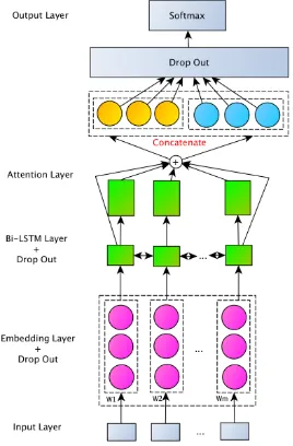
Figure 1: The architecture of our LSTM models. (a) The NN model submitted to Task A, which only incorporates a drop out layer after bi-lstm layer. (b) The NN model explored after contest, which adds attention layer and incorporates additional drop out at both embedding and lstm layers.

2.2.2 Deep Learning

Next, we explored neural networks in subtask A. We modeled all the tweets data through a Bi-LSTM network. The general architecture of the model was depicted in Figure1.

• Input and Embedding Layer: Each tweet was preprocessed by normalizing hyper links and mentions tosomeurlandsomeuseras de-scribed in2.1.1and extracting word n-grams in hashtags as described in2.1.4. Then the tweet was converted into a vector and padded to an equal length (or truncated if the tweet is longer than the pre-defined length). The input vector was fed to the embedding layer (i.e. pre-trained glove.twitter.27B vectors), which converted each word into a distributional vec-tor.

• Bi-LSTM Layer: We used bi-directional L-STMs to model the input sequence. In the bidirectional architecture, two layers of hid-den nodes from two LSTMs captured com-positional semantics from both forward and backward directions of the word sequence.

• Attention Layer: We add attention layer to model the weights of input words follow (Raffel and Ellis, 2016), i.e. learning the weights of hidden states at each time stamp,

then computing the sentence representation via a weighted sum.

• Output Layer:The output of Bi-LSTM was passed to a fully connected (FC) layer, which produced a higher order feature set easily separable for 2 classes. Finally, a softmax layer was added on top of the fully connected layer. The network was trained by minimizing the binary cross-entropy error with ADAM (Kingma and Ba, 2015) for parameter optimization.

3 Experiments and Results

3.1 Datasets

The statistics of the datasets provided by SemEval 2018 task 3 are shown in Table1.

Subtask A Label 0(%) Label 1(%) - -train 1,923 (50.2%) 1,911 (49.8%) - -test 473 (60.3%) 311 (39.7%) -

-Subtask B Label 0(%) Label 1(%) Label 2(%) Label 3(%)

train 1,923 (50.2%) 1,390 (36.3%) 316 (8.2%) 205 (5.3%) test 473 (60.3%) 164 (20.9%) 85 (10.8%) 62 (7.9%)

Table 1: Statistics of datasets in train and test data. Label 0 stands fornon-ironic, label 1 in subtask A is ironic, label 1, 2, 3 in subtask B is respectivelypolarity contrast irony,situational ironyandother verbal irony.

3.2 Evaluation Metric

• Forsubtask A, onlyF1-score ofIronicclass

is used.

F =Fpos

• Forsubtask B, macro-averagedF1-score

cal-culated among all four classes is used.

Fmacro= Fpolar cont+Fsenti+₄ Fother+Fnon

3.3 Experiments on training data 3.3.1 Subtask A: Irony Detection

We used a series of features and explored different machine learning algorithms, in combination with neural networks, in subtask A.

Machine Learning

The count of the train data was only 3,834 and no dev datasets were provided. To fully exploit these data, we used 10-fold cross-validation with data shuffling. The major feature selection work was done with LibLinear L2-regularized logistic regression (LibLinear LR).

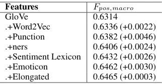
We used the following features in Table2as the baseline features. Since the cross validation oper-ations were done with data shuffling, some fluc-tuations in result might exist. From the table it can be observed that all these features can make contributions to the classifier.

Features Fpos,macro

GloVe 0.6314

.+Word2Vec 0.6336 (+0.0022) .+Punction 0.6382 (+0.0046) .+ners 0.6406 (+0.0024) .+Sentiment Lexicon 0.6432 (+0.0026) .+Emoticon 0.6462 (+0.0030) .+Elongated 0.6465 (+0.0003)

Table 2: Performance of different features on cross-validation shuffling data test. “.+” means to add current features to the previous feature set. The numbers in the parentheses are the performance increments compared with the previous results.

Then we added three other features: Word N-grams, Hashtags and Hashtag unigrams. Each feature had two versions, with or without

Relevant frequency (RF). Simultaneously, we set different word frequency when building lexicon for these features, from frequency threshold 1 to 5. In order to choose features which can improve the performance best, we used

Hill Climbingmethod.

Hill Climbingis a method which can automati-cally extract the best features from a set of given features. Its principle is as follows:

1. Given a Candidate Feature set, traverse each feature and move the feature producing the best performance intoBest Featureset. 2. Traverse the remaining features in

Candidate Featureset, ensemble each one withBest Featureset to train the model. If one feature can lead to better performance than before, move it toBest Featureset. 3. Repeat step 3 until thatCandidate Feature

set is empty.

4. The best feature combination can be obtained by traversingBest Featureset according to the insertion order of each feature.

After runningHill Climbing5 times and extract-ed the features from each first line, we selectextract-ed 7 features, as shown in Table3.

Feature Threshold WithRF

Trigram 4 Yes

Bigram 2 Yes

Hashtag 2 Yes

Hashtag 1 Yes

Hashtag unigram 1 No

Trigram 2 Yes

Unigram 2 Yes

Table 3: The results of hill climbing.

Algorithms Fpos,macro SkLearn Na¨ıveBayes 0.7111 Sklearn LR 0.6953 LibLinear LR 0.6947

Table 4: Performance of three best learning algorithms.

Then we explored the performance of different learning algorithms. Table4 lists the comparison of best three supervised learning algorithms with all above features.

Finally, we made ensemble of three algorithms in Table4. The ensemble score was 0.6982.

Neural Networks

In our LSTM framework, the dimension of word vector was set to 100 and the hidden layers for both LSTM and FC layers were set to 256. The drop out rate was set to 0.2 for preventing overfitting. 10% of the training data were randomly selected as validation set. The best model during training was used in test evaluation stage. We implement the framework based on

seed precision recall f1-score

6815 seed3 0.683908 0.639785 0.661111 6867 seed7 0.705036 0.553672 0.620253 6684 seed11 0.658654 0.709845 0.683292 6789 seed13 0.668142 0.758794 0.710588 6658 seed23 0.692308 0.574468 0.627907 Table 5: Performance of partial neural networks on subtask A on train and dev datasets.

The performance results on train datasets are listed in Table5, and the average is about 0.66.

Ensemble of Machine Learning and Neural Networks

The average performance of machine learning and neural networks were respectively 0.69 and 0.66. We ensembled different results of neural network and of machine learning. Here we used 4 algorithms, i.e., Scikit-Learn’s Na¨ıveBayes, LR,

SVM and LibLinear’s LR, to avoid that label 0 and label 1 were voted same times.

During the ensemble, we also tried another s-trategy. Since we wanted to higher the recall value of positive labels, we ensembled only the data pre-dicted as “label 0” by neural networks. For those “label 1” data, we remained their original labels. The results of this strategy will be discussed in3.4.

3.3.2 Subtask B: Irony Classification

When handling subtask B, we used only machine learning.We conducted two steps in subtask B.

In the first step, the averagef1-macroscore is

between 0.42-0.43. Table 6 shows how much each class is graded, thef1-scores of label 2 and

3 are much lower than that of label 0 and 1. This is caused by imbalance in data distribution.

Features f1-score of

Label 0 Label 1 Label 2 of Label 3 Other features 0.712455 0.649360 0.254167 0.066390 .+URL Unigram T1 0.710811 0.421364 0.282700 0.074074 .+URL Unigram T2 0.712627 0.655994 0.280922 0.105691 .+URL Unigram T3 0.703121 0.648396 0.241015 0.067511 .+URL Unigram T4 0.703121 0.650534 0.280922 0.074689 .+URL Unigram T5 0.709412 0.649573 0.278119 0.075630

Table 6: The f1-scores of each label in subtask B. Here label 0 represents forNon-ironic, 1 forPolarity contrast, 2 for Situational irony, 3 for Other verbal irony.

In the second step, to solve the problem of im-balance in data distribution, we enlarged the data size of label 2 and 3. Label 2 was expanded 6 times, and label 3 was expanded to 10 times. Then we ensembled multi-algorithms. Each algorithm would perform 4 binary-classifications

successive-ly. Finally, we used Scikit-Learn LR for label 0, 1, 2, and Scikit-Learn SVM for label 3. Results are listed in Table7.

Label precision recall f1-score

0 0.669960 0.705148 0.687104 1 0.656558 0.623022 0.639350 2 0.343333 0.325949 0.334416 3 0.167539 0.156098 0.161616

Average score

- 0.459348 0.452554 0.455622 Table 7: The performances of using 4 binary classifications

However, when generating test files, the output results fluctuated remarkably. At last, we didn’t hand in the output result generated by step 2.

3.4 Results on Test Data

Subtask System f1-score (%)

Subtask A

ECNU 0.5931 (20)

THU NGN 0.7054 (1) NTUA-SLP 0.6719 (2) WLV 0.6500 (3)

Subtask B

ECNU 0.2326 (30)

UCDCC 0.5074 (1) NTUA-SLP 0.4959 (2) THU NGN 0.4947 (3)

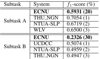
Table 8: Performance of our systems and top-ranked teams on both two subtasks. The numbers in the parentheses are the official rankings. The evaluation metrics in mentioned in3.2.

Table8shows the results of our system and the top-ranked systems provided by the official. Com-pared with the top ranked systems, there’s so much room for improvement in our work. There are sev-eral possible reasons for this.

• First,the overfitting problems is very

seri-ous. The scores during Training and dev pe-riod and test pepe-riod differed significantly. It will be discussed in3.5.

• Second, possibly the features failed to

ex-tract useful information from the test da-taUnlike Word N-Grams, some features, like hashtag, the probability of the same hashtag or matching words appearing in both test files and training files is quite low.

3.5 Supplement results beside the contest 3.5.1 Ensemble of Machine Learning and

Neural Networks on subtask A

Model seedx precision recall f1-score (%)

NN 6815 sd3 0.580282 0.662379 0.618619 (12)

NN 6867 sd7 0.626415 0.533762 0.576389 (27)

NN 6684 sd11 0.532895 0.781350 0.633638 (6)

NN 6789 sd13 0.529279 0.755627 0.622517 (10)

NN+additional dropout 6867 sd7 0.587393 0.65916 0.621212 (11) NN+additional dropout 6684 sd11 0.525000 0.810289 0.637168 (6) NN+additional dropout 6789 sd13 0.537079 0.768489 0.632275 (6) NN+additional dropout+attention 6815 sd3 0.537383 0.739550 0.622463 (10) NN+additional dropout+attention 6867 sd7 0.529870 0.655949 0.5862070 (24) NN+additional dropout+attention 6684 sd11 0.544118 0.7138264 0.617524 (13) NN+additional dropout+attention 6789 sd13 0.574850 0.6173633 0.595349 (19)

Table 9: Performance of pure neural networks on subtask A on test datasets. The number in parentheses is the position of this result if submitted. Performances in Group ‘NN’ are based on Figure 1(a); Performances in Group ‘NN+more dropout’ are based on Figure1(a)with additional drop out settings; and Performances in Group ‘NN+more dropout+attention’ are based on Figure1(b).

Ensemble precision recall f1-score (%)

TOP3 0.400000 0.553055 0.464238 (37)

4+NN, en0 0.450777 0.839228 0.586517 (24)

4+NN, en0 0.452340 0.839228 0.587838 (23)

4+NN 0.404651 0.559486 0.469636 (35)

4+NN, en0 0.493590 0.742765 0.593068 (20)

Table 10: Performance of ensemble on machine learning and neural networks on subtask A and test datasets. The numbers in parentheses represent positions in the official ranking if the result is submitted. The last record is the same asECNU’s.

In Table 10, TOP3 means the ensemble of 3 best algorithms on train datasets. The 4+NN

means using 4 best machine learning algorithms and ensemble them with the results of neural networks. en0 means using the other strategy mentioned in 3.3.1. Hence, the ensemble data using the other strategy enjoys a particular high recall value. Nevertheless, the performance of these results differ greatly that on train datasets.

seed precision recall f1-score (%)

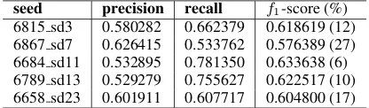
6815 sd3 0.580282 0.662379 0.618619 (12) 6867 sd7 0.626415 0.533762 0.576389 (27) 6684 sd11 0.532895 0.781350 0.633638 (6) 6789 sd13 0.529279 0.755627 0.622517 (10) 6658 sd23 0.601911 0.607717 0.604800 (17) Table 11: Performance of pure neural networks. The numbers in parentheses represent positions in the official ranking if the result is submitted.

In Table 11, the average of f1-scores on pure

neural networks’ results is about 0.61. This phe-nomenon indicates that in our work the training of supervised machine learning appeared to have been overfitted.

3.5.2 Neural Networks on subtask A

In Table9the average of f1-scores on pure neural networks’ results are 0.61, 0.62 and 0.60 for three Groups respectively.

This phenomenon indicates that in our work, the training of supervised machine learning appeared to be overfitted. Moreover, turn on drop out set-tings in more neural network layers can further re-duce overfitting.

However, our attempt of further incorporating attention layer brought negative affect on subtask A’s performance. This may suggest the weighted sum of hidden states probably is not a good repre-sentation of the sentence for irony detection.

4 Conclusion

In this paper, we explored supervised machine learning algorithms and neural networks, detected whether a given tweet was ironic or not, and classified them into four more detailed categories. The result was that the machine learning classifiers overfitted, and neural networks performed better than the traditional training methods. The system performance for subtask A ranked above average, and subtask B didn’t perform so well. In future work, we consider focusing more on exploring the neural networks.

Acknowledgements

References

Mart´ın Abadi, Paul Barham, Jianmin Chen, Zhifeng Chen, Andy Davis, Jeffrey Dean, Matthieu Devin, Sanjay Ghemawat, Geoffrey Irving, Michael Isard, et al. 2016. Tensorflow: A system for large-scale machine learning. InOSDI, volume 16, pages 265– 283.

Steven Bird, Ewan Klein, and Edward Loper. 2009. Natural language processing with Python: analyz-ing text with the natural language toolkit. ” O’Reilly Media, Inc.”.

Rong-En Fan, Kai-Wei Chang, Cho-Jui Hsieh, Xiang-Rui Wang, and Chih-Jen Lin. 2008. Liblinear: A library for large linear classification. Journal of machine learning research, 9(Aug):1871–1874.

Cynthia Van Hee, Els Lefever, and Vronique Hoste. Semeval-2018 task 3: Irony detection in english tweets. In Proceedings of the 12th International Workshop on Semantic Evaluation (SemEval-2018).

Diederik P Kingma and Jimmy Lei Ba. 2015. Adam: A method for stochastic optimization. international conference on learning representations.

Man Lan, Chew Lim Tan, Jian Su, and Yue Lu. 2009. Supervised and traditional term weighting methods for automatic text categorization. IEEE transactions on pattern analysis and machine intelligence, 31(4):721–735.

Man Lan, Guoshun Wu, Chunyun Xiao, Yuanbin Wu, and Ju Wu. 2016. Building mutually beneficial relationships between question retrieval and answer ranking to improve performance of community question answering. pages 832–839.

Christopher Manning, Mihai Surdeanu, John Bauer, Jenny Finkel, Steven Bethard, and David McClosky. 2014. The stanford corenlp natural language processing toolkit. In Proceedings of 52nd annual meeting of the association for computational linguistics: system demonstrations, pages 55–60.

Tomas Mikolov, Ilya Sutskever, Kai Chen, Gregory S Corrado, and Jeffrey Dean. 2013. Distributed representations of words and phrases and their compositionality. neural information processing systems, pages 3111–3119.

Fabian Pedregosa, Ga¨el Varoquaux, Alexandre Gram-fort, Vincent Michel, Bertrand Thirion, Olivier Grisel, Mathieu Blondel, Peter Prettenhofer, Ron Weiss, Vincent Dubourg, et al. 2011. Scikit-learn: Machine learning in python. Journal of machine learning research, 12(Oct):2825–2830.

Jeffrey Pennington, Richard Socher, and Christopher D Manning. 2014. Glove: Global vectors for word representation. pages 1532–1543.

Colin Raffel and Daniel PW Ellis. 2016. Feed-forward networks with attention can solve some long-term

memory problems. Inthe workshop proceedings of ICLR 2016.