Adaptive medial axis approximation for sphere tree construction

Sphere-Tree Construction

Gareth Bradshaw and Carol O’Sullivan

Image Synthesis Group, Dept. of Computer Science, Trinity College, Dublin, IRELAND

Hierarchical object representations play an important role in performing efficient collision han-dling. Many different geometric primitives have been used to construct these representations, which allow areas of interaction to be localized quickly. For time-critical algorithms, there are distinct advantages to using hierarchies of spheres, known as sphere-trees, for object representa-tion. This paper presents a novel algorithm for the construction of sphere-trees. The algorithm presented approximates objects, both convex and non-convex, with a higher degree of fit than ex-isting algorithms. In the lower levels of the representations, there is almost an order of magnitude decrease in the number of spheres required to represent the objects to a given accuracy.

Categories and Subject Descriptors: I.3.5 [Computer Graphics]: Computational Geometry and Object Modeling -Object Hierarchies; I.3.7 [Computer Graphics]: Three-Dimensional Graphics and Realism -Animation

General Terms: Algorithms

Additional Key Words and Phrases: Animation, Collision Handling, Object Approximation, Me-dial Axis Approximation, Simulation Level-of-Detail

1. INTRODUCTION

Collision handling is a major bottleneck in any interactive simulation. Ensuring that objects interact in the correct manner is very computationally intensive and much research has addressed the issues involved with trying to reduce the computa-tional requirements. Researchers often utilize hybrid collision detection algorithms to tackle the problem in various phases. The initial phase of such an algorithm, thebroad phase,aims to efficiently cull out pairs of objects that cannot possibly be interacting. A number of different techniques have been used to achieve this coarse grain detection. These include Sweep & Prune [Cohen et al. 1995; Ponamgi et al. 1997],global bounding volume tables [Palmer and Grimsdale 1995] and overlap tables [Wilson et al. 1998].

Having determined which objects are potentially interacting,the hybrid algo-rithm uses a finer grained algoalgo-rithm to narrow in on the regions of the objects that are in contact. This narrow phase processing typically traverses hierarchical

Authors’ E-Mail : Gareth [email protected]& [email protected]

Permission to make digital/hard copy of all or part of this material without fee for personal or classroom use provided that the copies are not made or distributed for profit or commercial advantage, the ACM copyright/server notice, the title of the publication, and its date appear, and notice is given that copying is by permission of the ACM, Inc. To copy otherwise, to republish, to post on servers, or to redistribute to lists requires prior specific permission and/or a fee.

c

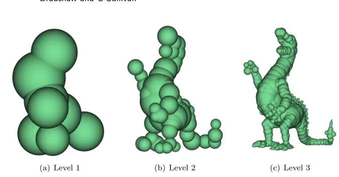
(a) Level 1 (b) Level 2 (c) Level 3

Fig. 1. Example of a dragon approximated with 3 levels of spheres.

representations of the objects,such as that shown in Figure 1,to hone in on the regions of interest. This reduces the amount of work that is required to perform the “exact” collision detection using such algorithms as those described by Palmer and Grimsdale [1995] and Moore and Wilhelms [1988].

Many different geometric primitives have been used for constructing the “Bound-ing Volume Hierarchies” (BVH) used to perform narrow phase processing. These include: Spheres [Quinlan 1994; Palmer and Grimsdale 1995; Hubbard 1995a; 1995b; 1995c; 1996a; O’Sullivan and Dingliana 1999],Axis Aligned Bounding Boxes (AABBs) [van den Bergen 1997],Oriented Bounding Boxes (OBBs) [Gottschalk et al. 1996; Krishnan et al. 1998],Discrete Oriented Polytopes (k-DOPs) [Klosowski et al. 1998],Quantized Orientation Slabs with Primary Orientations (QuOSPOs) [He 1999],Spherical Shells [Krishnan et al. 1998] and Sphere Swept Volumes (SSVs) [Larsen et al. 1999].

There is often a trade-off between the complexity of the bounding volume prim-itives and the tightness of fit that they can achieve. Simpler primprim-itives,such as spheres and AABBs,are quite inexpensive to test for intersections. However,as they provide relatively poor approximations,large numbers are often required to approximate the objects effectively. More complex bounding volume primitives re-quire more expensive intersection tests but,as they often provide tighter approxi-mations,fewer primitives (and hence intersection tests) are required. The following equation has been used by Gottschalk et al. [1996],van den Bergen [1997] and Klosowski et al. [1998] to evaluate various types of bounding volume hierarchies:

where :

T is the total cost of collision detection between two objects,

Nu is the number of primitives updated during the traversal,

Cu is the cost of updating a primitive’s position/orientation,

Nv is the number of overlap tests that are performed,

Cv is the cost of an overlap test between a pair of primitives.

Simple primitives,such as spheres,exhibit low values forCu andCv. As spheres are rotationally invariant,a node can be updated simply by translating its center point to reflect the change in the object’s position and orientation. Testing spheres for overlap is also computationally inexpensive,requiring only a simple distance test. However,as these primitives often do not fit objects well,Nv (and henceNu) can be quite large. More complex primitives,such as OBBs and SSVs,represent the objects more closely and henceNvandNu are lower,but the overlap tests and update costs are generally higher. The table1 below compares spheres and OBBs (using theSeparating Axis Test [Gottschalk et al. 1996]) with respect to Equation 1:

Primitive C_u C_v

Sphere 21=1*t 10

OBB 75=3*r + 1*t 80-200

Although spheres often do not provide particularly tight bounding volumes,there are a number of distinct advantages to their use. Not only are they computationally inexpensive to use at run-time,but each level of the sphere-tree can be used to generate an approximate response [O’Sullivan and Dingliana 1999; Dingliana and O’Sullivan 2000].

This is particularly advantageous when using the interruptible collision detection algorithm. This algorithm,introduced by Hubbard,uses a time-critical traversal of the sphere-trees that is terminated when the allotted time-slice has expired,allowing consistent frame-rate to be maintained [Hubbard 1995a; 1995b; 1995c; 1996a]. As the collisions may never be resolved down to the surface of the objects,the spheres are used to approximate the collisions.

This paper presents a novel sphere-tree construction algorithm,based on Hub-bard’s original medial axis method. The algorithm maintains a medial axis ap-proximation that can be refined as the sphere-tree construction progresses. This ensures that there will always be enough information for the construction of a tight fitting approximation. The rest of the paper is organized as follows: Section 2 discusses the requirements of a good bounding volume hierarchy and gives a brief overview of some of the existing algorithms for the construction of sphere-trees. Section 3 overviews the process of sphere-tree construction within our frame-work and discusses how object sub-division is managed. Section 4 presents the adaptive medial axis approximation algorithm,which extends the existing algorithm to al-low the approximation to be updated as required. Section 5 presents a number of

1_{In this table,ris the cost of rotating a point/vector in 3D andtis the cost of applying a 3D}

new algorithms for the generation of sphere sets from the medial axis approxima-tion. Section 6 evaluates the new algorithms for the approximation of objects,the construction of sphere-trees and their use within interactive simulations. Section 7 presents information about how we construct our sphere-trees for use in real-time interactive simulations. Finally,Section 8 presents conclusions and mentions some future work.

2. EXISTING ALGORITHMS

A number of algorithms have been used for the construction of sphere-trees. Any algorithm that constructs bounding volume hierarchies for collision detection must meet three basic requirements [Hubbard 1995b]:

—the hierarchy conservatively approximates the volume of the object,each level representing a tighter fit than its parent;

—for any node in the hierarchy,its children should cover the parts of the object covered by the parent node;

—the hierarchy should be created in a predictable automatic manner,not requiring user interaction;

—the bounding volumes within the hierarchy should fit the original model as tightly as possible,representing the original model to a high degree of accuracy.

For interactive simulations the emphasis is on achieving high and consistent frame-rates. Therefore,a major concern is how well the hierarchy facilitates this goal. In an interruptible collision handling system the narrow phase algorithm may not fully resolve the collisions. Thus,the approximate collision information,avail-able from the BVH,needs to approximate the points and types of contact (contact modelling) and the resulting response at every level of the approximation [Dingliana and O’Sullivan 2000].

The simplest algorithm for construction of sphere-trees uses the Octree data-structure. The octree is constructed by using recursive sub-division of the object’s bounding cube into 8 smaller cubes. The cubes that cover part of the object are then further sub-divided,continuing down to the required depth. At each level,the nodes of the octree become smaller and hence form successively tighter approximations of the object. The sphere-tree is then constructed by placing a sphere around each of the nodes of the octree. This method has been adopted by Palmer and Grimsdale [1995],Hubbard [1995b] and O’Sullivan and Dingliana [1999]. The simplicity of the algorithm allows it to be quickly and easily implemented and for the sphere-trees to be updated when objects deform. However,as the algorithm does not explicitly use the object’s geometry,the sphere-trees produced often fit the object quite poorly.

Along with the octree method,Hubbard also explored two other methods for the construction of sphere-trees. The first used simulated annealing to improve the fit of the spheres constructed with the octree method. This produced mixed results and so a new algorithm,which makes use of the object’s medial axis,was developed. This algorithm makes explicit use of the object’s geometry,in the form of its medial axis,and produces much tighter fitting sphere-trees than the octree method. However,there are a number of difficulties associated with the construction of the medial-axis approximation and the resulting sphere-tree. This paper presents an algorithm that addresses these problems by using an adaptive medial axis approximation that ensures a tight fitting sphere-tree.

3. HIGH-LEVEL CONSTRUCTION ALGORITHM

This section gives an overview of the new sphere-tree construction algorithm. The algorithm consists of a number of layers. The top layer decomposes the construction into a number of sub-problems by sub-dividing the object into regions. These regions are then approximated with a set of spheres,which are used to further divide the object and hence construct the sub-trees.

The root node of the sphere-tree is the smallest sphere that will enclose the object. This is found using White’s minimum volume enclosing ball routine [White www],which implements the algorithm described by Weltz [1991]. The first level of spheres,the children of the root sphere,are constructed by calling a sphere generation algorithm to approximate the object with at mostNc spheres2.

These spheres are then used to segment the object into a number of regions. Each region defines the areas of the object that must be covered by a set of children spheres. These spheres form the next level of the hierarchy - as children of the sphere that defined the region.

This generic high-level algorithm,outlined as Algorithm 1,forms the basis for all the sphere-tree construction algorithms we use. The generic nature of the top-level algorithm allows different sphere generation algorithms to be implemented and slotted into place. While a number of different sphere generation algorithms have been explored,only the medial axis based algorithms will be discussed in this paper. Prior to this we will detail how the sphere-tree construction algorithm segments the object into regions for approximation.

3.1 Object Segmentation

For each node in the sphere-tree,sphere generation algorithms are used to construct a set of children spheres. In order to ensure that the entire object is approximated, the children must cover the region covered by their parent. Hubbard achieved this by segmenting the medial axis based on how the parent sphere was constructed. To allow for a more generic algorithm,we choose not to use any knowledge of how the sphere was constructed. This makes it much easier to use different types of algorithms from within the top level algorithm and allows the spheres to be post-processed prior to their inclusion in the sphere-tree,e.g. to allow further optimization algorithms to be employed.

2_N

Algorithm 1Sphere-tree construction

Construct set of sample points to cover object’s surface.

Construct initial Voronoi diagram to contain initialNumber

spheres (adaptive algorithm).

Construct bounding sphere object to represent root of

sphere-tree.

FOR each level of the sphere-tree

FOR each sphere in the level (parent sphere)

Determine object region covered by the parent sphere.

Update the Voronoi diagram to cover the parent’s region

with at least minSpheresPerNode spheres (adaptive

algorithm).

Generate reduced set of spheres from the Voronoi

diagram so that the parent’s region is approximated with treeBranchFactor spheres (sphere reducer).

Perform post-processing as desired e.g. run an optimizer

further reduce the error.

Add reduced set of spheres to sphere-tree as children of

the parent sphere.

Therefore,we need to be able to determine the regions of the object covered by each sphere in an arbitrary set of spheres. If we were to cover every region contained within the each sphere,we would introduce a lot of duplication into the hierarchy by approximating the overlapping regions multiple times. This would be very wasteful as the same area would be covered many times,further contributing to the overlap.

A more desirable situation is to divide the object into sub-regions with as little overlap as possible. This is achieved by dividing any overlapping regions between the spheres. In a region covered by a number of spheres,each part of the object need only be covered by one set of children spheres. While it is advantageous to have the interior of the object filled with spheres,to prevent tunnelling,we require that only the surface of the object be completely covered. Some algorithms,particularly those based on the medial axis,usually fill the interior of the object quite well anyway.

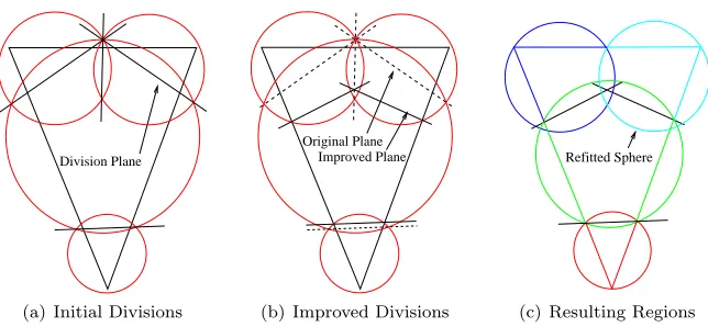
The surface of the object is represented by an arbitrarily large set of sample points. To segment the object into regions we simply choose the sub-set of points that represents the surface within that area. Any points that lie in the overlap between two spheres can be covered by either of the sets of children. To determine which points are to be covered by each set,a dividing plane is constructed through the intersection. Points are distributed based on which side of the plane they lie on.

Division Plane

(a) Initial Divisions

Improved Plane Original Plane

(b) Improved Divisions

Refitted Sphere

(c) Resulting Regions

Fig. 2. Dividing the object into distinct regions using dividing planes.

arbitrary configuration,the spheres tend to be of varying sizes. In this case the region associated with the large central sphere is much bigger than the regions associated with the other spheres. Thus,the children of this sphere will potentially have a looser fit than the other child sets. It is very desirable that the regions divide the object as evenly as possible without affecting the fit of the spheres. A simplex based optimization algorithm is used to move the dividing plane between each pair of spheres so as to make the division as even as possible,as shown in Figure 2(b).

Once we have established the regions to be covered by each of the spheres,re-placement spheres can be created. These new spheres are only required to cover parts of the surface that are not covered by any other spheres,which allows tighter fitting spheres to be created,as shown in Figure 2(c).

4. ADAPTIVE MEDIAL AXIS CONSTRUCTION

The medial axis of an object represents itsskeleton and can be defined as the cen-ters of a set of maximally sized spheres that fill a figure [Blum and Nagel 1978]. Constructing the medial axis for a polyhedral model is a complicated and com-putationally expensive task. For the purposes of constructing sphere-trees,an ap-proximate medial axis suffices. Hubbard used a static medial axis approximation for the construction of sphere-trees. We have extended this to allow the medial axis approximation to be updated during the sphere-tree construction. Like Hub-bard,we use a Voronoi diagram to represent the medial axis. This section gives an overview of how the Voronoi diagram is used to approximate the object. For full construction details see [Hubbard 1995b; 1996b].

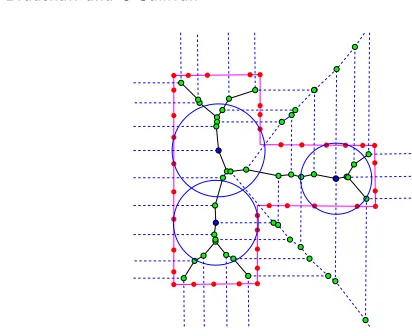
A Voronoi diagram is constructed from a set of forming points. Each cell within the Voronoi diagram represents the region of space that is closer to its forming point than any of the other forming points. When the set of points is distributed over the surface of the object,a sub-set of the faces,which lie between the cells, forms an approximation of the medial axis.

Fig. 3. Spheres are placed on the Voronoi vertices that are inside the object.

around them,approximate the object’s shape. Figure 3 shows an example of this in 2D,where circles are placed around the internal vertices and touch the surface in (at least) 3 places.

There are a number of difficulties associated with the construction of a medial-axis approximation for generating sphere-trees. The problems arise when choosing the set of points from which to make the Voronoi diagram. It is extremely difficult to find a set of points that results in a set of spheres that will completely cover the object. This results in an approximation that contains holes which will allow objects to interpenetrate. It is also impossible to determine a priori how to construct a medial axis approximation that will lead to a tight fitting sphere-tree. We favor an adaptive medial axis construction algorithm,which addresses these problems.

This algorithm ensures that the medial spheres,and hence the sphere-tree will always cover the entire object. It also allows the medial approximation to be up-dated so that there is always a sufficient number of spheres from which to construct the sphere-tree,and that the spheres fit the object to a high degree of accuracy.

The adaptive medial approximation algorithm is iterative in nature. It starts with an existing medial axis approximation or a single sphere that encloses the object. The first part of the algorithm is to ensure that the set of medial spheres covers the object’s surface. The set of medial spheres,the spheres around the internal vertices,is not guaranteed to cover the entire surface and so extra spheres are placed around external vertices to complete the coverage. The second phase of the adaptive algorithm is to improve the current approximation by adding more sample points. The position of each new sample point is chosen so that the worst sphere in the current approximation will be replaced with tighter fitting ones.

4.1 Completing Coverage

and less frequent.

Using this representation makes it simple to ensure that the model is completely covered. Points that are not covered can be dealt with by adding additional spheres to the medial set. Each Voronoi cell has a number of vertices,which between them represent a set of spheres that cover the entire cell. Thus,to cover a point,only the vertices that make up the cell containing the point need to be considered.

There are several criteria that could be used to choose the sphere to cover each point. The smallest sphere,or the sphere with the lowest error,would help to produce a tight fitting approximation,whereas choosing the largest sphere would potentially cover a number of other uncovered points,requiring less of the spheres in the approximation to be “coverage spheres”. As the adaptive algorithm is able to replace poor fitting spheres,these spheres will subsequently be replaced if they affect the quality of the approximation.

4.2 Iterative Improvement

The second phase of the adaptive medial axis approximation algorithm is the itera-tive improvement step. During each iteration of the algorithm,having marked the medial (and coverage) spheres,the sphere with the worst fit is replaced3.

To replace the chosen sphere,a new point is inserted into the Voronoi diagram. Recall,the vertex will be used to construct a sphere whose radius is equal to the distance from the vertex to its forming points. If the center of the sphere is inside the object,an upper bound on how far this sphere hangs outside the surface of the object is given by:

e=r− q−v (2)

where:

e is the distance the sphere protrudes past the surface, r is the radius of the sphere,

v is the vertex being used to make the sphere, q is the surface point closest to v.

Inserting a new sample point atqresults in a new cell being added to the Voronoi diagram. The spheres created around the vertices of this cell will pass through q and so reduce the error to 0 at that point,as seen in Figure 4(b).

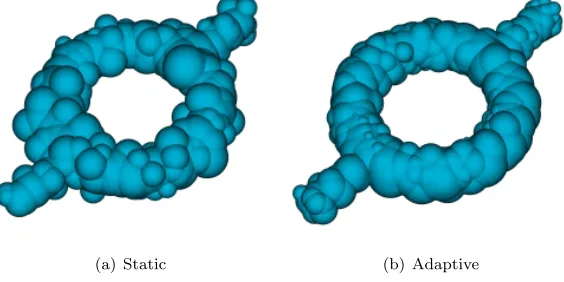
Figure 5 shows a comparison between the adaptive and static algorithms. The adaptive algorithm clearly produces a closer approximation of the object,with the static algorithm producing a very uneven and bumpy result.

5. SPHERE GENERATION

The top level sphere-tree construction algorithm,detailed in Section 3,divides the object into regions which must be approximated with a specified number of spheres. We have explored a number of generation algorithms [Bradshaw 2002],a sub-set of which will be discussed in this section.

3_{As each sphere is associated with a Voronoi vertex, the vertices of the Voronoi diagram have a}

e

v _r q

(a) Before (b) After

Fig. 4. Addition of a new point to reduce the error of the approximation.

(a) Static (b) Adaptive

Fig. 5. Comparison between static and adaptive sampling (1,000 spheres).

The sphere generation algorithms maintain a Voronoi diagram that approximates the medial axis of the object. When the sphere generator is asked to approximate a region of the object,this Voronoi diagram is updated,using the adaptive algorithm discussed in Section 4,so that the set of medial spheres is of sufficient quality to allow a tight approximation. Typically we specify that the set of spheres contains 10 times the target number of spheres and that the worst sphere in the set has an error that is a fraction (typically 1₂ or 1₄) of the parent sphere’s error. Having updated the medial axis approximation,the sphere generation algorithms construct the group of spheres for the sphere-tree.

5.1 Merge

The “Merge” sphere reduction algorithm,loosely based on Hubbard’s algorithm, reduces the sub-set of medial spheres by successively combining pairs of spheres. Each sphere is allowed to merge with a number of other spheres,its neighbors. Initially,each sphere is given a set of neighbors that correspond to the vertex’s neighbors within the Voronoi diagram.

of spheres is merged,a new sphere,covering the union of these two sets,is con-structed. Hubbard used Ritter’s approximate bounding sphere algorithm for the construction of this sphere [Ritter 1990]. We favor a more accurate method,which constructs three spheres and uses the one with the tightest fit. Two of the spheres are constructed by growing the existing spheres to cover the combined set of points. The third sphere is constructed using White’s minimum volume enclosing ball al-gorithm [White www]. This scheme allows the sphere to remain close to the medial axis unless it is beneficial to move it,which allows for a tighter approximation.

As the merging of a pair of spheres produces a new sphere,the set of merges must be updated. The neighbors of each of the merged spheres will become neighbors of each other,resulting in new potential merges. In order to ensure that we are always able to reduce the sphere set,any spheres that end up with no neighboring spheres are given a new set of neighbors,containing any of the remaining spheres it intersects. In the event that this results in an empty set of neighbors,the sphere is made a neighbor of all the remaining spheres in the set. The reason for limiting the pairs of spheres that may be combined is to reduce the computational cost of the reduction process. As the number of pairs isO(n2) it would be very expensive to consider every pair. However,when the number of spheres becomes sufficiently low,it becomes feasible to consider every pair for merging. This is typically done when we reach 2 or 3 times the target number of spheres.

At each iteration of the merge algorithm,a pair of spheres is combined to reduce the number of spheres by one,using a greedy algorithm. At each iteration,the merge that results in the lowest error is used. We give special consideration to merges that actually reduce the error in the approximation and we refer to these as “beneficial merges”. As an approximation is only as good as its worst error,we favor merges that improve the worst spheres in the approximation. We do not treat other beneficial merges as a special case as we have found that this can adversely affect the final results.

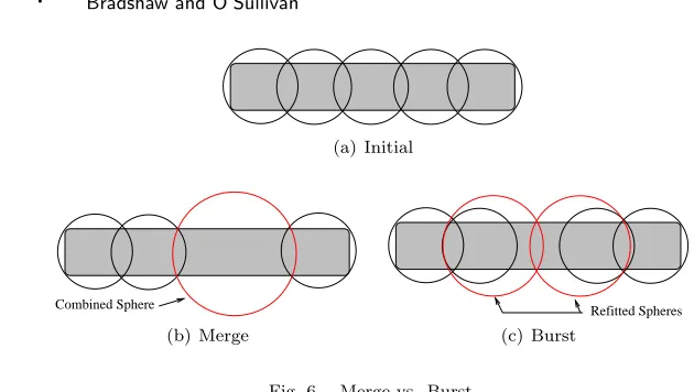
5.2 Burst

One of the limitations of the merge algorithm is that when a pair of spheres is merged,the increase in error is localized to the new sphere rather than being dis-tributed across the object. Take for example,the arrangement shown in Figure 6(a). When the set is reduced a new sphere is created to cover the area previously covered by two spheres. This results in a sphere with a much larger error than the rest,as shown in 6(b).

The “Burst” algorithm aims to address this problem by allowing more of the spheres to absorb the increase in error. Removing (or bursting) one of the spheres and using the surrounding spheres to fill in the gap will better distribute the error introduced by decreasing the number of spheres. Figure 6(c) shows the result of removing one of the spheres from the set. In this scenario the worst error in the approximation has been reduced.

(a) Initial

Combined Sphere

(b) Merge

Refitted Spheres

(c) Burst

Fig. 6. Merge vs. Burst.

the remaining spheres,each point will be assigned to the sphere that is closest to covering it. Finding this sphere involves measuring the distance from the point to the shell of the spheres as follows:

D(S, P) =Sc−P −Sr (3) where:

D(S, P) is the distance from sphereS to pointP,

Sc is the center of sphereS,

Sr is the radius of sphereS.

The value of D(S, P) will become negative if the point P is already contained within the sphereS,which will indicate that the point should definitely be assigned to that sphere. Finally,each sphere that is assigned new points must be updated so that it covers the new set of points.

This algorithm operates in a similar fashion to the merge algorithm,removing the sphere that will introduce the least error at each iteration. Unlike the merge algorithm,the burst algorithm benefits greatly from the use of beneficial bursts. Ordinarily the cost of a burst is defined as the sum of the errors of all the spheres involved. A beneficial burst is defined as a burst that reduces the worst error of the spheres used to fill in the gaps created. Thus,at each iteration of the algorithm, the burst that reduces this error by the largest amount is chosen. If there are no beneficial bursts available,the burst with the lowest cost is chosen.

5.3 Expand & Select

The burst algorithm for sphere reduction was designed to allow the error intro-duced by the removal of a sphere to be distributed amongst some of the remaining spheres. While there are a number of situations where this will improve on the merge algorithm,it allows only the neighboring spheres to absorb the increase in error. A much better strategy would be to select a set of spheres that distribute the error evenly between them.

fit. Equation 2 gave us a metric to measure the distance from a sphere to the surface. This equation can be rearranged to allow us to compute the radius required,for a given sphere,to make it hang over the surface by a given amount,e. Thus for a given value ofe,the radius of a sphere that will hang over the surface by at most

ecan be computed as:

r=e− q−c (4)

where:

r is the radius of the sphere,

e is the distance the sphere protrudes past the surface, c is the center of the sphere,

q is the point on the surface.

To approximate the object,the medial spheres are expanded to the desired stand-off distance (e),using Equation 4,and the spheres that do not uniquely cover any part of the object are discarded. For convex bodies the stand-off distance is exactly equal to the worst distance from the sphere to the surface. For non-convex bodies, the stand-off distance is an over-approximation of this error.

Is it not possible to pre-determine the value forethat will result in the required number of spheres being selected. In order to construct a set containing a certain number of spheres,we must search for the correct value of e. A simple search algorithm,derived from the Binary Search,finds the lowest value ofethat results in a set containing the required number of spheres.

The job of selecting the minimum number of expanded spheres that cover an object is a complicated one. As the set of spheres from which the reduced set is drawn is potentially quite large,it would be very expensive to try every combination of spheres. Instead of looking for this global optimum,we can try to find a good minimal set of spheres,which will be a set from which none of the spheres can be removed without exposing part of the surface.

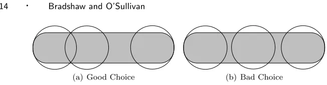
A greedy algorithm allows us to choose the set of spheres without having to eval-uate a large number of combinations. The algorithm maintains the set of currently selected spheres and additional spheres are chosen from the remaining ones until the desired region is completely covered. In order to decide which sphere to choose, each sphere must be ranked according to its potential to keep the set of spheres small. The first obvious choice would be to rank each candidate by the area of previously uncovered surface contained within it. This will allow the algorithm to cover the largest amount of the object at each iteration. As with all greedy algo-rithms,this aims to make the biggest gain at each stage but does not guarantee to find the global optimum.

com-(a) Good Choice (b) Bad Choice

Fig. 7. When selecting a set of spheres to cover the object, the choice of sphere may result in gaps being formed, which will require extra spheres to fill them.

plete the approximation. However,the second option,illustrated in Figure 7(b), will require two more spheres,one on either side of the third sphere.

Another way of approaching this is to rank the spheres by the number of remain-ing spheres that it makes redundant. Rankremain-ing the spheres in this way will tend to select spheres that cover complicated areas of the object first,especially when the set of spheres has been constructed using the adaptive medial axis approximation algorithm. It will also tend to choose spheres that cover areas near previously se-lected spheres as these spheres will help the new sphere to eliminate more of the remaining spheres,increasing its ranking. This will favor the configuration shown in Figure 7(a). These heuristics have been calledMaxCover and MaxElim respec-tively,the latter being used as it produces marginally better results in practice.

6. EVALUATION

This section compares the various algorithms for both object approximation and sphere-tree construction. The algorithms have been compared using a number of simple geometric shapes including a cube,an ellipsoid,a cylinder,a torus,a cone, an “S” shape created from NURBS surfaces and an “L” with square cross sections. A number of complex models have also been used,including a Bunny4, a Cow, a Dragon5,a lamp,a shamrock,a teapot and various letters of the alphabet. To allow a large number of bodies to be used in real-time simulations,the models of the bunny,the cow and the dragon were simplified using Garland’sQSlim software [Garland 1999] to reduce the number of faces that need to be rendered. A selection of the models used can be seen in Figure 8.

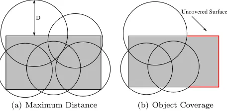
There are a number of factors that must be considered when approximating an object with spheres. As stated in Section 2,the spheres should approximate the object’s surface to a high degree of accuracy and should cover the entire object. The tightness of fit can be measured as the maximum distance from the surface of the spheres to the actual surface of the object,as illustrated in Figure 9(a). This represents an upper bound on the distance between two objects when they are falsely thought to be involved in a collision,which has been found to be one of the most important factors influencing a viewer’s ability to perceive bad collisions [O’Sullivan and Dingliana 2001]. The amount of the object not covered by the approximation can be either the volume of the object that is not contained within the union of the spheres,or the amount of surface area that is not covered by this union. For this evaluation we will choose the latter,illustrated in Figure 9(b),as

4_{Data from http://graphics.stanford.edu/data/3Dscanrep/}

(a) The Bunny (b) The Dragon (c) The Lamp

Fig. 8. Some of the models used for testing the algorithms.

D

(a) Maximum Distance

Uncovered Surface

(b) Object Coverage

Fig. 9. Measuring error and coverage in sphere approximations.

it is not critical to fill the object entirely as long as the surface is well covered. The initial analysis is concerned with the geometric properties of the approxi-mations and sphere-trees that result from the various algorithms. Later analysis considers the use of the resulting sphere-trees in an interruptible collision handling system.

6.1 Medial Axis Construction

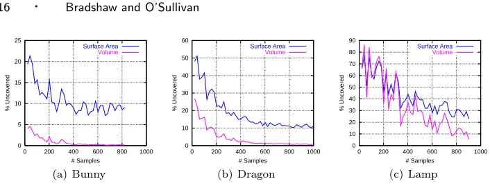
Section 4 detailed the adaptive medial axis construction algorithm,which addresses the problems associated with the previous approaches. The algorithm aims to create a set of spheres that approximate the object closely and does not contain any gaps. Figure 10 shows the amount of the model that is left uncovered by the existing medial axis approximation,both in terms of surface areas and volume. For the more complex models,the static sampling scheme often provided rather poor coverage of the object. As the number of samples increases the coverage generally improves, but a large amount of uncovered surface can remain.

0 5 10 15 20

0 200 400 600 800 1000

% Uncovered

# Samples

Surface Area

Volume

(a) Bunny

0 10 20 30 40 50

0 200 400 600 800 1000

% Uncovered

# Samples

Surface Area

Volume

(b) Dragon

0 10 20 30 40 50 60 70 80

0 200 400 600 800 1000

% Uncovered

# Samples

Surface Area

Volume

(c) Lamp

Fig. 10. Coverage statistics for the sets of medial spheres.

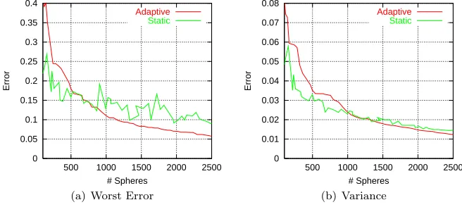
exhibits a lower worst error than using static sampling,although for some models it starts out worse and then improves quite quickly. The adaptive algorithm also often exhibits a decrease in the variance across the approximation,shown in the second graph (b). This is due to the algorithm choosing to improve the worst fitting sphere at each iteration. Thus spheres with large error are replaced while those with lower values are left alone. Although there is not a massive decrease in either error or variance,the adaptive algorithm does maintain coverage of the object whereas the static sampling method can often leave areas of the objects uncovered.

6.2 Sphere Reduction

Having constructed a large set of spheres,which approximate the geometry of the object,the sphere-tree construction algorithm needs to reduce the number of spheres down to the size required for the sphere-tree. Section 5 presented a number of algorithms that aim to improve on Hubbard’s original algorithm.

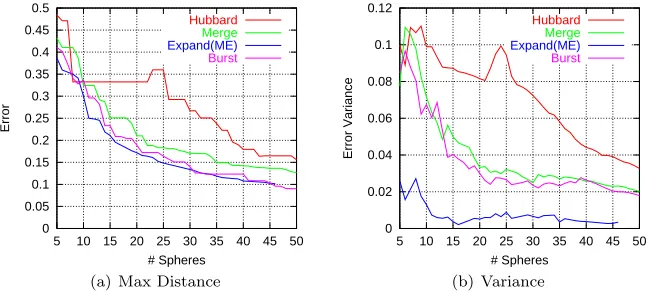
Figures 14 - 16 compare these sphere reduction algorithms. Each algorithm generates the required number of spheres from a set of 500 medial spheres,which were generated using the adaptive sampling algorithm. The first graph (a) compares the algorithms in terms of the distance from the spheres to the surface. The second graph (b) compares the variance of these distances across the approximation.

As expected,the new merge algorithm shows an improvement over Hubbard’s merging strategy. This algorithm certainly reduces both the worst error and vari-ance in the sphere sets. The expand algorithm generates sets of spheres with very low error variance. For convex shapes this variance will be zero,but for non-convex objects some variation is experienced. This is a result of the equation used for computing the sphere’s radius,Equation 4,which over-approximates the error for non-convex bodies. The expand algorithm generally exhibits a lower worst error than either Hubbard’s or the merge algorithm. This is due to the way that the algorithm distributes the error evenly between all the spheres in the resulting set. The burst algorithm further improves the fit of the reduced sets of spheres. Al-though the variance in the set of spheres is higher than the expand algorithm,the worst fit is often better.

0 0.1 0.2 0.3 0.4 0.5 0.6 0.7

500 1000 1500 2000 2500

Error

# Spheres Adaptive

Static

(a) Worst Error

0 0.02 0.04 0.06 0.08 0.1 0.12 0.14 0.16

500 1000 1500 2000 2500

Error

# Spheres Adaptive

Static

(b) Variance

Fig. 11. Static vs. Adaptive sampling for the construction of the medial set of the Bunny.

0 0.05 0.1 0.15 0.2 0.25 0.3 0.35 0.4

500 1000 1500 2000 2500

Error

# Spheres Adaptive

Static

(a) Worst Error

0 0.01 0.02 0.03 0.04 0.05 0.06 0.07 0.08

500 1000 1500 2000 2500

Error

# Spheres Adaptive

Static

(b) Variance

Fig. 12. Static vs. Adaptive sampling for the construction of the medial set of the Dragon.

0 0.05 0.1 0.15 0.2 0.25 0.3

500 1000 1500 2000 2500

Error

# Spheres Adaptive

Static

(a) Worst Error

0 0.01 0.02 0.03 0.04 0.05 0.06 0.07 0.08

500 1000 1500 2000 2500

Error

# Spheres Adaptive

Static

(b) Variance

0 0.1 0.2 0.3 0.4 0.5 0.6 0.7 0.8

5 10 15 20 25 30 35 40 45 50

Error # Spheres Hubbard Merge Expand(ME) Burst

(a) Max Distance

0 0.05 0.1 0.15 0.2 0.25 0.3

5 10 15 20 25 30 35 40 45 50

Error Variance # Spheres Hubbard Merge Expand(ME) Burst (b) Variance

Fig. 14. Comparison of sphere reduction techniques for the Bunny.

0 0.2 0.4 0.6 0.8 1 1.2 1.4

5 10 15 20 25 30 35 40 45 50

Error # Spheres Hubbard Merge Expand(ME) Burst

(a) Max Distance

0 0.05 0.1 0.15 0.2 0.25 0.3 0.35 0.4

5 10 15 20 25 30 35 40 45 50

Error Variance # Spheres Hubbard Merge Expand(ME) Burst (b) Variance

Fig. 15. Comparison of sphere reduction techniques for the Dragon.

0 0.05 0.1 0.15 0.2 0.25 0.3 0.35 0.4 0.45 0.5

5 10 15 20 25 30 35 40 45 50

Error # Spheres Hubbard Merge Expand(ME) Burst

(a) Max Distance

0 0.02 0.04 0.06 0.08 0.1 0.12

5 10 15 20 25 30 35 40 45 50

Error Variance # Spheres Hubbard Merge Expand(ME) Burst (b) Variance

there are no values greater than 25. When trying to fit a set of say 30 spheres,the algorithm can find a set of either 25 or 55 spheres. The algorithm opts for the set of 25 spheres,as it is within the acceptable size,but these cases are omitted from the graphs.

6.3 Sphere-Tree Construction

The top level sphere-tree construction algorithm uses the sphere reduction algo-rithms to generate the sets of spheres that make up the sphere-tree. Figures 17 - 19 compare the sphere-trees generated using various algorithms. All tests were con-ducted with a tree branching factor of 8. This number was used as it provides a reasonable level of sub-division without incurring too much computational costs within the traversal algorithm. All the algorithms used a set of 5000−10000 points to represent each object.

For the bunny,Hubbard’s algorithm used a medial axis approximation containing circa2500 spheres,for both the dragon and lamp this was increased tocirca 20000 as both models contained regions that were hard to cover. For the other algorithms the medial axis initially contained 500 spheres and was dynamically refined so that each region had 1₂ the error of the parent sphere and at least 100 spheres from which 8 were to be produced.

The first graph (a) in each set shows the number of spheres generated for each level of the hierarchy. It is clear from the graphs that the algorithms do not always produce a complete sphere-tree,i.e. a sphere-tree that has the maximum allowable nodes for a given branching factor. The merge/burst algorithms often create sets of spheres that contain contain redundant spheres. These spheres contribute nothing to the approximation as all the areas of the surface that they cover are also covered by other spheres. Thus these spheres are discarded and their descendants are not computed. The expand algorithm often has difficulty choosing a set of spheres that contains the maximum number of spheres and so it chooses the largest set of spheres that contains less than the maximum allowable number of spheres.

0 50 100 150 200 250 300 350 400 450 500 # Spheres Hubbard Merge Burst Expand Combined

(a) # Spheres

0 0.05 0.1 0.15 0.2 0.25 0.3 0.35 0.4 0.45 Error Hubbard Merge Burst Expand Combined

(b) Worst Error

Fig. 17. Comparison of sphere-trees for the Bunny.

0 100 200 300 400 500 600 # Spheres Hubbard Merge Burst Expand Combined

(a) # Spheres

0 0.1 0.2 0.3 0.4 0.5 0.6 Error Hubbard Merge Burst Expand Combined

(b) Worst Error

Fig. 18. Comparison of sphere-trees for the Dragon.

0 100 200 300 400 500 600 # Spheres Hubbard Merge Burst Expand Combined

(a) # Spheres

0 0.05 0.1 0.15 0.2 0.25 0.3 0.35 0.4 0.45 Error Hubbard Merge Burst Expand Combined

(b) Worst Error

Bunny Dragon Lamp

Hubbard 69 1629 1454

Merge 473 595 428

Burst 2083 2000 456

Expand 284 342 1474

Combined 2131 1353 894

Table I. Sphere-tree construction times (in seconds).

algorithm keeps the spheres in their original position,on the approximated medial axis,there are a number of situations where the resulting set of spheres may be fairly poor. For example,when creating a small set of spheres to cover a tube,a good arrangement of spheres would have them centered in the hollow part of the tube. The expand algorithm would center the spheres in the walls of the tube and so result in a very poor approximation. The merge algorithm is a lot more general purpose,and can be used when the expand algorithm fails to produce a good set of spheres.

The times taken to construct the sphere-trees can be seen in Table I6. When Hubbard’s algorithm is used with a small set of medial spheres,the time taken is very small,e.g. for the Bunny. However,for larger sets the algorithm can take 30 minutes to construct the sphere-tree. The overall processing times of our algorithms are comparable to that of Hubbard’s algorithm while providing tighter fitting ap-proximations. The burst algorithm is often the slowest of our new algorithms as it has a lot of house-keeping information to maintain.

6.4 Simulation

To further evaluate the sphere-tree generation algorithms,the behavior of the sphere-trees during simulation was also tested. During these simulations,objects were positioned and oriented randomly about a sphere and were given a random velocity towards its center. The motions of the objects and their response to col-lisions were computed using a commercial dynamics system that uses an “exact” collision detection algorithm and a complex-friction dynamics model.

At each time-step,the colliding pairs were created by testing their bounding spheres. The sphere-trees for these objects were then traversed as they would be in the interruptible collision detection algorithm. The sphere-tree traversals were interrupted at regular intervals and the approximate collisions evaluated. The er-ror associated with each pair of colliding spheres is computed as the sum of the spheres’ errors. As the error associated with a sphere is the largest distance from the surface of the sphere to the surface of the object (Hausdorff distance) this pro-vides an upper-bound for the true separation between the objects. Each of the new algorithms are compared to a reference sphere-tree,i.e. that constructed with Hubbard’s algorithm. For each interruption time,the average improvement is com-puted. This is expressed as the fraction of the reference tree’s error that is present for the new sphere-trees. For example,for each frame (at a given interruption inter-val),the merge sphere-tree is evaluated by computing _ErrorError_{Ref erence}Merge . These values

are then averaged over the frames of 5 simulations,using a new random position (and orientation) for each object for each run.

Figures 20 - 22 present results for simulations containing 20 objects. The hori-zontal axis of each of the graphs shows the interruption interval,expressed in terms of the number of primitive operations performed,i.e. sphere updates and overlap tests. The amount of work done before interruption is computed using Equation 1, where the values of Cu and Cv are 2 and 1 respectively. These values represent the relative number of floating point operations performed in updating a sphere’s position (21 floating point operations) and in testing two spheres for overlap (10 floating point operations). The first graph (a) in each set shows the fraction of the worst error present in the approximations and the second (b) shows the relative number of colliding pairs produced by the different algorithms.

Each of the new sphere-reduction algorithms show a definite reduction in error. For complex models,such as the Bunny,the combined algorithm quickly falls to as little as 50% of the error resulting from the existing algorithm (see Figure 20(a)). For the simpler shapes,this value has been as low as 20%. The algorithms also show significant reductions in the numbers of pairs of colliding spheres that result from the traversal. This represents a reduction in the amount of work that will need to be done by the later stages of the collision handling system,i.e. contact modelling and collision response. For the models shown,the number of resulting collisions has decreased to as little as 20% as the tighter fitting sphere-trees produce less false positives in the collision detection.

6.5 Interruptible vs. Exact Collision Detection

As stated in Section 1,interruptible collision detection algorithms allow us to per-form collision detection in a time-critical fashion. This limits the time that can be spent performing the collision handling so that the desired frame-rate can be maintained.

Normally in an interactive simulation the interruptible algorithm will be given a time-slice that maintains the desired frame rate. The algorithm approximates the collisions as well as it can within the allowed time. The interruptible algo-rithm,implemented as part of our real-time collision handling framework,has been compared to two existing algorithms,namely RAPID[Gottschalk et al. 1996] and SOLID[van den Bergen 1997]. Both these packages provide narrow-phase process-ing based on boundprocess-ing volume hierarchies,RAPID uses OBB-trees whereas SOLID uses AABB-trees.

Figure 23 shows the amount of time each algorithm spent performing collision detection between a large number of bodies. As with the previous graphs,the sim-ulation was controlled by a commercial dynamics package. The simsim-ulation started out with 200 bodies positioned randomly above the open end of a cone. As the simulation progressed the bodies fell,under gravity,and piled up in the bottom of the cone,which caused the number of interactions to grow dramatically.

The graphs show the time taken to perform narrow phase collision detection using RAPID,SOLID and our interruptible algorithm. The time-slice for our interrupt-ible algorithm was limited to 0.1,0.05 and 0.025 seconds,labelled 10fps,20fpsand 40fpsrespectively.

0.3 0.4 0.5 0.6 0.7 0.8 0.9 1 1.1 1.2

0 5000 10000 15000 20000 25000 30000

Fraction of Error

Interruption Interval (# Operationsi)

Merge

Expand

Burst Combined

(a) Worst Error

0.1 0.2 0.3 0.4 0.5 0.6 0.7 0.8 0.9 1 1.1

0 5000 10000 15000 20000 25000 30000

Fraction of Collisions

Interruption Interval (# Operationsi)

Merge

Expand

Burst Combined

(b) Resulting Contacts

Fig. 20. Comparison of sphere-trees at various interruption times for the Bunny (20 objects).

0.3 0.4 0.5 0.6 0.7 0.8 0.9 1

0 5000 10000 15000 20000 25000 30000

Fraction of Error

Interruption Interval (# Operationsi)

Merge

Expand

Burst Combined

(a) Worst Error

0.1 0.2 0.3 0.4 0.5 0.6 0.7 0.8 0.9 1 1.1

0 5000 10000 15000 20000 25000 30000

Fraction of Collisions

Interruption Interval (# Operationsi)

Merge

Expand

Burst Combined

(b) Resulting Contacts

Fig. 21. Comparison of sphere-trees at various interruption times for the Dragon (20 objects).

0.2 0.3 0.4 0.5 0.6 0.7 0.8 0.9 1

0 5000 10000 15000 20000 25000 30000

Fraction of Error

Interruption Interval (# Operationsi)

Merge

Expand

Burst Combined

(a) Worst Error

0.1 0.2 0.3 0.4 0.5 0.6 0.7 0.8 0.9 1

0 5000 10000 15000 20000 25000 30000

Fraction of Collisions

Interruption Interval (# Operationsi)

Merge

Expand

Burst Combined

(b) Resulting Contacts

0 0.05 0.1 0.15 0.2

0 2 4 6 8 10 12 14 16

Time (sec)

Frame Number (x100)

RAPID SOLID 10fps 20fps 40fps (a) Bunny 0 0.05 0.1 0.15 0.2

0 2 4 6 8 10 12 14 16

Time (sec)

Frame Number (x100)

RAPID SOLID 10fps 20fps 40fps (b) Dragon 0 0.05 0.1 0.15 0.2

2 3 4 5 6 7 8 9 10 11

Time (sec)

Frame Number (x100)

RAPID SOLID 10fps 20fps 40fps (c) Lamp

Fig. 23. Algorithm comparisons.

than the allotted time doing the collision detection. As the number of collisions increases the time increases until it reaches the desired maximum. The traditional algorithms are not able to stop during their processing and therefore the time continues to increase. This results in the collision detection taking an increasing amount of time,which will adversely effect the frame-rate of the simulation. For example,from Figure 23(a) it can be seen that RAPID required almost 0.15 seconds to perform collision detection for frame 1000 which means that it would be impos-sible to have a frame rate higher than about 7fps in any simulation that contains such a large number number of interactions between the bodies. Obviously,RAPID and SOLID return the exact points of contact whereas only approximate data will be returned by the interruptible algorithm. However,an approximate response may be computed from this data,thus allowing for graceful degradation of the collision handling [Dingliana and O’Sullivan 2000].

7. SPHERE-TREE CONSTRUCTION FOR REAL-TIME ANIMATION

The sphere-tree construction algorithms presented in this paper can be configured to construct sphere-trees with different attributes. As our aim is to approximate objects for performing collision handling within real-time interactive animations, our goal has been to approximate the object as tightly as possible at each level of the sphere-tree. This optimizes the approximation to allow interruption to occur at any stage of the processing. If the simulations were to contain only a few complex objects,interruption would generally occur quite far down the tree and it may be advantageous to loosen the fit at the top levels if it improved the fit lower down.

It is quite difficult to decide how many branches and levels there should be in the sphere-tree. We have found that for most objects,a branching factor between 6 and 10 is sufficient to sub-divide the object and maintain a tight fit. If the branching factor is too big then the trees are very bushy and produce a lot of work for the traversal algorithms. If,however,the branching factor is too small the object may not be approximated well. For example,it is very difficult to approximate a cube using 5 spheres. Medial based algorithms typically approximate a cube well using a set of 9 spheres with a large one in the center and 8 smaller ones at the corners. For all the examples in this paper we have used a branching factor of 8.

However,if too few are used the approximation might be very poor. The adaptive algorithm tackles this problem by dynamically increasing the number of spheres to keep the approximation tight. Through our experiments we have found that an initial approximation containing 500−1000 spheres is sufficient for generating the top level of spheres,and that using more spheres does not significantly affect the results.

We have explored many different algorithms for constructing the sphere-tree from the medial axis approximation. We have found that using a combination of two different algorithms generally gives the best results. The expand algorithm,detailed in Section 5.3,generally produces very tight fitting approximations. There are situations,however,where the underlying geometry can cause problems and so we fall back to using the merge algorithm,detailed in Section 5.1. This algorithm is more general purpose and can produce a better fit when the expand algorithm encounters difficulties.

Prior to the creation of each set of spheres within the sphere-tree,we must update the medial axis approximation to ensure that it is sufficiently detailed to lead to a tight fitting sphere-tree. when constructing a set of spheres within the sphere-tree, the medial axis is updated to contain a desired number of spheres. We have found that 100 to 200 spheres is usually sufficient for this task. We also include a criterion that the sub-section of the medial axis should fit the object with 1₂ to 1₄ the error that was present in the previous level of the sphere-tree. This allows us to ensure that the worst sphere in the medial axis has a fraction of the error of the parent sphere so that the children sphere will form a tighter approximation than their parent.

8. CONCLUSIONS & FUTURE WORK

This paper has presented some novel work in the areas of medial axis approximation and sphere-tree construction. The adaptive medial axis approximation algorithm addresses a number of problems that existed with previous algorithms. The al-gorithm guarantees to produce approximations that cover the object completely, i.e. do not contain gaps,without adversely affecting the fit to the original object. This results in sphere-trees that always represent a complete approximation of the object.

The adaptive nature of the medial axis approximation algorithm allows the ap-proximation to be refined during the sphere-tree construction process. Combining this with our improved sphere generation algorithms,which generate sub-sections of the sphere-tree from the medial axis approximation,provides significant improve-ments in the resulting sphere-trees. The new sphere-trees typically exhibit about

1

2 the error of those generated with the best existing algorithm. This represents almost an order of magnitude decrease in the number of spheres required to approx-imate an object to a desired level. The tighter fitting sphere-trees have been proven to provide a significant reduction in the number of false positives generated by the collision detection algorithm and reduce the errors present in the approximated collisions.

collision detection. The adaptive sampling algorithm,combined with the expand algorithm,provides a method for approximating rigid objects with very low vari-ances. It is often very desirable to be able to approximate objects with a high level of consistency. It would also be interesting to explore a combined collision detection strategy that uses different representations for different classes of objects,allowing static objects,such as buildings,to be modelled more efficiently. Another area of interest would be to use the same sphere-trees for collision handling and rendering, using an algorithm such as that presented by Rusinkiewicz and Levoy[2000; 2001]. Many researchers have used bounding volume hierarchies,ranging in complexity,as a means of performing efficient collision detection. Swept sphere volumes,used by Larsen et al. [1999],provide a number of different types of bounding volume,which can be chosen to best approximate individual regions of the objects. However,all their primitives are based on spheres. Using a wider range of bounding volumes could provide a more efficient means of approximating the objects.

ACKNOWLEDGMENTS

The authors would like to thank the anonymous reviewers for their constructive input and recognise the financial support of The Higher Education Authority and Enterprise Ireland. Source code for the sphere-tree construction algorithms and related data can be found at http://isg.cs.tcd.ie/spheretree.

REFERENCES

Blum, H. and Nagel, R._{1978. Shape description using weighted symmetric axis features.Pattern} Recognition 10, 167–180.

Bradshaw, G.May 2002. Bounding volume hierarchies for level-of-detail collision handling. Ph.D. thesis, Trinity College Dublin, IRELAND.

Cohen, J._,Lin, M._,Manocha, D._,and Ponamgi, M._{1995. I-COLLIDE: An interactive and} exact collision detection system for large-scaled environments. InProceedings of ACM Int.3D Graphics Conference. 189–196.

Dingliana, J. and O’Sullivan, C._{2000. Graceful degradation of collision handling in physically} based animation.Computer Graphics Forum, (Proceedings, Eurographics 2000) 19,3, 239–247.

Garland, M.1999. Quadric-based polygonal surface simplification. Ph.D. thesis, Carnegie Mellon University.

Gottschalk, S._,Lin, M._,and Manocha, D._{1996. OBB-Tree: A hierarchical structure for rapid} interference detection. InProceedings of ACM SIGGRAPH ’96. 171–180.

He, T._{1999. Fast collision detection using QuOSPO trees. InProceedings of the 1999 Symposium} on Interactive 3D graphics. 55–62.

Hubbard, P.1995a. Collision detection for interactive graphics applications.IEEE Transactions on Visualization and Computer Graphics 1,3, 218–230.

Hubbard, P._{1995b. Collision detection for interactive graphics applications. Ph.D. thesis, Dept.} of Computer Science, Brown University.

Hubbard, P._{1995c. Real-time collision detection and time-critical computing. InWorkshop On} Simulation and Interation in Virtual Environments.

Hubbard, P.1996a. Approximating polyhedra with spheres for time-critical collision detection. ACM Transactions on Graphics 15,3, 179–210.

Hubbard, P. _{1996b. Improving accuracy in a robust algorithm for three-dimensional Voronoi} diagrams.Journal of Graphics Tools 1,1, 33–47.

Krishnan, S._,Gopi, M._,Lin, M._,Manocha, D._,and Pattekar, A._{1998. Rapid and accurate} contact determination between spline models using ShellTrees. InProceedings of Eurographics ’98. Vol. 17(3). 315–326.

Krishnan, S._,Pattekar, A._,Lin, M._,and Manocha, D._{1998. Spherical shells: A higher order} bounding volume for fast proximity queries. In Proceedings of the 1998 Workshop on the Algorithmic Foundations of Robotics. 122–136.

Larsen, E._,Gottschalk, S._,Lin, M._,and Manocha, D._{1999. Fast proximity queries with} swept sphere volumes. Tech. Rep. TR99-018, Dept. of Computer Science, University of North Carolina.

Moore, M. and Wilhelms, J._{1988. Collision detection and response for computer animation.} Computer Graphics 22(4), 289–298.

O’Sullivan, C. and Dingliana, J._{1999. Realtime collision detection and response using} sphere-trees. InProceedings of the Spring Conference on Computer Graphics. 83–92.

O’Sullivan, C. and Dingliana, J. _{2001. Collisions and perception. ACM Transactions on} Graphics 20,3, 151–168.

Palmer, I. and Grimsdale, R._{1995. Collision detection for animation using sphere-trees.} Com-puter Graphics Forum 14,2, 105–116.

Ponamgi, M._,Manocha, D._,and Lin, M._{1997. Incremental algorithms for collision detection} between polygonal models.IEEE Transactions on Visualization and Computer Graphics 2,1, 51–64.

Quinlan, S. 1994. Efficient distance computation between non-convex objects. InProceedings International Conference on Robotics and Automation. 3324–3329.

Ritter, J._{1990. An efficient bounding sphere. InGraphics Gems, A. S. Glassner, Ed. Academic} Press, 301–303.

Rusinkiewicz, S. and Levoy, M._{2000. QSplat: A multiresolution point rendering system for} large meshes. InProceedings of ACM SIGGRAPH 2000, K. Akeley, Ed. ACM Press / ACM SIGGRAPH / Addison Wesley Longman, 343–352.

Rusinkiewicz, S. and Levoy, M.2001. Streaming QSplat: A viewer for networked visualization of large, dense models.2001 Symposium on Interactive 3D Graphics.

van den Bergen, G. _{1997. Efficient collision detection of complex deformable models using} AABB trees. Journal of Graphics Tools 2,4, 1–13.

Weltz, E._{1991. Smallest enclosing disks (balls and ellipsoids). InNew Results and New Trends} in Computer Science, H. Maurer, Ed. 359–370.

White, D. _{www. Smallest Enclosing Ball of Points/Balls.} http://vision.ucsd.edu/ dwhite/ball.html.

(a) Bunny (b) Dragon (c) Lamp

(d) Bunny (e) Dragon (f) Lamp

Fig. 24. Sample approximations for levels 2 & 3 of the test models.

(a) Cow (b) Shamrock (c) Teapot