Weakly nonlinear waves in magnetized plasma with a slightly non Maxwellian electron distribution Part 2, Stability of cnoidal waves

University of Warwick institutional repository: http://go.warwick.ac.uk/wrap

This paper is made available online in accordance with

publisher policies. Please scroll down to view the document

itself. Please refer to the repository record for this item and our

policy information available from the repository home page for

further information.

To see the final version of this paper please visit the publisher’s website.

Access to the published version may require a subscription.

Author(s): M.A. ALLEN, S. PHIBANCHON and G. ROWLANDS

Article Title: Weakly nonlinear waves in magnetized plasma with a

slightly non-Maxwellian electron distribution. Part 2. Stability of cnoidal

waves

Year of publication: 2007

Link to published version: http://dx.doi.org/

10.1017/S002237780700640X

doi:10.1017/S002237780700640X First published online 21 February 2007 Printed in the United Kingdom

933

Weakly nonlinear waves in magnetized plasma

with a slightly non-Maxwellian electron

distribution. Part 2. Stability of cnoidal waves

S. P H I B A N C H O N

, M. A. A L L E N

∗

and G. R O W L A N D S

1_{Physics Department, Mahidol University, Rama 6 Road, Bangkok 10400, Thailand}

2_{Department of Physics, University of Warwick, Coventry CV4 7AL, UK}

(Received 17 November 2006, accepted 8 December 2006)

Abstract. We determine the growth rate of linear instabilities resulting from long-wavelength transverse perturbations applied to periodic nonlinear wave solutions to the Schamel–Korteweg–de Vries–Zakharov–Kuznetsov (SKdVZK) equation which governs weakly nonlinear waves in a strongly magnetized cold-ion plasma whose electron distribution is given by two Maxwellians at slightly different temperatures. To obtain the growth rate it is necessary to evaluate non-trivial integrals whose number is kept to a minimum by using recursion relations. It is shown that a key instance of one such relation cannot be used for classes of solution whose minimum value is zero, and an additional integral must be evaluated explicitly instead. The SKdVZK equation contains two nonlinear terms whose ratio b increases as the electron distribution becomes increasingly flat-topped. Asband hence the deviation from electron isothermality increases, it is found that for cnoidal wave solutions that travel faster than long-wavelength linear waves, there is a more pronounced variation of the growth rate with the angleθat which the perturbation is applied. Solutions whose minimum values are zero and which travel slower than long-wavelength linear waves are found, at first order, to be stable to perpendicular perturbations and have a relatively narrow range of θ for which the first-order growth rate is not zero.

1. Introduction

In Part 1 (Allen et al. 2006) we considered solitary wave solutions of a modified version of the Zakharov–Kuznetsov (ZK) equation which, in a frame moving at speedV above the speed of long-wavelength linear waves, takes the form

ut+ (u+bu1/2−V)ux+∇2ux = 0 (1.1)

where the subscripts denote derivatives. We referred to this equation as the Schamel-Korteweg–de Vries–Zakharov–Kuznetsov (SKdVZK) equation as it contains both the quadratic nonlinearity of the KdV equation and the half-order nonlinearity of the Schamel equation. The equation governs weakly nonlinear ion-acoustic waves in a plasma permeated by a strong uniform magnetic field in thex-direction. The plasma contains cold ions and two populations of hot electrons, one free and the

other trapped by the wave potential, whose effective temperatures differ slightly. In (1.1)uis proportional to the electrostatic potential, andb= (1−Tef/Tet)/

√

π whereTef andTetare the effective temperatures of the free and trapped electrons,

respectively. Asb increases, the electron distribution becomes less peaked. A flat-topped distribution is in accordance with numerical simulations and experimental observations of collisionless plasmas (Schamel 1973). For further background to the physical basis and applicability of the SKdVZK and related equations, reference should be made to Part 1.

The existence of planar solitary wave solutions to the SKdVZK equation and their stability to transverse perturbations were addressed in Part 1. In this paper we turn to the study of planar cnoidal wave solutions to the equation. In Sec. 2 we show that a number of families of cnoidal wave solutions to the one-dimensional form of (1.1) exist, but not all can be expressed in closed form. Linear stability analysis of periodic solutions of the SKdVZK equation with respect to transverse perturbations is carried out in Sec. 3. Such an analysis has been carried out on cnoidal wave solutions of the ZK and SZK equations which contain single quadratic and half-order nonlinearities, respectively (Infeld 1985; Munro and Parkes 1999). However, as far as we are aware, such a calculation has not been performed before on an equation containing two nonlinear terms. The stability analysis leads to a nonlinear dispersion relation in the form of a cubic equation whose coefficients are finite-part integrals involving the unperturbed solution and its derivative. As the solutions contain elliptic functions the integrals are non-trivial. Recursion relations between the integrals are derived in order that only the simplest finite integrals need to be evaluated directly. For some types of solution it is shown that one instance of a recursion relation cannot be used and an extra integral must be found directly. In Sec. 4 we examine how the first-order coefficient of the growth rate found from the nonlinear dispersion relation depends on the type of cnoidal wave, the angle at which the perturbation is applied andb. Our conclusions are presented in the final section.

2. Cnoidal wave solutions

To look for planar cnoidal wave solutions of permanent form travelling at speedV above the long-wavelength linear wave speed we drop thet, yandzdependences in (1.1). Integrating once then gives

uxx=

C

2 +V u− 2 3bu

3/2₋1

2u

2_,

(2.1) and multiplying by2ux and integrating once more yields

u2x=C0+Cu+V u2−

8 15bu

5/2₋1

3u

3 _(2.2)

whereC0andCare integration constants. Although from phase plane analysis it is

clear that a number of families of periodic nonlinear waves exist, only whenC0 = 0

can closed-form solutions be obtained in general. Sketches of (2.2) for the various cases leading to periodic solutions whenC0 = 0are shown in Fig. 1.

After introducing the variabler=√u, (2.2) withC0 ≡0reduces to

4r2_x =g(r)≡h(r) +C, h(r)≡V r2−8b

15r

3₋1

3r

4_.

Figure 1.(u, u2

x)-sketches of (2.2) withC0 = 0showing the existence of families of periodic

wave solutions: (a)C <0,V >0orb <0(or both); (b)C >0; (c)C >0for someV <0 andb <0.

Figure 2.(r, r2

x)-sketches of (2.3) where solid, dashed and dotted curves give rise to solitary

wave, periodic nonlinear wave and constant (linear limit) solutions, respectively: (a)V >0,

b >0; (b)V >0,b <0; (c)−6b2_{/25< V <0,b >0; (d)−6b}2_{/25< V <0,b <0.}

Possible forms ofg(r)for variousV,bandCare sketched in Fig. 2. Theu1/2 _term

that appears in (1.1) must be interpreted as the positive square root and as a result we must restrict solutions of (2.3) to r0. In view of this, at first sight it would appear that nonlinear wave solutions to (2.3) that cross the liner= 0with positive r2

x would have to be discarded. However, sinceu2x =r2g(r), ther0part of such

a solution forms a complete closed loop that touches the origin in the(u0, ux) -plane, as can be seen to occur in Figs 1(b) and 1(c), and hence corresponds to a nonlinear wave solution with a minimum value of zero. Although for such solutions in the (r, rx)-plane rx jumps from a negative to an equal and opposite positive

value atr = 0, it is easily shown thatuand its derivatives are continuous there. The jump in the solution in the (r, rx)-plane means that the solutions are most

simply expressed as functions extended by periodicity. Such solutions have already been categorized for the Schamel equation (which contains the single half-order nonlinearity) in O’Keir and Parkes (1997). Schamel (1972) described them for the current equation but in the following they are presented in a more unified form.

The quarticg(r)will always have a stationary point atr= 0and also at

r_±=±

3b

5

2

+3V

2 −

3b

provided thatV >−6b2_{/25. From the sketches ofg(r)in Fig. 2 it is apparent that}

ifr+ is real and positive, nonlinear wave solutions will only occur ifC >−h(r+)

and the linear wave limit corresponds toC=−h(r+).

Ifg(r)has four real roots,r1 < r2 < r3 < r4, then solving (2.3) yields the cnoidal

wave solution

u(x) = [r(x)]2=

r4+r1ρsn2(η(x−x0)|m)

1 +ρsn2_(η(x−_x 0)|m)

2

, (2.5)

where

ρ≡r4−r3 r3−r1

, m≡ r2 −r1 r4 −r2

ρ, η≡

(r4−r2)(r3−r1)

48 ,

andx0is an arbitrary phase. We will refer to this class of solution as being of type I.

Note that, whenV >0, in the soliton limitc= 0we haver3 =r2 = 0and (2.5)

then reduces to the conventional solitary wave solution given in Part 1.

Whenb <0, it can be seen from Figs 2(b) and 2(d) that there are periodic wave solutions corresponding to ag(r)with just two real roots for−h(r+)< C <−h(r−)

whenV > 0, and for −h(r+) < C < 0 when −6b2/25 < V < 0. If the two real

roots areru andrl, withru > rl, and the remaining two complex conjugate roots

areα±iβ, then solving (2.3) in this case gives what we call the type II solution,

u(x) = [r(x)]2 =

(Arl+Bru)−(Arl−Bru)cn(¯η(x−x0)|m¯)

(A+B)−(A−B)cn(¯η(x−x0)|m¯) 2

, (2.6) where

A=(ru−α)2+β2, B =

(rl−α)2+β2,

and

¯

m= (ru−rl)

2_−(A−B)2

4AB , η¯=

AB

12 .

We now turn our attention to the solutions written as periodically extended functions. ForV >0these occur whenc >0. As in these cases there are only two real roots, these solutions take a similar form to (2.6). However, owing to the jump in the(r, rx)-plane they must be written in the form

u(x) =

(Arl+Bru)−(Arl−Bru)cn(¯ηxˇ( ¯χ/η¯)|m¯) (A+B)−(A−B)cn(¯ηxˇ( ¯χ/η¯)|m¯)

2

,

¯

χ=cn−1

Arl+Bru Arl−Bru

,

(2.7)

where

ˇ

x(p)≡(x−x0+pmod 2p)−p.

These solutions have a period of2 ¯χ/η¯and for a given value ofV andbhave a larger amplitude than the solitary wave; we call these type IIpe solutions. When b = 0

they reduce to an ordinary KdV equation cnoidal wave solution with a minimum value of zero.

solution results. This type of solution is similar to (2.5) but must be written as u(x) =

r4+r1ρsn2(ηxˇ(χ/η)|m)

1 +ρsn2_{(ηxˇ(χ/η)}|_m) 2

, χ=sn−1

r4

r1ρ

. (2.8)

When there are four real roots andb <0, the solution which has a minimum value of zero is the same as the above after making the interchangesr4 ↔r2andr3 ↔r1.

3. Linear stability analysis

By using the small-k expansion method (Rowlands 1969; Infeld 1985; Infeld and Rowlands 2000), we now investigate the linear stability of periodic waves to long-wavelength perturbations with wavevectork(cosθ,sinθcosϕ,sinθsinϕ)whereθis the angle between the direction of the wavevector and the x-axis, and ϕ is the azimuthal angle. We start from the ansatz

u=u0(x) +εΦ(x) exp(ik(xcosθ+ysinθcosϕ+zsinθsinϕ)−iωt), (3.1)

whereu0(x)is a periodic solution to (1.1),εⰆ1 and the eigenfunctionΦ(x)must

have the same period as u0(x). Substituting (3.1) into (1.1) and linearizing with

respect toεgives d

dxLΦ =iωΦ−ikcosθ QΦ−3ikcosθΦxx+k

2_{(1 + 2 cos}2_θ)Φ

x+ik3cosθΦ, (3.2)

where

L≡ d

2

dx2 +Q, Q≡u0+bu 1/2

0 −V,

andΦandω are written as the expansions,

Φ = Φ0+kΦ1+· · ·, (3.3)

ω=ω1k+ω2k2+· · ·. (3.4)

For the remainder of the calculation we follow a similar procedure to that first given in Parkes (1993). After substituting (3.3) and (3.4) into (3.2) and equating coefficients ofkn _{we obtain the sequence of equations}

(LΦn)x =Rnx(x) (3.5) in which the expressions forRn xare of the same form as in Part 1 after replacingγj

by−iωj. SinceLu0x= 0, the solution toLΦn =Rn+Bn, whereBn are integration

constants obtained on integrating (3.5), is

Φn =u0xvn, (3.6)

where

vnx= 1

u2 0x

An +

x

(Rn(x) +Bn)u0x(x)dx

(3.7) andAn are additional constants. On integrating (3.7), secular (non-periodic) terms

will occur invn. To remove these we must insist that

vn x= 0, (3.8)

where

f=Fp1 λ

λ

0

λis the period ofu0 and Fp stands for Hadamard’s finite part (Zemanian 1965).

Equation (3.8) provides a relation betweenAn andBn which can later be used to

help eliminate these constants.

To lowest order inkwe have(LΦ0)x= 0. As a result of the translational

invari-ance of u0, this has a solution proportional to u0x. This result can be obtained

more explicitly, as is done in Munro and Parkes (1999), by using the consistency conditionsv0x= 0,(LΦ1)x= 0andu0(LΦ1)x= 0to show thatv0x= 0. Without

loss of generality, we choose a unit constant of proportionality (which corresponds to settingv0 = 1) and we are left with

Φ0=u0x. (3.10)

Integrating the first-order equation gives

LΦ1 =iω1u0−2icosθ u0xx+B1, (3.11)

and after using (3.7) one obtains v1x =

1

u2 0x

A1+

iω1u20

2 −icosθ u

2

0x+B1u0

. (3.12)

Then applying (3.8) results in the relation A1β0+

iω1β2

2 −icosθ+B1β1 = 0, (3.13)

in which we have introduced the quantities βs≡

us

0

u2 0x

. (3.14)

After using (3.6) and (3.11), the second-order equation may be written as

(LΦ2)x =iω2u0x+iω1u0xv1+u0xx+ω1cosθ u0−iB1cosθ−2icosθ(u0xv1)xx. (3.15)

To obtainω1 it is not necessary to evaluateΦ2. Instead, we first apply the

finite-part averaging operation·to (3.15). After using partial integration to show that

u0xv1 = −u0v1x, and by virtue of the periodicity of Φ2 (which implies that (LΦ2)x= 0), we obtain

−iω1u0v1x+ω1cosθ α1−iB1cosθ= 0, (3.16)

where we have defined

αs≡ us0. (3.17)

We then multiply (3.15) byu0 and apply·. The left-hand side can be shown to be

zero by integrating by parts and then using the self-adjoint property ofLand the fact thatLu0x = 0. This leaves, after further manipulation via partial integration,

−iω1

2 u

2

0v1x − u20x+ω1cosθ α2−iB1cosθ α1+icosθu02xv1x= 0. (3.18)

From (3.12) we can obtain

u0v1x=A1β1+

iω1β3

2 −icosθ α1+B1β2, (3.19a)

u2₀v1x=A1β2+

iω1β4

u2_0xv1x=A1+

iω1α2

2 −icosθu

2

0x+B1α1, (3.19c)

and after replacinguin (2.2) byu0 and applying·we have u2_0x=Cα1+V α2−

8b

15α5/2− 1 3α3.

Substituting (3.19) into (3.16) and (3.18) and then eliminating A1 and B1 from

these two equations and (3.13) leaves the following equation forω1:

a0+a1ω1+a2ω12+a3ω13 = 0, (3.20)

where

a0 = (β0u20xsin2θ+ cos2θ) cosθ,

a1 = (β0β2−β12)u20xsin2θ,

a2 = (β1β3−3₄β22−14β0β4) cosθ,

a3 = 1₄(β12β4+β23+β0β23−β0β2β4−2β1β2β3).

Owing to the fact thatu0x is zero at some points, the direct evaluation of theβs

would require a finite-part calculation. This can be avoided by instead expressing these quantities in terms of the αs. To accomplish this, we require a number of

recursion relations. The first of these is obtained by multiplying (2.1) byus0/u20x,

applying·and then simplifying the left-hand side using partial integration. This yields

sαs−1 =

C

2βs+V βs+ 1 − 2b

3βs+ 3/2− 1

2βs+ 2. (3.21)

Applying the same procedure to (2.2) and then replacingsbys−1gives αs−1 =Cβs+V βs+ 1−

8b

15βs+ 3/2− 1

3βs+ 2. (3.22)

Eliminatingβs+ 3/2 from the above two equations gives

9Cβs+ 3V βs+ 1 +βs+ 2 = 3(5−4s)αs−1, (3.23)

and putting the valuess= 0,1,2into (3.23) generates the following three equations involving the requiredβs:

9Cβ0+ 3V β1+β2 =−15α−1, (3.24a)

9Cβ1+ 3V β2+β3 = 3, (3.24b)

9Cβ2+ 3V β3+β4 =−α1. (3.24c)

A further two equations for theβs are found by first eliminatingβs+ 2 from (3.21)

and (3.22) to give

30Cβs+ 15V βs+ 1−4bβs+ 3/2= 15(3−2s)αs−1. (3.25)

Puttings= 1ands= 3/2into this equation and eliminatingβ5/2, and then using

the resulting equation and (3.25) withs= 0to eliminateβ3/2, gives

15C2β0+ 15V Cβ1+

15V2_β 2

4 −

4b2_β 3

15 =

45

2 Cα−1+ 15V

Eliminatingβ7/2andβ5/2from the equations obtained from (3.25) withs= 1,2,5/2

yields

15C2β1+ 15V Cβ2+

15V2_β 3

4 −

4b2_β 4

15 =

15

2 C−2bα3/2− 15V α1

4 . (3.27)

Using (3.24), (3.26) and (3.27), all theβs fors= 0, . . . ,4 can then be expressed in

terms ofα1,α−1 andα3/2.

We now turn to the evaluation of αs. A recursion relation involving only αs

can be obtained by multiplying (2.1) byus

0 and (2.2) by sus0−1, adding and then

averaging. Ifu0 >0 or ifs0, the average value ofus0 will be finite and equal to

αs and we may then write

1 2 + s 3

αs+ 2 =

1 2+s

Cαs+ (1 +s)V αs+ 1− 2 3+ 8s 15

bαs+ 3/2. (3.28)

However, ifu0(x)is zero at some values ofx, as is the case for the type Ipeand IIpe

solutions, ands <0, the average ofus

0will no longer be finite, and in cases where the

coefficient of an infinite integral is zero, (3.28) has to be modified. Before continuing, it should be noted that, in contrast, (3.21) is always valid fors= 0 since for this value ofsthe left-hand side originates fromu0xx/u20xwhich is identically zero.

From (3.28) it is evident that we will have to evaluate at least two of the αs

directly. The simplest to find, owing to the fact that the periodic wave solutions are of the formu0(x) = [r(x)]2, areα1/2 andα1. The evaluation of these integrals for

type I, IIpeand Ipesolutions is given in Appendix A. To determine theβsandu20x

we also requireα−1, α3/2, α2,α5/2 and α3. Putting s=−1 in (3.28) presents no

problem as the only coefficient that is zero is multiplying a term originating from a finite integral. Thus we have

α−1=−

1 3C

α1+

4bα1/2

15

.

To findα3/2 we need to uses=−1/2. In this case (3.28) must be re-written in the

form

α3/2 =

3V α1/2

2 −

6bα1

5 +s→−lim1/2Fp

3(1 + 2s) 2λ

λ

0

us₀dx. (3.29) For type I solutions, the final term on the right-hand side is zero. For the type Ipe

and IIpesolutions, the integral in (3.29) is infinite and the finite part would have to

be found numerically. In such casesα3/2 needs to be obtained directly, as is done

in Appendix A. The remaining αs can be found in a straightforward manner by

puttings= 0, 1₂ and 1 into (3.28) which gives, respectively, α2 =C+ 2V α1−

4bα3/2

3 ,

α5/2 =

3Cα1/2

2 +

9V α3/2

4 −

21bα2

15 ,

α3 =

9C

5 α1+ 12V

5 α2−

36bα5/2

25 .

The values ofαscorresponding to finite integrals obtained using the procedure

out-lined were checked by numerical integration for specific values of the parameters. The numerical values of the remaining quantities, namely,α₋1 for the periodically

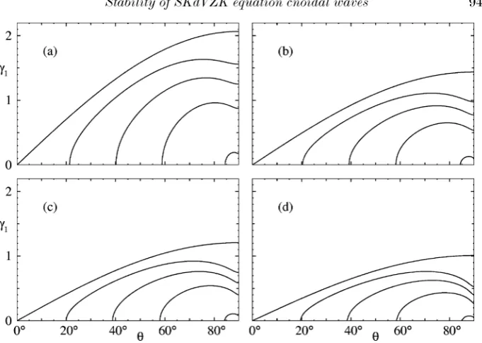
Figure 3.Plots ofγ1 againstθ for type I solutions withV = 4andctaking the values0 (top curves),−0.25,−0.5,−0.75and−0.99(lowest curves): (a)b= 0; (b)b= 2; (c)b= 4; (d)b= 50.

were checked using a finite-part numerical integration technique (O’Keir 1993; Phibanchon 2006).

4. Growth rate of instabilities

Having obtained the three roots to the nonlinear dispersion relation (3.20), we discard the real parts as they are of no importance in the context of stability. The solution is unstable if two of the roots are complex conjugates. Ifω1 is one of these

roots, the first-order growth rate of the instability is given by γ≡γ1k≡ |Imω1|k.

When examining the dependence of the growth rate on the type of solution and the direction of the perturbation we find it convenient to introduce the parameter c, a rescaled version ofC, defined by

c≡ C

|h(r+)|

, (4.1)

provided thatV >−6b2_{/25. Then, ifV >0, the linear limit corresponds toc=−1}

and the soliton limit occurs atc= 0. The type Ipeand IIpesolutions havec >0. As

in Part 1, we only consider the stability of solutions for whichb > 0as these are the more physically relevant.

We feel that a plot ofγ1 againstθshows the angular dependence of the growth

rate more clearly than the more traditional approach of using a polar plot to depict the dependence of the real and imaginary parts of ω at all angles. The values of γ1 for type I solution instabilities as a function of angle for a number of values of

Figure 4.Plots ofθm a x(solid lines),θcrit(dashed lines) andθc(dotted lines) againstc: (a)V = 4

withbtaking the values0(top curves),2,4and50(lowest curves); (b)V =−4withbtaking the values5(outermost curves),10and20(innermost curves).

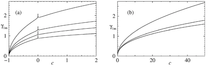
Figure 5.Plots ofγ1magainstc: (a)V = 4withbtaking the values0(top curves),2,4and

50(lowest curves)—dots indicate the values ofγ1 calculated for solitary wave solutions in Part 1; (b)V =−4withbtaking the values5(top curves),10and20(lowest curves).

is proportional tosinθ, which is in agreement with the results of Part 1. For the cnoidal wave solutions (when −1 < c < 0), γ1 is only non-zero above a critical

angle,θcrit, which increases with decreasingc. It is also evident thatθm ax, the angle

at which the maximum growth rate occurs, differs from90◦for cnoidal waves. The variation of both θm ax and θcrit with c is shown in Fig. 4(a). The growth rate is

largest for the soliton limit. From the plot ofγ1m, the maximum value ofγ1 (the

value whenθ=θm ax), in Fig. 5(a), it is apparent that there is a rapid variation in

growth rate ascapproaches zero. This is not unexpected given that the waveform period increases rapidly and becomes infinite at the soliton limit,c= 0. Notice that the results found for the soliton limit are in agreement with the analytical results given in Part 1 of this study.

In Part 1 it was found thatγ1 for solitary waves decreases with increasingbfor

a fixed value ofη. As is apparent from (2.2) of Part 1, for fixed η, the amplitude decreases asbincreases. However, if the amplitude is fixed (by using the appropriate value ofηin each case) then it is found thatγ1 increases withb. Cnoidal waves for

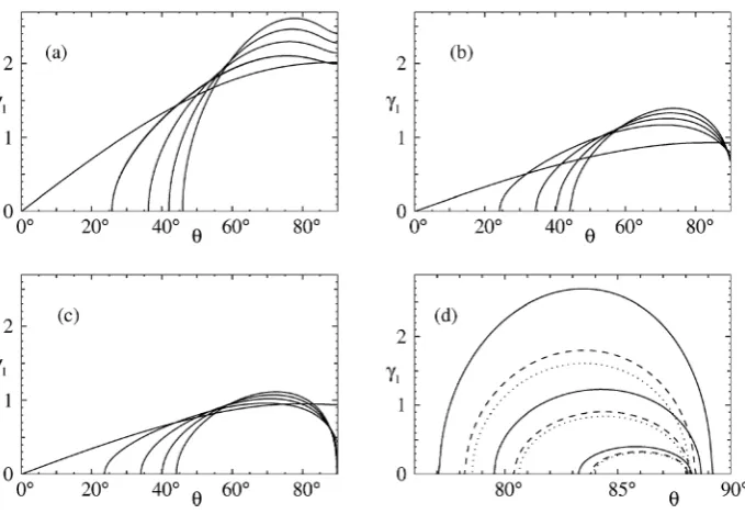
Figure 6.Plots ofγ1 againstθfor type IIpeand Ipesolutions. In (a)–(c),V = 4andctakes

the values0(leftmost curves),0.5,1.0,1.5and2.0(rightmost curves) and (a)b= 0, (b)b= 4, (c)b= 50. In (d)V = −4andctakes the values50(top curves),10and1(lowest curves) withb= 5(solid lines),b= 10(dashed lines) andb= 20(dotted lines).

and the plots in Fig. 4(a) indicate thatθm ax deviates from the perpendicular most

of all whenbis large. On the other hand,θcritshows only a slight dependence onb.

We now turn to the stability results for solutions in the form of functions extended by periodicity. When V > 0 and c is increased above zero, one obtains type IIpe

solutions. It can be seen from Figs 6(a)–(c) that the first-order growth rates of these solutions are higher than that for the soliton limit at some angles, but this range of angles decreases with increasingb. In addition to an increasingθcrit with

c, the first-order growth rate for exactly perpendicular perturbations vanishes for large enoughbandc. Evidently the growth rate has a significantly greater angular dependence than for the type I solutions.

For the stability results we have examined so far, the first-order growth rate is non-zero for angles just below90◦. In the case of type Ipeand IIpesolutions when

V <0the results in Fig. 6(d) indicate that there is a cut-off angleθcabove whichγ1

vanishes. Hence such waves are, to first order, stable to perpendicular perturbations. In addition, the instability occurs over a relatively small range of angles, even for large values ofc. For these types of solution, as is shown in Fig. 5(b), the growth rate increases monotonically withc, in contrast to the behaviour near the type I to type IIpetransition. There is no spike in the growth rate atc= 1, the type Ipe–IIpe

transition, since there is no sudden change of period around that point.

5. Conclusions

magnetized plasma with slightly non-isothermal electrons. It was found that the growth rate of instabilities for ordinary cnoidal waves that travel faster than long-wavelength linear waves has a stronger angular variation as the distribution of electrons becomes increasingly flatter than the isothermal Maxwellian. We also examined a class of solutions that do not occur for equations without a square root term. These solutions, which are written as functions extended by periodicity, have a minimum value of zero. This causes difficulties with some instances of recursion relations used in the determination of the growth rate, and results in it being necessary to evaluate an additional integral. This type of solution, for the case when the wave velocity is less than that of long-wavelength linear waves, has, to first order, a relatively narrow range of perturbation angles at which instability occurs and is stable to perpendicular perturbations.

The half-integer nonlinear term in the SKdVZK equation was originally intro-duced by Schamel to model the effect of trapped particles in Bernstein–Greene– Kruskal (BGK) solutions of the Vlasov–Poisson equation. Hence Part 1 and this paper are to be viewed as a step towards the more formidable problem of studying the stability of the BGK modes where trapped particles play a significant role. Acknowledgements

The authors wish to gratefully acknowledge support from the Thai Research Fund (PHD/47/2547). The first and second authors also wish to thank Warwick Univer-sity for its hospitality during their visits.

Appendix A. The evaluation of

α

,

α

and

α

For cnoidal wave solutions,α1/2, α1 and α3/2 are elliptic integrals and for their

evaluation we therefore rely heavily on the work of Byrd and Friedman (1954) to which the result numbers in the following refer.

A.1. Type I solutions

The type I solution as given by (2.5) has a period of2K(m)/η, whereK(m)is the complete elliptic integral of the first kind. From result 340.01 we obtain

α1/2 =r1+ (r4−r1)

Π(−ρ|m)

K(m) , (A 1)

in whichΠ(n|m)is the complete elliptic integral of the third kind. Applying result 340.02 to (2.5) yields

α1 =

(r4−r1)2

2(ρ+ 1)(1 +m)

ρE(m) +{ρ2_{+ 2ρ(1 +m) + 3m}Π(−ρ|m)}

K(m) −ρ−m

+r21+ 2r1(r4−r1)

Π(−ρ|m)

K(m) , (A 2)

whereE(m)is the complete elliptic integral of the second kind. A.2. Type IIpesolutions

After introducing σ=A−B

A+B, σ1 =

Arl−Bru Arl+Bru

, I¯n =

χ¯

0

dX

the integralsαn /2 forn= 1,2,3may be written in the form

αn /2 =

1 ¯

χ

Arl−Bru

A−B

nn

p= 0

n p

(σ/σ1−1)pI¯p.

From result 341,

¯

I1 =

1 1−σ2

Π(−q; ¯φ|m¯) +σ

µtan

−1_{[µsd( ¯χ|m¯)]}

, (A 3)

whereq=σ2_/(1−σ2_),φ¯_{=am( ¯χ|m¯),µ=}√_{m¯ +q, sd(x|m)≡sn(x|m)/dn(x|m),} ¯

I2= {

2 ¯m−(2 ¯m−1)σ2_}I¯

1+σ2E( ¯φ|m¯)− {m¯ + (1−m¯)σ2}χ¯+ ¯Υ1

(1−σ2₎{_{m¯ + (1}−_m¯)σ2} ,

¯

I3 =

3{2 ¯m−(2 ¯m−1)σ2_}I¯

2+ 2 ¯mF( ¯φ|m¯)− {6 ¯m−(2 ¯m−1)σ2}I¯1+ ¯Υ2

2(1−σ2₎{_{m¯ + (1}−_m¯)σ2} ,

whereF(φ|m)is the elliptic integral of the first kind, and

¯ Υn =

σ3_{sn( ¯χ|m¯)dn( ¯χ|m¯)}

(1−σcn( ¯χ|m¯))n−1.

A.3. TypeIpesolutions

Theαn /2 forn= 1,2,3may be written in the form

αn /2 =

rn

1

χ

n

p= 0

n p

(r4/r1−1)pIp,

where

In =

χ

0

dX

(1 +ρsn2_(X|_m))n.

From result 400.01, I1 = Π(−ρ;φ|m), where φ = am(χ|m). Results 336.01 and

336.02 yield I2 =

σE(φ|m)−(m+ρ)χ+{2ρ(1 +m) + 3m+ρ2_}I 1+ Υ1

2(1 +ρ)(m+ρ) , (A 4)

I3 =

mF(φ|m)−2{ρ(1 +m) + 3m}I1+ 3{2ρ(1 +m) + 3m+ρ2}I2+ Υ2

4(1 +ρ)(m+ρ) , (A 5)

respectively, where

Υn =ρ

2_{sn(χ|m)cn(χ|m)dn(χ|m)}

(1 +ρsn2_(χ|_m))n .

References

Allen, M. A., Phibanchon, S. and Rowlands, G. 2006 J. Plasma Phys. Published online 23 May 2006, doi:10.1017/S0022377806004508.

Byrd, P. F. and Friedman, M. D. 1954 Handbook of Elliptic Integrals for Engineers and Physicists. Berlin: Springer.

Infeld, E. 1985J. Plasma Phys.33, 171.

Munro, S. and Parkes, E. J. 1999J. Plasma Phys.62, 305.

O’Keir, I. S. 1993 The stability of solutions to modified generalized Korteweg–de Vries, nonlinear Schr¨odinger and Kadomtsev–Petviashvili equations. PhD thesis, University of Strathclyde.

O’Keir, I. S. and Parkes, E. J. 1997Phys. Scripta55, 135. Parkes, E. J. 1993J. Phys. A: Math. Gen.26, 6469.

Phibanchon, S. 2006 Nonlinear waves in plasmas with trapped electrons. PhD thesis, Mahidol University.

Rowlands, G. 1969J. Plasma Phys.3, 567. Schamel, H. 1972Plasma Phys.14, 905. Schamel, H. 1973J. Plasma Phys.9, 377.