Numerical analysis of an inverse problem for the eikonal equation

Original citation:

Deckelnick, Klaus, Elliott, Charles M. and Styles, Vanessa. (2011) Numerical analysis of an inverse problem for the eikonal equation. Numerische Mathematik, Vol.119 (No.2). pp. 245-269. ISSN 0029-599X

Permanent WRAP url:

http://wrap.warwick.ac.uk/39075

Copyright and reuse:

The Warwick Research Archive Portal (WRAP) makes the work of researchers of the University of Warwick available open access under the following conditions. Copyright © and all moral rights to the version of the paper presented here belong to the individual author(s) and/or other copyright owners. To the extent reasonable and practicable the material made available in WRAP has been checked for eligibility before being made available.

Copies of full items can be used for personal research or study, educational, or not-for-profit purposes without prior permission or charge. Provided that the authors, title and full bibliographic details are credited, a hyperlink and/or URL is given for the original metadata page and the content is not changed in any way.

Publisher’s statement:

First published in Numerische Mathematik by Springer. The final publication is available at link.springer.com

http://dx.doi.org/10.1007/s00211-011-0386-z

A note on versions:

The version presented here may differ from the published version or, version of record, if you wish to cite this item you are advised to consult the publisher’s version. Please see the ‘permanent WRAP url’ above for details on accessing the published version and note that access may require a subscription.

Numerical analysis of an inverse problem for the eikonal

equation

Klaus Deckelnick∗, Charles M. Elliott†and Vanessa Styles‡

Abstract

We are concerned with the inverse problem for an eikonal equation of determining the speed function using observations of the arrival time on a fixed surface. This is formulated as an optimisation problem for a quadratic functional with the state equa-tion being the eikonal equaequa-tion coupled to the so–called Soner boundary condiequa-tion. The state equation is discretised by a suitable finite difference scheme for which we obtain existence, uniqueness and an error bound. We set up an approximate optimi-sation problem and show that a subsequence of the discrete mimina converges to a solution of the continuous optimisation problem as the mesh size goes to zero. The derivative of the discrete functional is calculated with the help of an adjoint equation which can be solved efficiently by using fast marching techniques. Finally we describe some numerical results.

AMS:49J20, 49L25, 49M25

1

Introduction

Let Ω ⊂ _Rn _{be an open bounded domain with a Lipschitz boundary Γ and x}

0 ∈ Ω be

fixed. For a continuous, positive function a : ¯Ω → R and x ∈ Ω, x¯ 6= x0 we consider the

minimisation problem

inf{

Z 1

0

a(ξ(r))|ξ0(r)|dr|ξ∈W1,∞([0,1],Ω), ξ(0) =¯ x0, ξ(1) =x}. (1.1)

Its optimal value, u(x), gives the shortest travel time of the path connecting x0 to x in

¯

Ω with underlying velocity c(x) = _a(1_x). An important problem in various applications,

∗

Institut f¨ur Analysis und Numerik, Otto-von-Guericke-Universit¨at Magdeburg, Universit¨atsplatz 2, 39106 Magdeburg, Germany.

†

Mathematics Institute, University of Warwick, Coventry CV4 7AL, UK.

‡

e.g. tomography, consists in reconstructing the slowness function a from measured first arrival times on a suitable subset of Γ. A common approach to solve this inverse problem aims at minimising the misfit between the measured data and computed traveltimes, that are obtained from integrating the Euler-Lagrange equation corresponding to (1.1), see e.g. [6, 19]. A more recent approach, see e.g. [13], makes use of the fact that the optimal value function for (1.1) formally is a solution of the following eikonal equation, see [12],

|∇u|=a(x), x∈Ω\ {x0}; (1.2)

with boundary conditions

u(x0) = 0, (1.3)

∇u(x)·ν(x) ≥ 0, x∈Γ. (1.4)

Here,νis the unit outer normal to Γ. The condition (1.4) is a consequence of the definition, (1.1), of the first arrival time,u(x), at a pointx∈Ω which constrains paths from the source¯ to the arrival point,x, to lie in ¯Ω. Informally observe that the gradient of the first arrival time for an optimal path is in the tangential direction of the path and on the boundary Γ the tangent to this path, which is constrained to lie in ¯Ω, has a non-negative component in the outward pointing normal direction.

It can be shown that the above problem has a unique Lipschitz continuous solutionu=ua

that satisfies (1.2), (1.3) and (1.4) in the viscosity sense, see Section 2. Let us return to the abovementioned inverse problem and assume that the measured arrival times are given by a functionuobs : Γ→R>0. Then, the misfit functional takes the form

J(a) = 1 2

Z

Γ

|ua(x)−uobs(x)|2dox (1.5)

which needs to be minimised over a suitable set K of slowness functions. The functional (1.5) may be generalised by considering several source points xj₀, j = 1, . . . , S with first arrival timesuj_obs : Γ→R>0 resulting in

J(a) = 1 2

S

X

j=1

Z

Γ

|uj_a(x)−uj_obs(x)|2dox. (1.6)

The above approach has been studied numerically in the context of tomography in [11, 17, 18] using finite difference approximations of the eikonal equation and fast sweeping methods for solving the forward equation and the adjoint equation. The aim of the present work is to present a corresponding numerical analysis. Let us outline the contents of this paper and our contributions.

boundary condition. In Section 3 we discretize (1.2)–(1.4) with the help of a monotone finite difference scheme. We show existence and uniqueness of the discrete solution and derive an O(h12) error bound, which appears to be new for a Hamilton–Jacobi equation coupled to the Soner boundary condition. The discrete solution is computed with the help of the fast marching method and we show that the procedure terminates in a finite number of cycles. In Section 3 we address the problem of approximating the functional (1.5). We assume that the setKof admissible slowness functions consists of continuous functions that are finite linear combinations of a given partition of unity. Replacing ua in (1.5) by the

discrete solution gives rise to an approximate minimisation problem, which is shown to have a solution. We then prove that a subsequence of the discrete minima converges to a solution of the continuous minimisation problem. In practice, the discrete optimisation problem is solved by a descent method and the derivative of the discrete functional is calculated with the help of a discrete adjoint equation. In order to be able to derive this equation we require differentiability of the discrete state with respect to the slowness function which is ensured by a suitable choice of the finite difference scheme. We then show that the discrete adjoint equation has a unique solution. Furthermore, when the solution of the state equation has been computed by fast marching, the resulting ordering of grid values can be used in order to efficiently compute the adjoint solution without solving an equation. In Section 4 we finally present a series of numerical tests in which we consider the more general functional (1.6) and apply our discretization strategy to varying geometries and numbers of degrees of freedom fora. Let us finish this introduction by referring to [5, 9], where optimal control problems for time dependent Hamilton-Jacobi equations were considered.

2

Wellposedness and approximation of the state equation

2.1 Existence and uniqueness

Definition 2.1. A functionu∈C0(Ω) is called a viscosity subsolution of (1.2) in Ω\ {x0}

if for each ζ∈C∞(Ω): if u−ζ has a local maximum at a pointx∈Ω\ {x0}, then

|∇ζ(x)| ≤a(x).

A function u ∈ C0( ¯Ω) is called a viscosity supersolution of (1.2) in ¯Ω\ {x0} if for each

ζ ∈C∞(Rn): ifu−ζ has a local minimum at a pointx∈Ω¯\ {x0}, relative to ¯Ω, then

|∇ζ(x)| ≥a(x).

A viscosity solution of (1.2), (1.3), (1.4) is then a functionu∈C0( ¯Ω) which is a viscosity subsolution in Ω\ {x0}, a viscosity supersolution in ¯Ω\ {x0}and which satisfiesu(x0) = 0.

interpretation of the boundary condition (1.4). This kind of condition, also referred to as Soner boundary condition, is relevant in optimal control problems with constraints on the state variable, cf. [16], [7].

In what follows we shall assume the following regularity condition on Ω, cf. [16], [3], p. 278: there exists a continuous functionη : ¯Ω→Rn and >0 such that

Bs(x+sη(x))⊂Ω for allx∈Ω,¯ 0< s≤. (2.1)

Theorem 2.2. Suppose that a ∈ C0( ¯Ω) is positive. Then there exists a unique viscosity solution u∈C0( ¯Ω) of (1.2)–(1.4). The solution is given by the formula

u(x) = inf{

Z 1

0

a(ξ(r))|ξ0(r)|dr|ξ ∈W1,∞([0,1],Ω), ξ(0) =¯ x0, ξ(1) =x}.

Furthermore, there exists a constant C = C(Ω) such that u is Lipschitz continuous in Ω

with an upper bound on the Lipschitz constant satisfying

lip(u)≤Cmax

¯

Ω a. (2.2)

Proof.See [16], [7].

2.2 Discretization of the state equation

The numerical solution of the boundary value problem (1.2)–(1.4) in the context of geo-physical applications was considered in [4, 2, 1]. In particular, in [1] this problem is solved by time stepping on unstructured triangular grids. We shall use a finite difference method which is set up in such a way that the solution is differentiable with respect to the slow-ness function. In order to keep the exposition simple we consider the two–dimensional case although our arguments can be generalized to higher dimensions.

Let us assume that Ω⊂_R2 _{has a boundary Γ which is piecewise C}2_{. Forh > 0 consider}

the regular grid

Z2h :={xα = (hα1, hα2)|αi ∈Z, i= 1,2}.

We suppose for simplicity thatx0 is a grid point, say x0 =xα0 for some α0 ∈Z

2_{. Next, let}

Ωh= Ω∩Z2h be the set of inner grid points. If for somexα∈Ωh there are σ∈ {−1,1}, k∈

{1,2} with xα+σek ∈/ Ω, then there exists s∈ (0,1] such that xα+sσhek ∈Γ and we set β:=α+sσek as well as xβ :=xα+sσhek∈Γ. We denote by Γh⊂Γ the set of all points

obtained in this way and defineGh := Ωh∪Γh. For a point xα∈Gh we let

Nα:=







{xβ ∈Gh|xβ is a neighbour ofxα}, xα∈Ωh

Note that forxα ∈Γh the setNα only comprises the interior neighbours.

We approximate the solution of (1.2)–(1.4) by a function U :Gh →Ras follows:

Uα0 = 0, (2.3)

X

xβ∈Nα

Uα−Uβ

hαβ

+2

= a(xα)2, xα∈Gh\ {xα0}. (2.4)

Here we have abbreviatedUα=U(xα) and hαβ =|xα−xβ|.

Lemma 2.3. Suppose thata∈C0( ¯Ω)is positive. Then, (2.3), (2.4) has a unique solution

U :Gh →Rand

(a)Uα ≥0, xα∈Gh;

(b)|Uα−Uβ| ≤Cmax

¯ Ω

a|xα−xβ|, xα, xβ ∈Gh,

where the constantC is independent of h.

Proof.We start by sketching the proof for the existence of a discrete solution, compare [8] for similar arguments. Note first that the functionZ :Gh →R, Zα:=M|xα−xα0|satisfies Zα0 = 0 as well as

X

xβ∈Nα

Zα−Zβ

hαβ

+2

≥a(xα)2, xα ∈Gh\ {xα0}, (2.5)

provided thatM is chosen sufficiently large. We now consider the following iteration: Set U0:=Z and givenUk :Gh→R≥0 define Uk+1:Gh →R≥0 by Uαk+10 = 0 and

U_αk+1 := inf

t≥0| X

xβ∈Nα

t−U

k β

hαβ

+2

≥a(xα)2 , xα ∈Gh\ {xα0}.

An induction argument based on (2.5) and the monotonicity of the scheme shows that (U_αk)k∈_N is decreasing for allxα ∈Gh, so thatUα := limk→∞Uαk exists for all xα ∈Gh. It

is not difficult to verify thatU is indeed a solution of (2.3), (2.4).

In order to prove uniqueness, let us suppose thatU,U˜ :Gh →Rare two solutions of (2.3), (2.4). We set

µ:= max

xα∈Gh

(Uα−U˜α)

and suppose that µ > 0. There exists a pointxγ ∈Gh\ {xα0} with Uγ−U˜γ = µ. Let us introduce W : Gh → R by Wα := ˜Uα+µ, xα ∈ Gh. Clearly, Wα ≥ Uα, xα ∈ Gh, while

Wγ =Uγ. Hence,

As a consequence,

X

xβ∈Nγ

U˜γ−U˜β

hγβ

+2

= X

xβ∈Nγ

Wγ−Wβ

hγβ

+2

≤ X

xβ∈Nγ

Uγ−Uβ

hγβ

+2

.

SinceU and ˜U are both solutions we deduce from the above relation that

a(xγ)2 =

X

xβ∈Nγ

Uγ−Uβ

hγβ

+2

= X

xβ∈Nγ

Wγ−Wβ

hγβ

+2

.

Recalling (2.6) and observing thata(xγ)2 >0 we infer that there exists xβ ∈ Nγ such that

0< Wγ−Wβ =Uγ−Uβ,

and therefore

Uβ−U˜β =µ and Uβ < Uγ. (2.7)

We can now repeat the above argument withγreplaced byβgenerating a sequence of points which satisfy (2.7). Since the values of U are strictly decreasing, every point appears only once, so that necessarilyxα0 will eventually be crossed contradicting (2.3). Henceµ≤0, so thatUα≤U˜α, xα ∈Gh. Exchanging the roles ofU and ˜U we infer thatUα = ˜Uα, xα∈Gh.

From the positivity of aand the definition of the scheme it is straightforward to see that the minimum of U cannot be attained at a point xα 6=xα0, so that min

xα∈Gh

Uα = Uα0 = 0

proving (a).

In order to show (b) we first note that (2.4) together with the fact that xβ ∈ Nα if and

only if xα∈ Nβ implies that

|Uα−Uβ| ≤max_¯

Ω a

|xα−xβ| (2.8)

for all grid pointsxα, xβ ∈Gh that are neighbours of each other. In order to estimate the

above difference for arbitrary pairsxα, xβ ∈Gh we first extendU to a function ˆU : ¯Ω→R as follows: The gridZ2h gives rise to a partition of ¯Ω into squares that are possibly truncated

near the boundary. A square Q that lies entirely in ¯Ω is divided into two triangles along its diagonal and ˆU is defined by linear interpolation, so that |∇Uˆ|Q| ≤max_Ω¯ ain view of

(2.8). A truncated square Q at the boundary can also be subdivided into triangles with possibly one curved edge and again ˆU is defined via linear interpolation. It can be shown that this can be done in such a way that|∇Uˆ|Q| ≤ 3 max_Ω¯a. Thus we obtain a function

ˆ

U ∈ W1,∞(Ω) with |∇Uˆ| ≤3 max_Ω¯a a.e. in Ω. Making use of the continuous embedding

W1,∞(Ω),→C0,1( ¯Ω) we finally obtain for arbitrary xα, xβ ∈Gh

|Uα−Uβ|=|Uˆ(xα)−Uˆ(xβ)| ≤Ck∇UˆkL∞|x_α−x_β| ≤Cmax

¯ Ω

a|xα−xβ|,

2.3 Construction of a solution by the fast marching method

A solution to (2.3), (2.4) can be found efficiently, without iteration, using the fast marching procedure, see [14], [15]. Recall that the idea behind this method is that the unique solution Uα of (2.3), (2.4) at a grid point xα only depends on neighbouring values Uβ such that

0≤Uβ < Uα so that the solution can be obtained in increasing order of magnitude of the

grid valuesUα. Solving the equation then becomes an issue of sorting the grid values.

In particular the following algorithm is used: First tag xα0 as knownand tag as trial all points that are one grid point away from thisknownpoint. Finally tag asf arall remaining points. Now cycle through the followingFast Marching Procedure:

Step 1 Compute a trial value of ˜Uα for everyxα ∈trial according to (2.4) assuming that

it is smaller than or equal to itstrial neighbours.

Step 2 Let xµ be any trial point such that the trial values satisfy ˜Uµ ≤U˜α for all xα ∈

trial.

Step 3 Set Uµ= ˜Uµ for all such xµ and add xµ toknownand remove fromtrial.

Step 4 Tag all neighbours of knownastrial if they are notknown.

Step 5 If trial={∅}then STOP.

Step 6 Return to Step 1.

Lemma 2.4. The Fast Marching Procedure terminates in K cycles whereK is the number of distinct positive values taken by the solution U of Lemma 2.3.

Proof. Let us denote by 0 = V0 < V1 < V2 < . . . VK the K+ 1 distinct values taken by

U and define Em := {xα ∈ Gh|Uα = Vm},0 ≤ m ≤ K. The lemma is proved once we

can show that E0∪. . .∪Em coincides with the set of known points after m cycles. This

is certainly true for m = 0. Now suppose that this claim holds for some 0 ≤ m < K, so that the known points after m cycles are given by E0 ∪. . .∪Em. Let xα ∈ trial and

Nm,α=known∩ Nα. We denote byr >minxβ∈Nm,αUβ the unique solution of the equation

X

xβ∈Nm,α

r−Uβ

hαβ

+2

=a(xα)2 (2.9)

and suppose that r ≤maxxβ∈Nm,αUβ. Then there would be xβ1, xβ2 ∈ Nm,α with Uβ1 < r≤Uβ2, sayxβ1 ∈El, xβ2 ∈Ek, l < k≤m. But then the valuer will have been computed as a trial value in the k–th cycle. Since xα has not been added to known we must have

r > Vk=Uβ2, a contradiction. Hencer >maxxβ∈Nm,αUβ and in view of (2.4) the smallest of the trial values satisfying (2.9) is given byVm+1. As the points xα that take this value

are added toknown the induction step is finished.

2.4 Error estimate

Theorem 2.6. Suppose that a : ¯Ω → R is Lipschitz continuous and satisfies 0 < Am ≤

a(x)≤AM for allx∈Ω¯. Let u be the viscosity solution of (1.2)–(1.4) and U the solution of (2.3), (2.4). Then there existsh0>0 such that for all 0< h≤h0

max

xα∈Gh

|u(xα)−Uα| ≤C

√

h. (2.10)

The constantsh0 and C depend on Ω,Am, AM,lip(a) and the functionη from (2.1). Proof.Let >0 be the constant in (2.1). Since ηis uniformly continuous on ¯Ω, there exists δ >0 such that

|η(x)−η(y)|<

2 for allx, y∈Ω with¯ |x−y|< δ. (2.11)

Denoting by lip(u) the Lipschitz constant of u and by lip(U) the constant appearing in Lemma 2.3(b) we set

R :=

r

(lip(u))2₊ 1

2 lip(u)

2_{+ lip(U)}2

+ max

¯ Ω

|η|2_{. (2.12)}

Let us chooseL≥1, M ≥1 so large that

√

2R

√

L ≤ 4,

R

√

M ≤ δ

2. (2.13)

Note thatR and hence also L and M only depend on Ω and AM in view of Theorem 2.2

and Lemma 2.3. We first estimate max

xα∈Gh

(u(xα)−Uα). Choosexγ ∈Gh such that

max

xα∈Gh

(1−ρ√h)u(xα)−Uα

= (1−ρ√h)u(xγ)−Uγ. (2.14)

Here, the constantρ will be chosen later and we takeh0>0 so small that

1−ρph0≤1 andh0≤2. (2.15)

The factor (1−ρ√h) in (2.14) is motivated by Ishii’s uniqueness proof for Hamilton–Jacobi equations of eikonal type, see [10]. We now employ the usual doubling of variables technique and define Φ : ¯Ω×Gh →R by

Φ(x, xα) := (1−ρ

√

h)u(x)−Uα−

L

√

h|x−xα−

√

hη(xγ)|2−M

√

h|xα−xγ|2.

There exists (xh, xαh)∈Ω¯ ×Gh such that

Φ(xh, xαh) = max

(x,xα)∈Ω¯×Gh

Our goal will be to show that for a suitable choice of ρ at least one of the points xh or

xαh has to coincide with the source point x0 and then to use that u(x0) =U(x0) = 0. In order to exclude the possibility that bothxh andxαh are different fromx0 we will employ among other things the fact thatu is a viscosity subsolution at xh. However, this is only

possible provided we can ensure thatxh does not belong to the boundary of Ω (compare

Definition 2.1). This will be accomplished with the help of the shift√hη(xγ) in the third

term of Φ, an idea going back to Soner, [16].

Let us now carry out the proof in detail. In view of (2.1) and (2.15) we have that xγ +

√

h η(xγ)∈Ω for 0< h≤h0 and hence

Φ(xh, xαh)≥Φ(xγ+

√

h η(xγ), xγ),

or equivalently

(1−ρ

√

h)u(xh)−Uαh− L

√

h|xh−xαh−

√

h η(xγ)|2−M

√

h|xαh−xγ|

2

≥ (1−ρ

√

h)u(xγ+

√

h η(xγ))−Uγ. (2.16)

Using (2.14) we obtain

L

√

h|xh−xαh−

√

h η(xγ)|2+M

√

h|xαh−xγ|

2 _(2.17)

≤ (1−ρ

√

h)u(xh)−Uαh−(1−ρ

√

h)u(xγ+

√

h η(xγ)) +Uγ

= (1−ρ

√

h)u(xαh)−Uαh− (1−ρ

√

h)u(xγ)−Uγ

+(1−ρ√h)u(xh)−(1−ρ

√

h)u(xαh) + (1−ρ

√

h) u(xγ)−u(xγ+

√

h η(xγ))

≤ lip(u) |xh−xαh|+

√

hmax

¯ Ω

|η|

≤ lip(u) |xh−xαh−

√

h η(xγ)|+ 2

√

hmax

¯ Ω

|η|

≤ L

2√h|xh−xαh−

√

h η(xγ)|2+

√

h 3

2(lip(u))

2_{+ max} ¯ Ω

|η|2

.

Recalling (2.12) and (2.13) we obtain that

|xh−xαh−

√

h η(xγ)| ≤

√ 2R √ L √ h≤ 4 √ h < 2 √ h (2.18)

|xαh−xγ| ≤ R

√

M ≤ δ

2 < δ. (2.19)

In particular, (2.18), (2.19) and (2.11) imply that

|xh−xαh−

√

h η(xαh)| ≤ |xh−xαh−

√

h η(xγ)|+

√

h|η(xαh)−η(xγ)|

Hencexh ∈B√_h(xαh+

√

h η(xαh))⊂Ω for 0< h≤h0 by (2.1). We distinguish two cases:

Case 1:xh ∈Ω\ {x0} andxαh ∈Gh\ {x0}. Noting that

x7→u(x)− L

(1−ρ√h)√h|x−xαh−

√

hη(xγ)|2

has a maximum atx=xh we obtain from the fact that uis a viscosity subsolution that

2L

(1−ρ√h)√h|xh−xαh−

√

hη(xγ)| ≤a(xh). (2.20)

On the other hand, observing that Φ(xh, xαh)≥Φ(xh, xα), xα∈Gh we obtain

Uα ≥Uαh+ L

√

h{|xh−xαh−

√

h η(xγ)|2− |xh−xα−

√

h η(xγ)|2}

+M√h{|xαh−xγ|

2_{− |x}

α−xγ|2} =: Vα.

A short calculation shows that for xβ ∈ Nα

Vα−Vβ =−

2L

√

h xh−xα−

√

h η(xγ), xβ−xα

+rαβ

where

rαβ =

L

√

h|xβ−xα|

2_+M√_{h x}

β−xα, xβ+xα−2xγ

.

Hence,

|Vα−Vβ

hαβ

| ≤ √2L

h| xh−xα−

√

h η(xγ),

xβ−xα

hαβ

|+C1

√

h, xβ ∈ Nα (2.21)

where the constantC1 only depends on L, M and Ω.

Next, sinceUα≥Vα, xα ∈Gh,Uαh =Vαh we have

Uαh−Uβ ≤Vαh−Vβ, xβ ∈ Nαh.

We deduce from (2.4) and (2.21)

a(xαh) =

_X

xβ∈Nαh

Uαh−Uβ

hαhβ

+2

1 2

≤ X

xβ∈Nαh

Vαh−Vβ

hαhβ

+2

1 2

≤ √2L

h|xh−xαh−

√

h η(xγ)|+C2

√

whereC2 depends on the same quantities as C1. Combining (2.20) and (2.22) we have

2L

√

h|xh−xαh−

√

hη(xγ)| ≤(1−ρ

√

h)a(xh)

≤ (a(xh)−a(xαh)) +a(xαh)−ρ

√

h a(xh) (2.23)

≤ lip(a)|xh−xαh|+ 2L

√

h|xh−xαh−

√

h η(xγ)|+C2

√

h−ρAm

√

h.

Furthermore, (2.18) implies that

|xh−xαh| ≤ |xh−xαh−

√

h η(xγ)|+ max

¯ Ω

|η|√h≤

2+ max_Ω¯ |η|

√

h,

which together with (2.23) yields

0≤ C2−ρAm+ lip(a)(

2 + max_Ω¯ |η|)

√

h <0

a contradiction, if we choose for example ρ = C2+lip(a)(

2+maxΩ¯|η|)

Am + 1. Hence this case cannot occur and we note thatρ only depends on Ω, Am, AM, η and lip(a).

Case 2:xh =x0 orxαh =x0. We obtain from (2.16) and the fact thatUα≥0, u(x0) = 0 (1−ρ√h)u(xγ+

√

h η(xγ))−Uγ ≤(1−ρ

√

h)u(xh)−Uαh

≤ u(xh)≤min(u(xh), u(xαh)) + lip(u)|xh−xαh|

≤ lip(u)|xh−xαh−

√

h η(xγ)|+

√

hlip(u) max

¯ Ω

|η|

≤ lip(u)

2+ max_Ω¯ |η|

√

h

by (2.18). As a consequence, recalling the definition ofxγ

max

xα∈Gh

(u(xα)−Uα) ≤ (1−ρ

√

h)u(xγ)−Uγ+ρ

√

hmax

¯ Ω

u

≤ (1−ρ

√

h)u(xγ+

√

h η(xγ))−Uγ+ lip(u) max

¯ Ω

|η|√h+ρ

√

hmax

¯ Ω u

≤ C3

√

h, (2.24)

where C3 depends on the same quantities as ρ. Note that the bound on max_Ω¯u follows

from

u(x) =u(x)−u(x0)≤lip(u)|x−x0| ≤CAMdiam(Ω) (2.25)

in view of (1.3) and Theorem 2.2.

It remains to derive an upper bound on max

xα∈Gh

(Uα−u(xα)). This will be done in a similar

way as above and we will only sketch the argument. To begin, letxγ ∈Gh be such that

max

xα∈Gh

(1−ρ√h)Uα−u(xα)

and define Φ : ¯Ω×Gh →R by

Φ(x, xα) := (1−ρ

√

h)Uα−u(x)−

L

√

h|xα−x−

√

hη(xγ)|2−M

√

h|x−xγ|2.

There exists (xh, xαh)∈Ω¯×Gh such that Φ(xh, xαh) = max_¯

Ω×Gh

Φ. Since xγ+

√

h η(xγ)∈Ω

for 0< h≤h0 there existsxγ˜ ∈Gh with

|x˜γ−xγ−

√

h η(xγ)| ≤h. (2.26)

The inequality Φ(xh, xαh)≥Φ(xγ, x˜γ) together with (2.26) implies

(1−ρ√h)Uαh−u(xh)− L

√

h|xαh−xh−

√

h η(xγ)|2−M

√

h|xh−xγ|2

≥ (1−ρ

√

h)U˜γ−u(xγ)−Lh

3

2. (2.27)

We can argue as in (2.17) to show that

L

√

h|xαh−xh−

√

h η(xγ)|2+M

√

h|xh−xγ|2

≤ L

2√h|xαh−xh−

√

h η(xγ)|2+

√

h (lip(u))2+1 2lip(U)

2_{+ max} ¯ Ω

|η|2

+Lh32,

from which we conclude recalling (2.12)

|xαh−xh−

√

h η(xγ)| ≤

4

√

h+√2h < 2

√

h,

|xh−xγ| ≤

R

√

M + L

√

Mh≤ δ 2 +

L

√

Mh < δ

for 0 < h ≤ h0, where h0 is chosen smaller if necessary. Just as above we deduce that

xαh ∈B√h(xh+

√

h η(xh))⊂Ω for 0< h≤h1 and then rule out that xh ∈Ω¯ \ {x0} and

xαh ∈Ωh\ {x0} by choosingρ sufficiently large. It remains to consider the casexh =x0 or xαh =x0. Combining (2.27) with the fact that x0 =xα0 and Lemma 2.3(b) we have

(1−ρ√h)U˜γ−u(xγ)≤(1−ρ

√

h)Uαh−u(xh) +Lh 3 2 ≤U_α

h+Lh 3 2

≤ min(Uαh, Uα0) +CAM|xh−xαh|+Lh 3 2

≤ CAM|xαh−xh−

√

h η(xγ)|+CAMmax

¯ Ω

|η|√h+Lh32

≤ C4

√

h.

Hence, we finally have similarly as above

max

xα∈Gh

(Uα−u(xα))≤C5

√

h, (2.28)

where C5 again only depends on Ω, Am, AM, η and lip(a). The inequalities (2.24) and

3

The optimal control problem

3.1 The continuous problem

Let 0< Am < AM <∞ and the positive function uobs ∈C0,1(Γ) be given. We introduce

the set

K:={a: ¯Ω→_R|a(x) =

L

X

i=1

aiφi(x), Am ≤ai ≤AM,1≤i≤L}

where {φi}Li=1 satisfyφi ∈ W1,∞(D), φi(x) ≥ 0, i = 1, . . . , L and

PL

i=1φi(x) = 1, x∈ Ω,

¯

Ω⊂D=

L

[

i=1

supp(φi).

Given a∈ K we denote by u = ua the solution of (1.2)–(1.4) given by Theorem 2.2 and

consider the following optimal control problem

(P) min

a∈KJ(a) =

1 2

Z

Γ

|ua(x)−uobs(x)|2dox.

3.2 The discrete control problem

The aim of this section is to set up and analyze a discrete approximation of (P). We start by defining a suitable approximation of the integralR

Γ|ua(x)−uobs(x)|2dox. To this purpose

we choose an embedding γ : [0,1] → R2, which is piecewise C2 such that γ([0,1]) = Γ, γ(0) = γ(1) and |γ0(t)| ≥c0 >0, with the exception of finitely many t∈[0,1]. For every

xα ∈Γh there exists a unique tα∈[0,1] withγ(tα) =xα. Ordering the different preimages

in the form 0≤tα1 < tα2 < . . . < tαN <1 induces an ordering of the boundary grid points xαi =γ(tαi), i= 1, . . . , N. For each xα=xαi ∈Γh we let

hα:=

1

2 |xαi+1−xαi|+|xαi−xαi−1|

(3.1)

with the conventiontαN+1 =tα1, tα0 =tαN. Furthermore, choosing a sequence (δh)h>0with δh ≥0 and limh→0δh = 0 we approximate the functionalJ by

J_h(a) = 1 2

X

xα∈Γh

hα|Ua(xα)−uobs(xα)|2+

δh

2

Z

Ω

|∇a|2,

whereUa is the solution of (2.3), (2.4). Let us first establish the consistency of the above

approximation.

Lemma 3.1. Let a=PL

i=1aiφi∈K. Then

J_h(a)→ J(a), as h→0,

Proof. The assertion is a consequence of the following estimate which we will need again later on:

|1

2

X

xα∈Γh

hα|Ua(xα)−uobs(xα)|2−

1 2

Z

Γ

|ua(x)−uobs(x)|2dox| ≤C

√

h, (3.2)

where the constantC is independent ofa∈K. In order to prove (3.2) we write

1 2

X

xα∈Γh

hα|Ua(xα)−uobs(xα)|2−

1 2

Z

Γ

|ua(x)−uobs(x)|2dox

= 1 2

N

X

i=1

hαi

|Ua(xαi)−uobs(xαi)|

2_{− |u}

a(xαi)−uobs(xαi)|

2 +1 2 N X i=1

hαi|ua(xαi)−uobs(xαi)|

2₋

Z

Γ

|ua(x)−uobs(x)|2dox ≡ I+II.

Recalling Theorem 2.6 we have

|I| ≤ |Γ| max

xα∈Gh

|ua(xα)−Ua(xα)| max

¯

Ω ua+ maxGh

Ua+ 2 max

Γ uobs

≤C

√

h,

where the constantC is independent ofa∈K since lip(a)≤LAMmaxi=1,...,Lk∇φikL∞_(Ω) for alla∈ K. Note also that max_Ω¯ ua and maxGhUa can be bounded independently of a using the estimate (2.25) and a corresponding bound forUa.

Next, we have forfa(x) := 1₂|ua(x)−uobs(x)|2

II =

N

X

i=1

fa(xαi) 1

2 |γ(tαi+1)−γ(tαi)|+|γ(tαi)−γ(tαi−1)|

−

Z 1

0

fa(γ(t))|γ0(t)|dt

=

N

X

i=1

Z t_αi

+1

t_αi

1

2 fa(γ(tαi)) +fa(γ(tαi+1))

−fa(γ(t)) |γ0(t)|dt

+

N

X

i=1

1

2 fa(γ(tαi)) +fa(γ(tαi+1))

|γ(tαi+1)−γ(tαi)| −

Z t_αi+1

t_αi

|γ0(t)|dt ≡II1+II2.

Observing that ua and hence fa is Lipschitz on Γ with a constant that is independent of

a∈K we infer that|II1| ≤Ch. Furthermore, since γ is piecewiseC2 we also have

|

Z t_αi+1

t_αi

|γ0(t)|dt− |γ(tαi+1)−γ(tαi)|| ≤Ch(tαi+1−tαi),

which implies that|II2| ≤Ch. This proves (3.2) and the result follows from the fact that

We now consider the following discrete control problem:

(Ph) min

a∈KJh(a).

Theorem 3.2. The problem(Ph)has at least one solutiona∗_h∈K. There exists a sequence

h → 0 such that a∗_h → a∗ for some a∗ ∈ K and a∗ is a solution of (P). Furthermore, if

δh >0 for allh >0 and limh→0

√

h

δh = 0, then

Z

Ω

|∇a∗|2≤

Z

Ω

|∇a˜|2 for every solution ˜aof (P). (3.3)

Proof.It is not difficult to see that the mappinga7→Uais continuous and hence there exists

a minimizer a∗_h ∈K of (Ph). Furthermore, observing that Am ≤a∗h,i ≤AM, i= 1, . . . , L,

there exists a sequence h → 0 and a∗ ∈ K such that a∗_h → a∗ uniformly in ¯Ω. Let us abbreviate uh = ua∗

h, u =ua

∗. Standard stability arguments from the theory of viscosity solutions show thatuh →uuniformly in ¯Ω after possibly extracting a further subsequence. As a consequence,

lim

h→0J(a

∗

h) =J(a

∗

). (3.4)

Now, if a∈K is arbitrary we rewrite the relationJ_h(a∗_h)≤ J_h(a) as

J(a∗_h)≤ J_h(a) + J(a∗_h)− J_h(a∗_h).

Using (3.4) and Lemma 3.1 we deduce that a∗ solves (P) by passing to the limit h → 0. Finally, suppose that δh > 0, h >0 with limh→0

√

h

δh = 0 and that ˜a ∈ K is an arbitrary solution of (P). Rewriting the relation J_h(a∗_h)≤ J_h(˜a) we obtain

Z

Ω

|∇a∗_h|2 ≤

Z

Ω

|∇˜a|2+ 1 δh

X

xα∈Γh

hα|U˜a(xα)−uobs(xα)|2−

X

xα∈Γh hα|Ua∗

h(xα)−uobs(xα)|

2

≤

Z

Ω

|∇˜a|2+ 1 δh

X

xα∈Γh

hα|U˜a(xα)−uobs(xα)|2−

Z

Γ

|u˜a(x)−uobs(x)|2dox

+1 δh

Z

Γ

|ua∗

h(x)−uobs(x)|

2_do

x−

X

xα∈Γh hα|Ua∗

h(xα)−uobs(xα)|

2

,

sinceJ(˜a)≤ J(a∗_h). Recalling (3.2) we deduce that

Z

Ω

|∇a∗_h|2 ≤

Z

Ω

|∇˜a|2+C

√

h δh

3.3 The discrete adjoint equation

LetU :Gh→Rbe the solution of (2.3), (2.4). We introduce the following adjoint problem: Find P :Gh\ {xα0} →Rsuch that

X

xβ∈Nα

Uα−Uβ

hαβ

+ Pα

hαβ

− Uβ−Uα

hαβ

+ Pβ

hαβ

= 0, xα∈Ωh\ {xα0}; (3.5)

X

xβ∈Nα

Uα−Uβ

hαβ

+ Pα

hαβ

− Uβ−Uα

hαβ

+ Pβ

hαβ

= hα

h2 uobs(xα)−Uα

, xα∈Γh, (3.6)

wherehα is given by (3.1). Note that the fact thatP is not defined atxα0 does not cause a problem in evaluating (3.5). Ifxα0 ∈ Nαfor somexα∈Ωhthen

Uα₀−Uα

hαβ

+

= −Uα

hαβ

+

= 0.

Lemma 3.3. For a given function Q:Gh\ {xα0} →R there exists a unique V :Gh→R

withVα0 = 0 and

X

xβ∈Nα

Uα−Uβ

hαβ

+ Vα−Vβ

hαβ

=Qα, xα∈Gh\ {xα0}.

Proof.It is sufficient to check that the linear problem: Vα0 = 0 and

X

xβ∈Nα

Uα−Uβ

hαβ

+ Vα−Vβ

hαβ

= 0, xα∈Gh\ {xα0}

only has the trivial solution. Let us enumerate the grid points in such a way that 0 =Uα0 < Uα1 ≤Uα2 ≤. . .≤UαM where M+ 1 = |Gh|. Assume that Vα0 =Vα1 =. . .=Vαr−1 = 0 already holds for somer ∈ {1, . . . , M}. Then

0 = X

xβ∈Nαr

Uαr −Uβ hαrβ

+ Vαr−Vβ

hαrβ

=Vαr

X

xβ∈Nαr

Uαr −Uβ hαrβ

+ 1

hαrβ

since Vβ = 0 if Uβ < Uαr. Recalling (2.4) and the fact that a(xαr) > 0 we infer that Vαr = 0. By induction we then deduce thatV ≡0.

Lemma 3.4. Problem (3.5)–(3.6) has a unique solution P :Gh\ {xα0} →R.

Proof. Since the problem is linear it is sufficient to check that the corresponding homo-geneous problem only has the trivial solution. Hence suppose that Q : Gh\ {xα0} → R satisfies

X

xβ∈Nα

Uα−Uβ

hαβ

+ Qα

hαβ

− Uβ−Uα

hαβ

+ Qβ

hαβ

Let us denote by V :Gh → R the function defined in Lemma 3.3. Rearranging the sum-mation in the second term we obtain

0 = X

xα∈Gh Vα

X

xβ∈Nα

Uα−Uβ

hαβ

+ Qα

hαβ

− X

xα∈Gh Vα

X

xβ∈Nα

Uβ−Uα

hαβ

+ Qβ

hαβ

= X

xα∈Gh Vα

X

xβ∈Nα

Uα−Uβ

hαβ

+ Qα

hαβ

− X

xα∈Gh Qα

X

xβ∈Nα

Uα−Uβ

hαβ

+ Vβ

hαβ

= X

xα∈Gh Qα

X

xβ∈Nα

Uα−Uβ

hαβ

+ Vα−Vβ

hαβ

= X

xα∈Gh\{xα₀} Q2_α.

Here we again used the fact that Uα0 −Uβ

+

= 0, xβ ∈ Gh. Hence Qα = 0 for all

xα ∈Gh\ {xα0} and the proof is complete.

3.4 Fast solution of the discrete adjoint equation

For the efficient calculation of P the following observation is useful. Abbreviating for a pointxα∈Gh\ {xα0}

dα :=

X

xβ∈Nα

Uα−Uβ

hαβ

+ 1

hαβ

>0

we can write (3.5), (3.6) as follows:

Pα =

           1 dα X

xβ∈Nα

Uβ−Uα

hαβ

+ Pβ

hαβ

, xα∈Ωh\ {xα0};

1 dα

_X

xβ∈Nα

Uβ−Uα

hαβ

+ Pβ

hαβ

+hα

h2 uobs(xα)−Uα

, xα∈Γh.

(3.7)

IfPβ is known for anyxβ ∈ NαwithUβ ≥Uαthen the right hand side of (3.7) is known. As

a consequence, we can successively calculate the values ofPα, xα ∈Gh\ {xα0} by ordering the grid points with respect to the size of Uα, xα ∈ Gh. Note that such an ordering is

available as a byproduct of the fast marching method.

3.5 Computation of the derivative

Lemma 3.5. Let a=PL

i=1aiφi ∈K with corresponding solution U =Ua of (2.3), (2.4).

Then ∂

∂am

Ua(xα)

exists for xα ∈ Gh,1 ≤ m ≤ L and Z(m) : Gh → R with Zα(m) =

∂ ∂am

Ua(xα)

satisfiesZα(m0)= 0 as well as

X

xβ∈Nα

Uα−Uβ

hαβ

+ Z

(m)

α −Z_β(m)

hαβ

=a(xα)φm(xα), xα∈Gh\ {xα0}.

Proof. Let us view (2.3), (2.4) as a system of the form F(U, a) = 0. In order to establish the differentiability ofa7→Ua via the implicit function theorem we need to check that the

problem:Vα0 = 0 and

X

xβ∈Nα

Uα−Uβ

hαβ

+ Vα−Vβ

hαβ

= 0, xα∈Gh\ {xα0}

only has the trivial solutionV ≡0. This however is an immediate consequence of Lemma 3.3. The formula for Z(m) then follows by differentiating (2.4) with respect to am and

recalling the structure ofa.

Let a = PL

i=1aiφi ∈ K with corresponding solution U = Ua of (2.3), (2.4). Our aim

is to derive a formula for ∂Jh ∂am

(a), m = 1, . . . , L, which will be used for the numerical

computation within a descent method. Rather than useZ(m) which would involve solving an equation for each am we use the adjoint equation as is standard in PDE constrained

optimization.

Theorem 3.6. Let a=

L

X

i=1

aiφi ∈K and m∈ {1, . . . , L}. Then,

∂J_h

∂am

(a) =−h2 X

xα∈Gh\{xα₀}

Pαa(xα)φm(xα) +δh L

X

l=1

smlal,

whereP :Gh\ {xα0} →Ris the solution of (3.5), (3.6) andskl=

R

Ω∇φk· ∇φldx, k, l=

Proof.We deduce from the definition of Z(m), (3.5), (3.6) that

∂J_h

∂am

(a) = X

xα∈Γh

hα Uα−uobs(xα)

Z_α(m)+δh L

X

l=1

smlal

= −h2 X

xα∈Γh

Z_α(m) X

xβ∈Nα

Uα−Uβ

hαβ

+ Pα

hαβ

− Uβ−Uα

hαβ

+ Pβ

hαβ

+δh L

X

l=1

smlal

= −h2 X

xα∈Gh\{xα0}

Z_α(m) X

xβ∈Nα

Uα−Uβ

hαβ

+ Pα

hαβ

− Uβ−Uα

hαβ

+ Pβ

hαβ

+δh L

X

l=1

smlal.

Rearranging the summation and applying Lemma 3.5 then yields

∂J_h

∂am

(a) = −h2 X

xα∈Gh\{xα₀} Pα

X

xβ∈Nα

Uα−Uβ

hαβ

+ Z

(m)

α −Z_β(m)

hαβ

+δh L

X

l=1

smlal

= −h2 X

xα∈Gh\{xα₀}

Pαa(xα)φm(xα) +δh L

X

l=1

smlal

and the proof is complete.

4

Numerical Results

Our numerical tests are carried out for an optimal control problem with multiple source points xj₀, j = 1, . . . , S and corresponding observed data uj_obs. We approximate the func-tional (1.6) by the discrete funcfunc-tional

Jh(a) =

1 2 S X j=1 N X i=1

hαi|U

j

a(xαi)−u

j

obs(xαi)|

2₊ δh

2

Z

Ω

|∇a|2

for which the partial derivatives can be computed with the help of Theorem 3.6, so that

∂Jh

∂am

(a) =−h2

S

X

j=1

X

xα∈Gh\{xj0}

P_αja(xα)φm(xα) +δh L

X

l=1

smlal, m= 1, . . . , L.

Here,Uaj andPj are the solutions of (2.3), (2.4) and (3.5), (3.6) withxα0 =x

j

4.1 Optimization algorithm

To solve the problem we use the projected gradient algorithm, which, for simplicity of notation, we present for the case of a single source point:

Step 1 Choose a0 ∈[Am, AM]L,γ∈(0,1) and tol.

Step 2 For k= 0,1,2, . . ., do Steps 3–6.

Step 3 Set sk=−∇Jh(ak) =−

∂Jh

∂a1

(ak),· · · ,∂Jh ∂aL

(ak)

.

Step 4 Choose the maximum σk∈ {1,1₂,1₄, . . .} for which

J_h(PS(ak+σksk))− Jh(ak)≤ −

γ σk

kPS(ak+σksk)−akk22.

Step 5 Set ak+1 =PS(ak+σksk).

Step 6 If kak+1−akk2 <tol then STOP.

Here,PS(a)i = max(Am,min(ai, AM)) andk · k2 denotes the euclidian norm inRL. In the computations carried out below we found it adequate to takeγ = 0.01.

4.2 Numerical experiments

For the numerical experiments we consider:

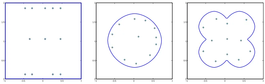
• Three domains; a square domain Ωs, a circular domain Ωc ⊂ Ωs and a quatrefoil domain Ωq⊂Ωs, see Figure 1. For the curved domains Ωcand Ωq we used numerical integration to approximateskl,k, l= 1, . . . , L.

• The set K is chosen in the following way. We choose the φi, i = 1, . . . , L to be

the basis functions associated with vertices of triangles belonging to a uniform right angled isosceles triangulation of Ωsformed on a square grid of size (J+ 1)×(J+ 1), with triangles of diameterha. We set Am = 0.1 andAM = 5.

The observed data are generated as the exact arrival times on the boundary arising from given slowness functions. We use the three values of the slowness functiona= 1/c consid-ered in [11]:

c(x)≡1; (4.8)

−10 −0.5 0 0.5 1 0.5

1 1.5 2

−1 −0.5 0 0.5 1

0 0.5 1 1.5 2

−10 −0.5 0 0.5 1

0.5 1 1.5 2

Figure 1: The distribution of 12 source points in Ωs_h (left hand plot), Ωc_h (centre plot) and Ωq_h (right hand plot)

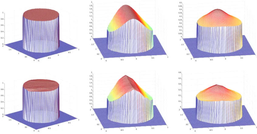
In Figures 2–4 we show several examples of the recovered and exact slowness functions. They were obtained with h= 0.02. In Figure 2 we take Ω = Ωs,L= 121, J = 10, δh =h

and S= 12 (see Figure 1 for the distribution of the source points). The upper plots show a(x) given by: (4.8) left hand plot, (4.9) centre plot, (4.10) right hand plot, and the three lower plots show the corresponding approximate solutionsah(x). Figures 3 and 4 take the

same form as Figure 2 but with Ω = Ωc, L = 65 and J = 10 and Ω = Ωq, L = 75 and J = 10 respectively.

S a(x) given by (4.8) a(x) given by (4.9) a(x) given by (4.10)

1 7.64·10−5 (3.45·10−2) 3.90·10−2 (5.46·10−1) 3.16·10−4 (5.65·10−2) 5 4.26·10−6 (2.17·10−3) 6.52·10−2 (1.87·10−1) 8.26·10−4 (1.94·10−2) 9 2.19·10−6 (1.43·10−3) 6.79·10−2 (1.61·10−1) 8.68·10−4 (1.67·10−2) 12 2.22·10−6 (1.30·10−3) 7.83·10−2 (4.80·10−2) 1.00·10−3 (5.61·10−3)

Table 1: J_h(ah) (ka−ahk0) for Ωsh,L= 121, δh =h

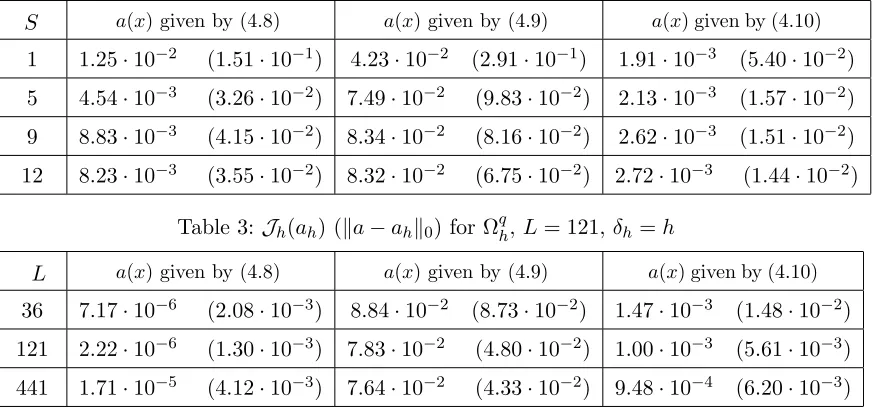
In order to get some idea of how the parameters in the model affect the solution we include Tables 1–6. In these tables the values of J_h(ah) = minKJh and ka−ahk0 are displayed.

Unless otherwise specified the data in Tables 1–6 were obtained by setting Ω = Ωs,L= 121, δh =h and S= 12.

• In Tables 1-3 for each of the slowness functions defined above we consider four values for the number of source pointsS.

• In Table 4 we consider three values ofL.

Figure 2: a(x) (upper plots),ah(x) withL= 121,δh=h and S = 12 (lower plots)

Figure 4: a(x) (upper plots),ah(x) withL= 121,δh=h and S = 12 (lower plots)

S a(x) given by (4.8) a(x) given by (4.9) a(x) given by (4.10)

1 3.33·10−5 (1.20·10−2) 1.80·10−2 (2.25·10−1) 2.32·10−4 (4.08·10−2) 5 1.12·10−4 (7.16·10−3) 4.10·10−2 (3.15·10−2) 8.63·10−4 (5.16·10−3) 9 3.21·10−5 (9.40·10−3) 4.59·10−2 (2.66·10−2) 9.99·10−4 (4.00·10−3) 12 3.40·10−5 (8.40·10−3) 4.70·10−2 (2.68·10−2) 1.01·10−3 (4.15·10−3)

Table 2: Jh(ah) (ka−ahk0) for Ωc_h,L= 121, δh =h

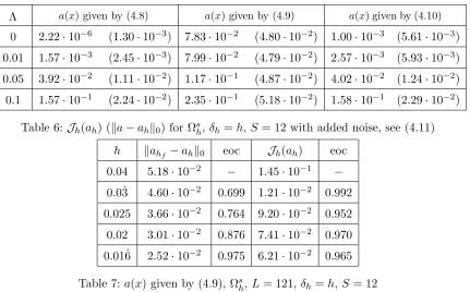
• In Table 6 we add noise into the system; in particular for each of the desired speed functions, (4.8)–(4.10), we solve (2.4) to obtain ˆu(xα) and then we set

uobs(xα) = ˆu(xα) + Λn(xα), xα∈Gh (4.11)

wheren(xα)∈[−1,1] is random noise and Λ∈R.

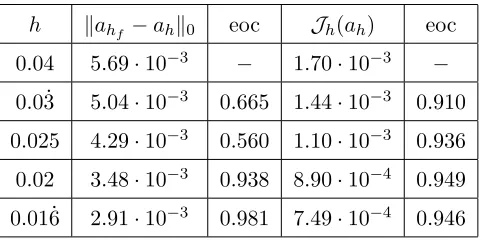
We conclude our numerical results with Tables 7 and 8 which show how kahf −ahk0 and

J_h(ah) = minKJh vary with h. Here we fix the convex set K by setting L = 121. The

S a(x) given by (4.8) a(x) given by (4.9) a(x) given by (4.10)

1 1.25·10−2 (1.51·10−1) 4.23·10−2 (2.91·10−1) 1.91·10−3 (5.40·10−2) 5 4.54·10−3 (3.26·10−2) 7.49·10−2 (9.83·10−2) 2.13·10−3 (1.57·10−2) 9 8.83·10−3 (4.15·10−2) 8.34·10−2 (8.16·10−2) 2.62·10−3 (1.51·10−2) 12 8.23·10−3 _(3.55·10−2_{) 8.32·10}−2 _(6.75·10−2_{) 2.72·10}−3 _(1.44·10−2₎

Table 3: J_h(ah) (ka−ahk0) for Ωqh,L= 121, δh =h

L a(x) given by (4.8) a(x) given by (4.9) a(x) given by (4.10)

36 7.17·10−6 (2.08·10−3) 8.84·10−2 (8.73·10−2) 1.47·10−3 (1.48·10−2) 121 2.22·10−6 (1.30·10−3) 7.83·10−2 (4.80·10−2) 1.00·10−3 (5.61·10−3) 441 1.71·10−5 (4.12·10−3) 7.64·10−2 (4.33·10−2) 9.48·10−4 (6.20·10−3)

Table 4:Jh(ah) (ka−ahk0) for Ωs_h,δh =h and S= 12

computed on a fine grid withh= 0.005 andah is the approximate solution computed using

h = 0.05,0.04,0.0 ˙3,0.025,0.02,0.01 ˙6. From these tables we see that for the two desired speed functions, (4.9) and (4.10), the values ofkahf −ahk0 and Jh(ah) = minKJh reduce linearly with h.

References

[1] R. Abgrall. Numerical discretitzation of boundary conditions for first order Hamilton– Jacobi equations. SIAM J. Numer. Anal., 41:2233–2261, 2003.

[2] R. Abgrall and J. D. Benamou. Big ray tracing and eikonal solver on unstructured grids: Application to the computation of a multi-valued travel-time field. Geophysics, 64:230–239, 1999.

δ a(x) given by (4.8) a(x) given by (4.9) a(x) given by (4.10)

0 2.62·10−5 (1.61·10−2) 1.07·10−4 (2.84·10−2) 9.75·10−6 (6.07·10−3) h2 2.92·10−5 (1.45·10−2) 1.74·10−2 (2.42·10−2) 3.14·10−5 (5.91·10−3) h 2.22·10−6 (1.30·10−3) 7.83·10−2 (4.80·10−2) 1.00·10−3 (5.61·10−3)

Λ a(x) given by (4.8) a(x) given by (4.9) a(x) given by (4.10)

0 2.22·10−6 (1.30·10−3) 7.83·10−2 (4.80·10−2) 1.00·10−3 (5.61·10−3) 0.01 1.57·10−3 (2.45·10−3) 7.99·10−2 (4.79·10−2) 2.57·10−3 (5.93·10−3) 0.05 3.92·10−2 (1.11·10−2) 1.17·10−1 (4.87·10−2) 4.02·10−2 (1.24·10−2) 0.1 1.57·10−1 _(2.24·10−2_{) 2.35·10}−1 _(5.18·10−2_{) 1.58·10}−1 _(2.29·10−2₎

Table 6:J_h(ah) (ka−ahk0) for Ωsh,δh=h,S= 12 with added noise, see (4.11)

h kahf −ahk0 eoc Jh(ah) eoc 0.04 5.18·10−2 − 1.45·10−1 −

0.0 ˙3 4.60·10−2 0.699 1.21·10−2 0.992 0.025 3.66·10−2 0.764 9.20·10−2 0.952 0.02 3.01·10−2 0.876 7.41·10−2 0.970 0.01 ˙6 2.52·10−2 0.975 6.21·10−2 0.965

Table 7:a(x) given by (4.9), Ωs_h,L= 121, δh =h,S= 12

[3] M. Bardi and I. Capuzzo-Dolcetta. Optimal control and viscosity solutions of Hamilton-Jacobi-Bellman equations. Modern Birkh¨auser Classics. Birkh¨auser, Boston Basel Berlin, 2008.

[4] J. D. Benamou. Big ray tracing: Multivalued travel time field computations using viscosity solutions of the eikonal equation. J. Comp. Phys., 128:463–474, 1996.

[5] J. M. Berg and N. Zhou. Shape-based optimal estimation and design of curve evolution processes with application to plasma etching. IEEE Trans. Auto. Control, 46:1862– 1873, 2001.

[6] J. G. Berryman. Stable iterative reconstruction algorithm for nonlinear traveltime tomography. Inverse Problems, 6:21–42, 1990.

[7] I. Capuzzo-Dolcetta and P. L. Lions. Hamilton–Jacobi equations with state con-straints. Trans. Amer. Math. Soc., 318:643–683, 1990.

h kahf −ahk0 eoc Jh(ah) eoc 0.04 5.69·10−3 − 1.70·10−3 −

0.0 ˙3 5.04·10−3 0.665 1.44·10−3 0.910 0.025 4.29·10−3 0.560 1.10·10−3 0.936 0.02 3.48·10−3 0.938 8.90·10−4 0.949 0.01 ˙6 2.91·10−3 0.981 7.49·10−4 0.946

Table 8:a(x) given by (4.10), Ωs_h,L= 121, δh =h,S= 12

[9] K. Deckelnick, C. M. Elliott and V. M. Styles. Optimal control of the propagation of a graph in inhomogeneous media. SIAM Journal on Control and Optimization, 48:1335–1352, 2009.

[10] H. Ishii. A simple, direct proof of uniqueness for solutions of the Hamilton–Jacobi equations of eikonal type. Proc. Amer. Math. Soc., 100:247–251, 1987.

[11] S. Leung and J. Qian. An adjoint state method for three-dimensional transmission traveltime tomography using first-arrivals. Commun. Math. Sci., 4:249–266, 2006.

[12] P. L. Lions. Generalized solutions of Hamilton-Jacobi equations. Pitman Advanced Publishing Program, 1982.

[13] A. Sei and W. W. Symes. Gradient calculation of the traveltime cost function without ray tracing. In 65th Ann. Internat. Mtg., Soc. Expl. Geophys., Expanded Abstracts

1351-1354 Soc. Expl. Geophys., Tulsa, OK, 1994.

[14] J. A. Sethian. A fast marching level set method for monotonically advancing fronts.

Proc. Nat. Acad. Sci. U.S.A., 93:1591–1595, 1996.

[15] J. A. Sethian. Level set methods and fast marching methods. Volume 3 ofCambridge Monographs on Applied and Computational Mathematics. Cambridge University Press, 1999.

[16] H. M. Soner. Optimal control with state-space constraint. SIAM Journal on Control and Optimization, 24:552–561, 1986.

[18] C. Taillandier, M. Noble, H. Calandra, H. Chauris and P. Podvin. 3-d refraction traveltime tomography algorithm based on adjoint state techniques. In 70th EAGE Conference and Technical Exhibition, Eur. Ass. of Geoscientists and Engineers, Rome, Italy, 2008.