The application of multivariable optimal control to non linear chemical processes

MULTIVARIABLE OPTIMAL CONTROL

TO

NON-LINEAR CHEMICAL PROCESSES

A THESIS SUBMITTED FOR THE

DEGREE OF

DOCTOR OF PHILOSOPHY

IN

CHEMICAL ENGINEERING

IN THE

UNIVERSITY OF CANTERBURY

CHRISTCHURCH, NEW ZEALAND,

BY

ToP. DOBBIE

_:;:/

My greatest thanks are due to Professor A.M. Kennedy for his very considerable support throughout the long course of this study. His unobtrusive encouragement and his abIlity to find financial assistance, through the University of Canterbury. were greatly appreciated. 1 would also like to acknowledge financial assIstance from the Fletcher Holdings' Postgraduate Scholarship In Chemical Engineering.

I am also indebted to my triend and supervisor Dr W.B. Earl tor assistance and advice. The project may perhaps have proceeded faster had Brian been less of a friend and more of a supervisor, but I would prefer it no other way.

1 extend my sincere thanks to all the staff of the Chemical Engineering Department and to my fellow post graduate stUdents tor their friendship, interest and stimulating discussion over the .past tew years. In partIcular 1 .ould like to acknowledge the generous assistance ot of Mr P.J. Jordan which was greatly appreciated.

For providing the opportunity to start this course ot study, tor the very real sacrifices she has made throughout its duration and for her consideraole aSSistance in seeing the project throuyh to a satIsfactory conclusion I must thank my wife Gay.

CONTENTS

ABSTRACT

CHAPTER

I

INTRODUCTION

II

MODERN CONTROl. TECHNIQUES

III

DYNAMIC PROGRAMMING

IV

FEEDFORWARD CONTROL TECHNIQUES

V

OPTIMAL FEEDBACK CONTROL OF LINEAR

SYSTEMS

VI

CONTROL OF NON-LINEAR STIRRED-TANK

REACTORS

VII

EXOTHERMIC

NON~LINEAR

REACTORS

VIII

DISCUSSION AND CONCLUSIONS

REFERENCES

APPENDIX

I

CONTINUOUS SYSTEMS MODELLING PROGRAM

II

SYSTEMS SUBROUTINES FOR MULTIVARIABLE

OPTIMAL CONTROL

PAGE

1

3

17

33

49

59

83

103

127

136

140

Higher production rates, more extreme processing conditions, tighter product specifications and more highly integrated processing plant are envisaged as some of the reasons

for encouraging the chemical industries to look more closely at the potential advantages of Modern Control Techniques. The advent of the proce~s control computer has failed to bring about any significant shift away from the established conventional control techniques, perhaps because of the innate conservatism Of the control enqineers but more likely due to the apparent complexity of the mathematical techniques

control, and a lack of confidence

involved in so-called "Optimal" in the ability of optimal controllers to perform significantly ~etter than the already

highly~developed slngle~loop controllers.

The aims of tnis study are tWo=fold:

(1) To demonstrate straightforward techniques for the solution of the optimisation problems which are the basis of optimal control theory, and

(2) To demonstrate, by lmplementation of the control laws so obtained, ~ome. of the advantages Which can accrue from multi variable optimal control.

Some

introduced

development technique.

The control laws are tested an a range of linear and non-linear systems and their performance compared With that of single-and multi-loop controllers under conditions ot bounded controls, random disturbances and process and control variable "dead-time". The particular advantages of multivariable controllers are found to be

(1) More effective control, as measured by the process control criterion,

(2 ) An ability to stabilise the process under more severe disturbances,

(3) Greater procels stability In the face ot process or control variable "dead-time",

(4) The use of significantlY less control effort in controlling the process, and

(5 ) 1'he ability to control naturally unstable processes with tiqhter limits on the control variables.

Multivariable feedforward controllers are also developed and are shown to have significant advantages even on single-stage processes, although the quality of the process model Is shown to be important. A non-linear feedforward compensator Is seen to possess quite dramatic load rejection potential.

The mUltivariable optimal controllers are thus seen to be reasonably Simple to implement, robust In operation and very effective. Possibly the greatest single advantage of mUltlvariable over multi-loop control strategies is the elimination, at a stroke, Of the confiquration problem •

CHAPTER I

INTRODUCTION

"Between the idea and the reality falls

shadow •••

11

T.S. Eliot

The current status of Control Science is reviewed in

ion to the Chemical Processing Industries and the spl

between the established control practices and the modern

control theories is analysed.

L l

1.2

1.3

1 4

1.5

1.6

1.7

1.8

Introduc

Single-Loop

Multivariable Control

Convent

Multi~Loop

Technology

Automat

Measurement

Analytical

Techniques

Process Control Computers

Chemical Process Plant

Modern Control Theory

Comparison of Multivariable and Multi-Loop

Control Strategies

Page

4

7

8

10

1'1

12

12

13

INTRODUCTION

One of the first examples of the application

cif

automatic control was the centrifugal governor designed by James Watt to control the speed of a

steam engine. No longer did an operator have to concentrate slavishly on the machine's speed to control th~ steam pressure with a hand valve, and neither did the machine's performance depend so entirely upon the concentration, skill or whim Of the human link in the feedback chain. Considerable progress has been made In all aress of automatic control over the Intervening two hundred years If we consider tne huge modern processing cDmplexes controlled automatIcally under the almost casual supervision of a few men. The progress of control SCience has by no means been steady.

however, and neither, as we shall see, has there been unanimity withIn the ranks of control engineers as to the best means of achieving its objectives. Thp mathematIcs and application of OPtimisation and automatic control

received a boost during the latter years of the second wDrld war, much of

which did not see the light of day. New theories were taking shape however, and once their 1 rest had been kindled, people took their experience and skills into other areal In more recent time • but in muCh

the same way, the Hsp!n offs· from the aerospace indu try have re ulted in a

flood of new technologies.

The post-war years saw a steadily increasing interest in control

theory and practice, particularly the systematic development of the Calculus of

came

Va lations

in the

as a technique for process optimisation. The greatest boost late 1950's and early 1960's largely beCBuse of two developments. These were the very rapid advances being made In computing equipment and techniques, and the consolidation of var! ional methods

-loosely known as Modern Control Theory. 1962 saw one of the landmarks in control theory and application with the first publication in English of the pioneering work of Pontryagln, Boltyanskil, Gamkrelldze and Mishchenko, "The Mathematical Theory of Optimal processssp

• With Bellman"s works. "Adaptive

Control Processes" and "Applied Dynamic ProgrBmm n the future of Modern Control Theory was Bssured. A flood of books

.nd

papers was to folloW, but

(1967), Noton (1965) and the most wIdely referenced book of all by Athens and Falb (1966).

Within the chemical industry developments were steadily changing the nature of chemical plant and, ind@ed~ the processes themselves. Spurring these developments along was the rapid growth in the output of chemical

industry and in the diversity of its products, with the consequent increase

in new proceSSing installations. Plants were increaSing in size and

throughPut with each new generation bringing a huge increase In productivity. The economies of scale gave considerable impetus to the

installation and improvement of process control equipment. Batch plant was

giving way to continuous processes, espeCiallY where Increased demand

virtually excluded the possibility of economic batch processing. With the

shift to continuous processes came the trend toward more integrated plant.

No longer were individual plant items independent of each other, with large storage vessels acting as buffers to isolate them from upstream or

dOWnstream emergenCies. Processes became more complex, with several "unit

operations" sometimes incorporated into a single piece of equipment. A

factor related to the change toward m6re integrated plant was the increase

in processing "rate". Older plant was being pushed to its maximum capacity

(and beyond) and new plant deSigned to increase throughPut with the minimum

physical plant size. Residence times became shorter and processing

conditions more extreme, and the performance of control systems rose to meet

the demands.

A graphic comparison may be found in the production of Sulphuric

Acid~ long used as an index to the growth of the chemical industry. The vast "Lead-chimber"-Plants with reildence times 6f ~any hours could cover a

hectare of land to produce a hundred tonne per day

Of

70% acid. "Contact" plants had taken over almost entirely by the 1960's, 300 tpd plants occupied no more than 1000 square

metres

and produced 98% ~cid and large quantities of process steam. By the 1970·& a plant of dOUble ,the capacity occupied a site half the size or smaller with faster reaction rates, shorter residence times and higher operating temperatures and pressures.

Eliminating the storage of

overall size of the plant but each

intermediate products decreased

unit now fed its product and

the

disturbances dIrectly into th~ unit downstream An undetected or uncorrected disturbance could affect 8 whole section of plant to the detriment of product quaIl and operating economics. Improvements in the control of the ~rocesslng

environment

may prevent some of the disturbances

from

reaching vital or unstable plant, or at least reduce the damaging ffeets, but many chemical processes femain very susceptible to product variability which cannet be entirely eliminated. Because of this the chemical manufacturer 'must frequ~ntlY aim at a product specification exceeding that required by the purchaser, with consequent increase In costs or decrease In prodUction rate, just to enlure that the natural variability o the process doe not result In an unlBleable product.

Increased competition In the chemical market place led also to the general tiqhtenlng of chemical and Physical specifications encouraging

19hter control of the manufacturing processes.

Recently two new factors have emerged which are having a very major influenc on the chemical proces Ing industri The rapidly Increaslnq cst and r it ieted upply of most forms of energy and closely related, the ncr sing cost 0 petroleum. the baSic fee tack or a considerable

propor ion of the chemical indus

Throughout the 1 t two decades the ncentlve& for improvement In all peets of process control could hardly have been greater the same two decades which saw the most dramatic developments In the establishment of Modern Control Theory HOW, then, was it possible for the new control theories and the established control practices to continue to develop and apparently thrive

In virtual

·~f each other~s existence?

relation to the other to understand how this may have come aboutQ And to do

that it Is important to distinguish clearly between the modern control theories and th~ conventional approach to control system sYnthesis •

••••• DOODOOOaOOD •••• ~

1.1 SINGLE~LOOP CONTROL

The science of contral grew from the single-Input, single-output

analysis of systems. Early "unit operations" equipment was generally

operated at the level of sophistication which recognised a one-to-one relationship between the process variabl@s and early Automatic controllers implemented this philosophy. The process operator, as he learnt the

idiosyncrasies of his pl~nt. recognised the interaction effects and, if sufficiently killed, used them tD good effect. As interaction ~f ects became more readily Identified and quantified some wer exploited in cascade

controllers, but the basic prlnclpl of single-loop controllers remained.

Even with the introduction of very obviously multi-input, multi-output

processes and a greater understanding 0 the chewical and physical

relationships involved the control systems remained essentially a collection

of single-loop strategies

One of the reasons

la~l translei function for

dominated the mathematical

for this must surely be the adherence to the

analysis whicfi has ri~til recently

treatment of automatic control. Although both

laplace domain and frequency domain techniques are adaptable to multi-input,

mUlti-output systems there!s something inharently clumsy about matrices of

transfer functions. There l~ af course a direct correspondence between

laplace and linear state-space presentation and all the operations in one

domain have direct counterparts In the other.

In Single-loop control each control variable

deViations of only one procell variable. The deViations

Is governed by the

would be beneficial in festoring those other variables to their respective

set points. Neither Bre the interaction effects between the control

variable and the other. variables consIdered, exce~t of course In the controller tuning once the plant lsopefating.

The control system·. engineers were probably not chemical engineers

and did not fully understand the chemical and Physical phenomena they were attempting to control. It BeemB certain that the process designers did not

set out to model the procell with algebraic and dynamic equations for had

they done 50 they could have hardly helped but notice the fundamental

interactions between variables whIch are so obvious from the state-space

representatlon&

OOODDODDOOO •••• ~

1. ~ULTI-VARIABLE CONTROL

Mu tlvarlable control recogni ~ and u the dynamic and alqebraic

relationships between variable. Each control variable 1 a function of all

the process variables over which it has an influence. When any or all of the proce s variables deViate from their set-points the influence of the

control variables on the system 15 to force the return of each variable to

it s~t-p~lnt

it

a rate which re

to

pe~alty ~laced upon its

deviation.

that

This raises another .essential feature of Modern Control

Is the ext tence of a Process Control Criterion.

Theory~ and

The process

controller 1s deSigned to optimise a process control criterion however

arbitrary that may appear to be, and involved 1n the choice ot that

criterion is the priority attached to the actions and interactions of the

process Variables. With the well-established Quadratic Error criterion,

such that the algorithm which optimises thl control criterion is directed to reduce most rapl y the deviations of the most heavily penalised variables.

In a compact integrated plant the interactions between variables

raises another major problem for singleoloop control strategies that of

configuration. With SO many alternatives to choose from haw does the

,

control engineer choose the best feed-back loops for process stabl11satfon?

In a hypothetical, exothermic reactor does he use the deviation of the

product concentration to control the feed rate, the supply of catalyst, th~

level of reactants in the reactor or the flow of coolant? Although

intuition and Modern Control Theory say "use them all]" the conventional control engineer must decide on just one, and make similar, perhaps arbitrary, decisions for the other loops as well. Cascadinq of control

loops and the use of decoupling algorithms may go some way toward improvinq

the quality of control. but tne problems of the control engineer are only

compounded by the Increasing number and complexity of the possible

candidates for the control loop configuration.

The dependence of the control variables on all the state variables

means that a dynamic optimisation can be ffected by the control function

instead of the tatic optlml at10n per med by a sinqle loop cont 01

strategy. Returning to the exothermic reactor example; a change In feed

concentration may be compensated mOlt rapidly and economically by adjusting

the reactor temperature. If, however, the coolant flow-rate 15 controlled

only by the reactor temperature thIs dynamic compensation cannot be

employed. The

reactor temperature

will eventually fluctUate because

of

the effect of the changed feed concentration on the reaction ratev but the

response of the temperature controller will be delayed and the effect will

be to try to restore the reactor temperature to the original set-point and

not the temperature relevant to the current feed con~entratlon. In effect, the action of the tempera~ure controller will be contrary to the objective of maintaining a steady product concentration. Borer(1974) details the

importance of dynamic compensation and emphasises the point (1977) with the

comment that;

conversion ratel, etc. tnen control must Increasingly be exercised on a dynamic basis. Single loop regulation of individual process parameters is no longer adequate; disturbances cannot always be

subdued before they enter the process and must absorbed by

permitting certain variables to change transientlY In a controlled fashion."

If only lome of the apparent advantages of multlvariable control are able to be realised on a chemical plant it Is still somewhat surprising to find such an obvious gap between the theory and the practice of modern control techniques If, as is confidently predicted, process stability

could be enhanced and product variability decreased by the use of multivarlable controllers then Why are control engineers and plant managers still wedded to the conventional control technology? The reasons are as

nUlnerous and as dIverse as the Chemical industry itself but a brief analysis of a tew would be in order.

• •• 00000000000

.0.

1 3 CONVENTIONAL MULTI-LOOP TECHNOLOGY

"Better the devil you know

The chanqes in chemical industry and the demands of new technoloQY have, i n r a l . been ly met by Improvements in conventional control. Operating speed and preciSion have increased and Where necessary the slower and mor~ cumbersome pneumatic systems have been supplanted by

Above all thiS 1& the accumulation of experience which, for example,

makes the configuration problem relatively tractablec

1.4 AUTOMATIC MEASUREMENT AND ANALYTICAL TECHNIQUE&

Improvements In measurement technology have qreatly assisted the

control engineers In keeping up with modern processes, particularly the wide

range of on-line automatic analysers. In the area of chemical analysis the

range of automated techniques is extensive. Continuous monitoring of ionic

concentration by specific ion electrodes is common, as 15 the discrete

analysis by automatic titration. UltraViolet and infrared spectrophotometry

are alSO readily used on- ne as are the very widely used chromatographic

techniques. Even solids can be utomati 11y analys d by methods uch as

ray dl fraction and fluorescence There are many technique available for

the on-line measurement of physical pa amet density, visco ity,

refractive index, temperature, colour, turbidity, flow-rat, and

conductivity may be IV determined for gases, liquids, and solids ranging from powde s to larger particulates. The accuracy and speed ot

these analytical techniques are being stead! improved and many of the

currently regarded off line techniques may 500n b@ fully automated fo

greater assistance with process optimisation and control •

1.5 PROCESS CONTROL COMPUTERS

The intro~uctiDn of digital cDmputers to the chemical Industry

brought cons!derabl advances to the science of control. As the digital

computer i5 essentially a sampled-date machine it b~ought about something of

a revolution In data acqUisition and transmisSion, procell representation

and modelling, and the design of control algorithms. The speed of the

digital computer meant that a much wider range of activities could be

accommodated, including complex multi-looP control strategies and on-line

optlrllisation.

• •••• QOOOOOOOOOO •••• ~

1.6 CHEMIC~L PROCESS PLANT

I f the .1 one factor which characte is B chemical processes it

would surely b non-lineari

Non-Llnearities abound In systems involved with heat, mass and

momentum transf r, thermodynamics, reaction and catalysis and all the staged

and recycle processes which render anal leal techniques unworkable. Two

other effects. endemiC to chemical plant and similarly confounding the

analytical approach, are hard ~onstrBlnts on ~rocesl and control variables,

and time delays.

Local 11nearisation. Is usually posBible but the non-linearlties may be so extreme that the region over which the lineari$atlon may be applied Is

very :;mall

1.7 MODERN CON'l'ROL 'tHEORY

,.

_o Q Q than the davil you don to"

Modern control theory 1 unfortunately obscured and misrepresented by

writers luch as B (1973) In hi "critique" of chemical process control theory and luch reactionary attitude are unfortunate. certainly the problems associated with the design and application of Modern Control techniques are very far rom any general solution, however the theoretiCians have furnished U5 with a set of elegant theories, complete with necessary

Bnd sufficient eonditlDns for global optimality In contradiction to Foss, therefore, the ball Is no longer In the theoreticians' court but very firmly established in the court of the control engineer.

For example: Local I1nearisatlon and judicious application of the

quadratic error criterion result In a system for whiCh's general solution

has been established That a model of the nece sary 1 not too great 8 hardship.

process to

I f the proce

be controlled is

1

stages (surely the bes ime to be Signing the control system) a

mathematical model a 1 mandatory fo good sIgn the

proce 5 is

b~~netit in

appropriate

a modelling exerc could be gr t unde tanding the p IS. and If an analytt 1 approach is not

then Identl 1catlon techntque could b employed. Bard

constra nts? ti and acute ~on Inearltles B occasionally the

result of poor design and a such may be revealed by a detailed analysis of

the process. The cost of replae a large diameter pipe with a small one

and Inst 111nq a pump to overcome the increased pres sur drop or replacinq

a control valve wit~ one l~rger or faster. might be recovered in a matter of weeks by the reduced product Variability due to faster and more positive control action.

model reduction techniques are available which will specifically retain the

particUlar process dynamics that are regarded as Important. SimilarlY the

problem of lnacelBlble states may be accomodated by judicious model

reduction or by the techniques af state and parameter tlmatlon.

For the simplest case o~ time-invariant p.rRm~ters and Infinite

horizon the implementation of ~ multlvorlable controller requires less control hardware than the ~quivalent multioloop system with & separate controller for every loop_ Workable algorithms are available from most

modern texts on the subject of process control and could be applIed by most

engineers with a reasonable know of linear algebra. Even discounting

the analytical approach Which Is pOSSible, if tedious, for systems ot low

order, the algorithms are readily programmed and solved off line by a very

mode t computer. Contrary to popular belIef a diqital computer is not essential for the implementation of a multi-variable controller, although

the existence of an on~llne computer eould improve the quality of control by means of non$llnear controllers or with the techniques of state estimation,

parameter tracking and proees optlmllatlon~ The ule of Modern Control techniques would require no more technical expertise than conventional

control strategies

1&8 COMPARISON OF MULTIVARIABLE AND MULTI-LOOP CONTROL STRATEGIES.

Managers of chemical process plant. along with their process

designers and control systems engineers, ar~ essentially bUSinessmen - hard~

headed and a bit conservative, and therefore unlikelY to abandon

tried and proven methods unless a new system can prove its superiority in

terms of processIng economicse The stage has long since been reached In the

Conventional control technology has continued to survive under the

condltlons imposed hy chemical processing; Imprecise models, drifting

para~eters. measurement error. hard constraints and unavoidable dead-times. Unless the application of Modern Control Theory can consistently out~perform

tn.

established conventional control techniques the holders of the chemical

industrie • purse strings will continue to ignore it. And who could blame thpm?

MODERN CONTROL TECHNIQUES

The State Variable form of process representation

is introduced and some of the modern techniques for control

system synthesis are examined.

Page

2.1

State Representation of Dynamic Systems

18

2.2

Discrete~time

State Equations

20

2.3

Eigenvalues and the System Response

21

2.4

Controllability and Observability

23

2.5

The Development of

Single~Loop

Control Laws

24

2.6

Modern Control Techniques

25

2.7

Direct Search Techniques

26

2.8

Modal Control

27

2.9

Variational Methods of Optimisation

29

2.10

The Calculus of Variations

29

CHAPTER II

MODERN CONTROL TECHNIQUES

2.1 STATE REPRES~NTATION OF DYNAMIC SYSTEMS.

In the development and discus.lon of various

construetinq mUltlvarlable control algorithms the dynamic

represented exclusively In State Variable form. The

conversion between 11n~ar state variable and laplace

summarised by Ward and Strum (1970) and Noton (1972). The

techniques for

systems will be

techniques for

torms are we 11 development of

mathematical models ot chemical processes In state variable form is covered

In many modern texts and the apPlication to particular ~ystems will be described in some detail 1n l~ter chapters. The most general form of state variable representation of a process is

• • • • • (2 1)

1

=

I, 2, ~ ••• n where x 1 the state vector, ~ is

vector of disturbance varlabl

vector of control variables and d is a

Where the process Is linear, or may

reasonably be 11nearlsed about a point In tate space. the pr p esented In the standard non-homogeneous linear form

55 may be

x A(t) ( t ) t B(t)u(t) + C(t)d(t)

where A 1 the state matrix and 8 and C are driving matrices relatinq to the control inputs, Up and the procesl dl lurhance inputs, d. respectively. The

driving matrices are sometimes combined into a lingle matriX and a combined

vector i& formed from the control and disturbance vectors ThiS 15 the most

compact linear form but

between those inputs

it t~nds to obscure the important distinction

which may be manipulated to optimise the process and

the uncontrolled disturbance, or "load", variables.

Despite the dexter ty with which analogue and digital computers can generate solutions (or trajectories) for sets of non-linear diffprential

equations there are considerable advantages in the use o£ linear equations

For non-linear systems the effort involved In determining truly optimal control algorithms is very considerable and generally prohibitive for on Une work. Conversly, local linearisatlon and the development and apPlication of linear controllers is generally more straightforward and should appeal to engineering pragmatism.

For a process modelled by a set of non-linear equations

x

~ f(X,U,t)

it Is possible to linearis8 about a pOint

(X,D),

or perhaps a nominal trajectory (X(t),U(t)), by defining deviation variables x, u such that

u

The model may be expressed In terms of these new

variables

=

f(x,u,X,U,t)

•••••• (2.4)

and may then be Ilnearised about a point or nominal trajectory, by

calculating the Jacobian matrices J. and J_u whose elements are given by

and

af

_~J

••••• (2.5)

and are evaluated at the point or along the trajectory about which the model was to be linearlsed The Jacobean matrices J_{x and} J_u are the state and driving matrices respectively.

The general solu Ion to sets of linea equations of the form

=

A(t)x(t) + B(t)u(t) 0 • • (2 6}

may be expressed as

x(t)

-t

<l> (t • to lx (to) ,

J

<l> ( t • t ) B (t ) u (1 ) d1

to

• • •• • (2 .,)

where $(t,t

_{o )}

Is known as the TranSition matrix and 15 defined as the solution to the homogeneous matrix differential equation

d

dt

¢ (

t , to)::: A ( t )

¢

(t, to ) • • • • • (2.8)

for all t. The solution to this equation for a time. invariant 5tBt~ matrix A takes the form of a matrix exponential

¢(t,t

_o)

=

eXP(A(tet

_o

»)

which may be expressed ana evaluated as the matrix series

exp(A(t~to) :: I + A(t~to) ... A 2( te _t

o ) 121 ...

and Which can be ahown to converge ablot and uniformly on any finite interval of the time axis, (TOd. 1964), and Is readily programmed for

solution by digital computer (Notan. 1972, Kalman and Englar, 1966, Melsa, (970). The proof of the existence and un

lolution for the general calev and its non-s

IS of the matrix Ie les

larlty for all (t,t_{o )'} Is

given by Bellman (1967). There are problems with truncation and rate of

convergence however when the matrix A(t ) Is large and the time interval

(t"'t_{o ) may have} to be fl!':duced 1n order to effect a satisfactory numerical

solution. The solution to the part woUld generally be

calculated at the same time provided the charac lstlcs of the forcing

fUnction, u

comprising the sum

known over the range (t, ). The complete solution,

the free and forced responses, may be expressed in terms of the tran Itlon and driving matrices

x(t)

• • • • DDOOOOOoooo •••• ~

2b2 DISCRETE-TIME STATE EQUAT DNS

The application of iglt&l computers to process control requir the

development of diserete~tlme models. The digital control computer a

5Bmpled~data device and the computations are handled In a stage-Wise fashion. A process model must therefore be devised to provide information on the state variable trajectory at discrete Instants corresponding to the

control computer"s view of the continuous process This Is done by solvinq

the set of continuous differential equations over the discrete time Interval

T assuming piecewise continuous

The solution. once again str

for the duration of the interval

orward for sets of linear equations,

involves the evaluation of the transition and driving matrices

¢>( t" to) :;;::

L\(tpt

_{o )}

~

expressed as the sum of a transformation of the state at the previous

sampling instant and the eff~ct of the process inputs for the duration of that stag~, loe.

)«(I<+1)T)

=

VCkT)xCkT) + ~(kT)u(kT)

This may be expressed more conveniently as

X(k+l)

=

~(k)K(K) ~ 6(k)U(k)

interval Is implied, or even

Xk+1 ~kl(l<+ ~kUk

. e o • • (2.13)

where the sampling

The more compact subscripted form of aquation 2.14 is preferred where

it Is clear from the context that the subscript refers to the stage and not to a specific element In th@ vector

9~'. 00000000000 19 G e.o

2.3 IGENVALUES AND THE SYSTEM RESPONSE

The choice 0 the s~ate variables 1 generally traightforward for chemical proceSSing systems, uslnq either basic 0 derived measurements.

The state 0 sucrose solution 1n an evaporator might be desc ibed in te ms

of Temperature and Concentration but for the purposes of on line analysis

the state may be more conveniently measured In terms of its density and

refractive index. Temperature and concentration are however independent

modes in that either may change (within limits) wi hout affecting the other,

whereas a change In density, for eXample, brought about by a chanqe In either temperature or concentration, would also have an effect on the

refractive index. There are a number of physico-chemical properties of the

sucrose solution which could be measured, indicating that the choice of

state variables Is not unique, but there i one set of state variable , the

dynamic behaviour of which dlsp the system structure In its most basic

form because of their lack of interaction with one another. modes are

linear combinations of the measured properties and are known as

eigenvectors, and the transformation of the states into the respective

For a lInear dynamic process

.

x

let . th~ linear trans ormation Which achieves this decoupl1ng of the state variables be P, such that

then p-1

X

p-l (APz + fill)

:= p-1 APz + p-1 Bu

and the state matrix which maKes the transformed state variables independent is the dlaqonal matrIx of eigenvalues. or Spectral Matrix,

•••••• Ci!.16)

The free time-response of the modes 1&

and the mode will be stable If the real part of the eigenvalue ~i' is negative. For complex eigenvalues the system response will be oscillatory.

For dl rete time systems the reapon! 1s given by

(2.lB)

and the proces is tabl i the sequence of euclidean no ms

vector

Ilx(k)!I

Is decreaslnq monotonic sequenc~.

For thiS to be 50 the necessary and su flcient condition Is 11<1>11 < 100 implying that the eigenvalues of the matrix

$

lie within the unit circle on

the comple~ plane.

294 CONTROLLABILITY AND OBSERVABILITY.

In general terms a system

Is

controllable if any desired change of

the system state can be achieved in a finite time by the application of

unconstrained control action.

A system Is observable if any change to the system will eventually

have an effect on the system output.

The development of the concepts of controllability and observabl1ity

is contained in the pioneering papers of Kalman \ (1960,1961 p 1963). For a

detailed discussion of the dual properties of controllabl11 ty and

observat>111 (or reconstructabillty) the interested reader should refer to Lapidus & Lu~s (1967, pJ5) or Kwakarnaak and Sivan (1972, P53).

Controllability Is usually assessed by ensuring that the composite

n

*

Illn matrix

[B:AB: B be equivalent to ensuring that

[ 8 :<!J 6: <1>28

15 of rank n. This would

Is of rank n for the discrete time model. The concept of controllability may be more readilY

understood, however, by examining the tate equations In diagonal canonical

form, i.e.

::: 1\

z + p-1 Bu •• (2,,}9)

In this form it Is aBsy to see that the modes of the system have no

influence on each other, being mutually orthogonal, and the response of each

mode may be affected only by the controlS u. If. however, any row of the

matrix p-1B comprises only zeros control action cannot influence the

behaviour of that mode and it is "not controllable".

In many chemical processes the complete state vector Xi,1

=

1,2,0.0,n, will not be available for identification or control

purposes and an output vector y : Hx Is defined, where y is a vector of 1 components Bnd the

l'n

measurement matrix H must be of rank 1 to ensure 1 independent measurements. If the n*ln'matrix

system 15 observablep meaning that it is Possible to derive a sufficient number of linearlY independent equations to solve for the n 1 states which do not appear In the output vector. The obs~rvabl11ty test Is of limited value as a means of state estimation Since the comPlete state at some tIme t

may he determined on by observing the output over a period of time subsequent to t. Also the states may well be subject to random measurement errors which would probably render the result meaningless. The test is of importance however when methods of state estimation and prediction are being investigated by means of an

Observer

such as proposed by Luenberger (1966) or, in the case of noisy measurements, the predictive filter of Kalman

(1960)

••••• 00000000000

...

~

2.5 THE D~VELOPMENT OF SINGLE-LOOP CONTROL LAWS.

Chemica proces have traditionallY been cont olled by continuous or discrete controllers us combinations of Proportional, Inteqral and Derivativ@ modes. With the conventional control system a control va able 15 manipulated, by means of a controller, according to an input signal

Which, in the case of a feedback controller, would be the deviation of a selected process

The t~chniques proportional

variable from its required operating level, or set-point.

The techniques for process eharacterl~atlon and the subsequent calculation of controller parameters may be found in many texts and papers

but attention should be drawn to the pioneering Dap~r by Ziegler and Nichols (1942). It is significant that for process which ean be characterised as

a first order stage plus dead-tIme the ler - Nichols settings are still

regarded as the best Init!al eltlmate~ Cohan and Caon (1953), also of the Taylor Instrument Companies, in a theoretical investigation Of the same

process model using frequency response

tuning charts based on stability

criteria.

quas, produced controller

For a general study of the ~ppllcation of conventional control techniques to Chemical processes the bas Ie texts would have to include

Buckley (1964), Gould(196~)p Luyben (1969), ShinsKey (1967), Harriott (1964) and Coughanowr and Koppel (1965)

~ •• eOOooOQOooooo

2.6 MODERN CONTROL TECHNIQUES

"Optimal" control, as the nama lugges ,involve the optimisation of

a functional which represents a numerical criterion of the system"s

performance. The choice of criterion may be as ~rbltrary as the commonly

used 4:1 damplnq ratio of conventional control, but on the other hand it may be related very specifically to the economics of the process operatton.

The important aspect to recognise 1 that the optimal control law emerqes as

the solution to the optimisation exercise

The control 1 •• may· be formulated In two distinct ways: the control

vector may be stated a$ a function of the process state, In which case it Is

a closed-loop or "feed-bacK" law, or it may be expressed as B fUnction of the initial conditions and time and 15 therefore an open-loop law

Regulatory control is almost

distinct advantages:

(a) The process does not r~qulr~ a partieularly accurate model (althouqh the better the model@ of course, the better the control) and

(b) The contral sequence Is not invalidated by extraneous disturbances.

Open-Loop, or prDgrammed~ control is occasionally employed for batchwi.e processlnq or plant Btart~up sequencing but frequently employs some feedaback mechanism if the endm_{polnt i& at all critical •}

••••• OOOOOOODOOO ••• o~

2.7 DIRECT SEARCH TECHNIQUES.

Optimal control i5frequently regarded as synonomous with

Mult1vBrlable control Since the solution to the control criterion optimisation results In a multlvarlable control law. It is pOSSible,

however, to construct a multlvarlable cDntroller by a strnlghtforward, if

somewhat tedious, search for the appropriate elements of the feedback matrix KFB • It Is most unlikely that this approach would be attempted on-line so an adequate model woUld be eSlentl 1. The search would be prohibitive for large systemsp even with a very efficient oPtimisation routine, since for a process with n states and m controls the number of independent coefficients Each simulated run wauld need to be of sufficient duration to measure accurately the performance of each candidate controller.

Where a reasonably accurate initial estimate is available the method may be tractable and could result in a viable technique for approximating to the optimal feedback matrix for a small system with some inaccessible states.

The direct searCh techniqUE has been used by Luus(1974) for three

non~llnear chemical engineering systems and constant feedback matrices have

The method involves the selection of an initial feedback matrIx and a range

about which each element in the matrix may be perturbed~ The feedback matrix 1s then perturbed by set~ of random numbers In the interval (-0.5. 0.5) and each resultant matrix is tested for optimality. The range is then

reduced slightly Bnd the process repeated until even~ually stationarity occurs. The method Is simple to program and result~ 1n a useful feedback controller, but only one set of initial conditions for the non-linear

process w~re used which results 1n .Q gain matrix specific to those Init al conditions. Also the time spans

were

very short which would have reduced

the computation times. Luu, dld not encounter any problems with multiple

ent search

technique (1973), the result, perhaps, of informed Initial policies and

large ranges. It would be prudent however to test the lolutlon by using a

very different initial feedback matrlx~

••••• 00000000000 ••• ~

Another technique for qene Ing multi lable cant lers Which has

received conSiderable attention

In

the literature Is pole-assignment, or

modal control. Since modal control doe not involve the optimisation of a

process criterion, hewever, it Is not trlctly an optimal rol technique.

The principle Is to shift the system eigenvalue by means of the feedback

matrix but the theory does not extend to provid guidance on where to

shift the eigenvalues In order to obtain a specified reBPons~. Since the transient behaviour of the system Is predominantly determined by the mode

associated with the slowest eigenvalue, the techniqUe has resolved into

shifting this eigenvalue 8S far to the left on the complex p as the control variable amplitudes permit, ensuring stabilIty and improving the

considered the techn appropriate

to chemical engineering praceasal and the conversion to diagonal

For the atandard procell model

.

u The system may be transformed Into

mode-space the transformation

lIZ where V 11 the modal matrix of A

:;;,;

AVz

+

Bu

v-1 _AVz -I' v- 1 Bu OQ • • (2.20)

but trlC@

A,

the spectral matrix, and with

=

(A

+ V- 1 BKV)Z

and proper seleetion of the mat K results In the desired closed-loop

Gould (1960) provides R concise derivation of the method. Ellts

and Whit (1965) present detailed development of Ingle-loop modal control

and ts apPl cation to boiler pressure control, While Porter Bnd MlcklethwBite (1967) describe the procedures for both sequential and simUltaneous modal controller design, demonstrating that for a desired set

of eigenvalues the solution is not necessarily unique. 'rhey applY the

method to a se of lnteracting tanks but the re ul • show that the requl~ed cont 01 variable ampl] udes

Davison and Goldberg Rosenbrock (1962) with a technique for the e imlnatlon ot inaeeesslb tateR and this method Is appll d by Davison and Chatha (1972) with some succe The most definitive

study Is probably the text by Por and C

Bruun (1975) descibes 1n d~tal1 the application of modal control to

an experimental evaporator but found the resultant controller to have poor

load rejection properties and The addition of

integral states, and thus zero lues, was found to reduce the offsets

but Bruun concluded that modal control had considerable detlcienci 5

compared to optimal control techniques.

2.9 VARIATIONAL METHODS OF OPTIMISATION.

The methods for direct optimisation Of the proces criterion are

generally classified as Variational techniques and they include the

classical Calculus of Variations, the superficially similar Minimum PrincIple of Pontryagin and the superficially different approach ot Dynamic

Programming.

2 10 THE CALCULUS OF VARIATIONS

The problem may be stated as the optimisation of a functional subject

to the constraints imposed by the system in the form of a set of dynamic state equations. The most general criteriDn conSists of a unctlonal of the

final state of the procesl combined with a functional derived from the total

(8 cDmblna~lon at the problems of Mayer and Bolza)

J(u) ),t]dt (2.22)

and the minimisation of equation t to the control vector u(t) is SUbject to the ConS lnts

• • (2.23)

1 ~ lp 2, , •• , n

The constraints are included bymsans of an adjoint vector which consists of

dynamic terms, usually called the cogitate variables.

The optimisation of the functional

f

tf

J(u) :: F{X(t_{f )]} -I- .L(xpu,t)

+

)..TC41(X,u,t) -

x)

dt

to

••••••

(2.24)

Is sought. The scalar Hamiltonian may de defined as

H O@ • • (2.25)

The flrlt variation of the integral Is

6J [ (

where Hx

=

8H/ax, etc. In order that 6J

=

0 for all small but arbitrary

variations of

ox? (\

u the must be zero throughout the Interval

aH

au

• • • • • (2.2B)

o

Equa on 2 29 defines the n components of tne join vector ~[t) by the set of differ@ntlal equatl

The irst te m of equation 2. 6

!L

_If

r

A.

boundary conditions

sInce rturbatlons of the Initl 1 condit ons may be ignored.

e ' . (2.0)

Equations 2.28 and 2~ constitute the necessary conditions for a stationary solution. For the development additional necessary and sufficient conditions for qlobal minimisation the reader 11 refe red to

on and He (1969) and a· summary only will be Included here.

The lebsch Condition raferred to in the classical lit rature Is the necessary condition

o

which becomes B lufficient condition for a

The Weierstrass Condition provides a strong necessary conditIon for a local minimum it

0''' •• (2.32)

. The Normality Condition demands that when terminal constraints are

l.ncluded the

2.11 PONTRYAGIN"S MINIMUM PRINCIPLE.

Pontryagln's Principle will be tated without proof, interested

readers should consult the english translation. of the or! 1 text by Pont 0, et al (1962)

Given the same tat equations and terion as previously (equations

tCt)

with boundary conditions provided

AUf )

~ [~ltf

the Principle may now be stated as:

"in order to min the per functional (equation 2.22) the Hamiltonl~n H must be minim! at ~ll times over all possible values of the control vector u.H

The mathematical description show. that it conforms tD the Weierstrass Condition providing a strong

necelsary

condition for. a local minimum •

•• ~ ••• (2.)5)

mathematical artifices red by the Calcu of Variations Pr@vlously

the optimality condition h~S been

BH/Bu • 0 appropr to unconstrained control

variables, wheraas Pontryagln". Principle alloWI the lelectlon of a least

value of the Ha~ ltoni.ft whether or not it occurs at 8 stationary point.

Other advantages which make Pont

mOfe convenient are that the stat. equation

continuous first partial derivat and

more powerful as well as

are no longer required to have

strass CondItion i

a strong necessary condition for optimal! • the var tiona

Suet)

need not

be small"

DYNAMIC PROGRAMMING

Dynamic Progran~ing introduced and developed

as a control both serete and

continuous ationship between Dynamic

Calcul us demonstra-ted,

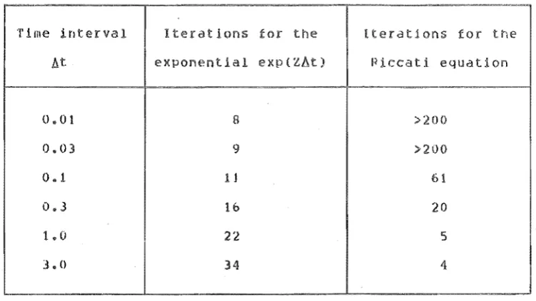
and techniques solving the matrix Riccati equation

are

Control of Proces

e

Discrete Systems

3 4 The ic Programming -to

Coni: Processes

3.5 Dynamic 'ehe Calculus of

Vax ions

3.6

al Solution of Hamilton-Jacobi

3.7 Newton~Raphson ut:Lon of tate

_Ri.

Equation

3.8 D of the

3.9

Kalman-Englar Techn

Page

34

36

38

40

42

44

46

47

CHAPTER III

DYNAMIC PROGRAMMING

3.1 INTRODUCTION

The dynamic programming appr to a variational

v~ry _{different that of the Calculus of} Variation

problem appears Instead of termining the entl extremal tra1ectory the dynamic programmlnq approach

i develop th~ e~tremal curve by evaluating the optimal derivative at each point, thus constructing an envelope of tangents. Where the Calculus Of Variations may be described as a global approach, dynamic programming is essentially a local approachq

The thpory of dynamic programmlnq was developed hy R.E.Rellman at the RAND Corporation in 1949 and the fir formal expository paper (Bellman,

was published by the National Academy of Sc ence U.S.A.

The intimate conn on betw dyn~ml proaramminq and Modern entral Theory was outLined by Bellman 961) and the ~pPllcation to con ro] p lems, a well as a very detailed bibliogr phy. has also been provided by

Bellman (1967,IQ711. For an introduct on to dynam c programming as qeneral optimisation technique the In erested reader should refer to the texts by Roberts (1964), Lapidus and Luus (1967), 8everidqe and Schecter

(1970), Boudarel, et aI, (1971) and ~oton (1972).

Dynamic proqra~ming is based upon the Principle of Optimality which may be stated as follows:

"an optimal policy has the property that whatever the initial state and initial decision the remaininq decisions must consltltute an optimal policy with regard to the state resultinQ from the first decision"

(1961,1967). Roberts (1964), Tou (1964), Lapidus and LuuI (1967), noudarel, et a1,(1971) and Noton (1972), Although there Is little merit in reproducing it in detail the technique may be demonstated by application to a simple stagewlse procels.

Before proceeding, however, i t

Is

necessary to define the terms to be used throuqhout thts section. The duration of the process Is divided into listaqes" corresponding to the discrete time interval and the stages are numbered in the direction of increasing time starting from stage zero. This has the minor disadvantage that the final stage of an N stage process is numbered N-1, but the advantages are substantial.

The "state" of the process Is the collectiDn of variables, expressed as a vector x, necessary to describe the condition of the process. !'Jhere

the state of the proce s may be observed only at the disc ete instants between stages the vector x

k Is defined as the state of the process at the beginning of stage k. The process thUS has initial and final stat s Xo and XN respectively and the proeess may be modelled by the linear equation

.. 0 1)

where <Vk and

11k

are the t ran .!. t ion i'lnd ell" i v ing ma r ie,,",!; propriat to staqe k and Uk is the control policy use throuqhout tage k

In qeneral terms the control criterion J(x,u,N-k) way be regarded as the cost incurred in traversing from ~tage k, state x_k' to the end of the control sequence uslnq a control policy u. If u is chosen to be an optimal policy the optimal criterion JD will be qiven by

.0 ...

(3.2) i

=

K, k+l, •••• , N

where N 1& the total number of stages in the sequence. If the cost incurred

In traver61nQ just the k"th stage is L(xk,uk,k). then the optimal criterion

may be expressed as

since the prine Ie of o~timal1tv states that the POlicy from stage k+l onwards must constitute an optimal policy using x

This Is the recurrence relationship and it wIll be seen that the multl-parameter optimisation of equation 3 2 has been reduced to a sinQle= parameter optimisation In equation 3.3 by imbedding the optimal solution for all the subsequent stages within the optimisation of stage k The sequence

may be initiated by establishing the terminal cost by calculus or Iterative techniques. An important feature of the recurrence relationshIp is that the optimal control policy is developed as a feedback law and this a will be demonstrated by the application to a linear fIrst-order

system.

• •••• 00000000000 •••••

3.2 CONTROL OF A LINEAR FIRST-OPDER PROCESS

Far the process descr bed by the equation

X kd the quadratic criterion

is to be minimised and the minimising sequence of controls r suits jn th~ optimal criterion

The cost for stage k Is

and the optimal criterion at the k"th stage may be ~xpressed jn recurrence

equation form

2

x

_N

with optimising control variable

The optimal terminal criterion may now be imbedded into the r@cu rence equation to solve for the final staqe.

min [ U ,J(

N-1

+ x2 ]

-1 N but from equation 3 4

.D.l0)

which i analytic

In

_{uN <,1} and the minimisinq control is fOllnd from

:;: _{0 .(3.11)}

q.ivlnq

LJ_N,,1 ( +b:2 ) , "( ) i N~'j 000.«0(.3«12)

and contlrming the rl(' CHl tj, ve l:eedrHlck tut'e of til€' cont t)} _law" TIle

sequencp is cant nued toward the origin with the optimising cont 01 qenerated as a equence of t edback qainsp eacI) approp late to it

independent ot the state at that staqe.

The combination of linear proce s and quadratic criterion produces an optimal criterion o~ quadratic form. e.q.

• 0 • • • ( .13)

and substitution of thi into equation 3 10 gives

mil'l[ x2 t ru1. + gk~1 (ax" ,,~ bll k)2]

u,<

1< Ie '"

and the right hand side is minimised for

.,Q"O (3.16)

which may be _{satisfied for all xk only it}

1 'I' r eoo • • (3.17)

Equations 3.15 and 3.17 define the iterative process for determining th sequence of feedback gain and optimal criteria. An important aspect, demonstrated later. is that the optimal crlt rion and the feedback gain converge to steady- tate values 88 N increases leading to constant

feedback gain for a p & with an unbounded tl

Fa a mult variable prace 5 wh eM may

d 1 s e t f 0 nil

and 1th quadratic criter on

,J t

k 01 ' < le! ~

lint" 1 Zan 0

lnodE'lled n the lInear

a tmllar iterative techniqup may be established to generate the sequence of linear multivarlable feedback matrices 8ecau e of the linear dependence of wl1l be strictly convex in u and unique minimum eXists p ovided the symmetric matrices S, Q and Rare positlve semiMde inite. As in the Single-variable example the optimal criterion may be assumed to have the quadratic form

' . 0 ••• (3.20)

The minimiSation of the right hand side of equation 3.21 is accomplished by partial differentiation with respect to each of the m elements of the control vector u_{1 ~} and minimising values are to be found from -the linear relationship

where the matrix Kk is obtainedlrom

SUbstitution of the optimising value of the control vector into equation

3.21 provides the optimal criterion

which may be rearranaed to give

.".".C].25)

Since the optinl~ll crlteri()n must be v;~11d for all xI< equation 3.,24 may be rearranqed to give

•••••• () 26)

and equations 3.22. 3.23, 3.25 and 3.26 define the iterative process from Which the sequence of control vectors Uk may be obtained.

With the criterion as defined by equation 3.1R the senuence would be injtiated by _GN

=

S. Where the steady-state feedback matrix is required, however, the initial matrix 15 of little sigrlificance and has no effect on the steady-state solution. Sufficiency conditions for the convergence of the matrix sequence have been presented by Caines and Mayne(1970) •

3 4 THE APPLICATION OF DYNAMIC PROGRAMMING TO CONTINUOUS PROCESSES.

For a continuous process described by the set of equations

,

l(

the process criterion may be expressed as the functional

The optimal criterion , at arbitrary time t and ate x, may be found by

the minimisation of the criterion with respect th~ control vector u. From the Prine Ie of Optimality the trajectory to the final time

t,

must be optimal and the c iterlon will be B function of both x and t, thus

min

rtf

=

u

J1

L (X.U,t)dt

t

••••• (3.29)

Xt the process Is opttml ov 1'10

the optimal

criterion

becomes

rt

5

f

J

f(}(pt)

-

min

_{u_}

:,U<0

. U_$t)r:lt -I- L(;<,u,t)dt

t+O

rnil'l

[

(l(,u,t)dt f(

,+xO,

t.5lJ

•• 0.30)

:::

1I +

..

wh<-!'re

[(

",tldt]

()«,-xO,t+5)

~ fnln L(x U

'hS

familiar form of the recurrence equation has emerqed Expressing

oo • • • • (3.32}

and for an infinj tesimal {5 the higher POWE'fS of {5 may be lanored. 'rhus

mi n

_u

[ I . '

_{r.. (}

_{x , u , t )9 t f ( x • t ) i}

at

a

f

5

₊

a

_§XX f,

5]

_{, , 0 0 .(3.33)}

but f(x,t) is not a function of the control vector u and may he removed from the minimisation. By dIviding throughout by {5 before allowinq it to nd

toward zero, results in

o

_::: mlh [ _{U T,(x,u,t)+ t}

_]

and the process mode]

,

)( provides the functional relationshir

between statp and control vectors to give

filill [

=

U L(x,u,t) + I.p(X,ll,t)]

which is the Hamilton-Jacobi ~quatlon of classical mathe~atlcal lIterature For the chosen c Iterion the houndary conditions are

O. hut for the more qpneral criterion ot equa ion

22 the terminal condi ion Is

f(x F [x (t )]

UnfortunAtely the analytical solution 0 thp Hamilton-Jacohi eQuation is ljmited to a few specjal cases where the tor~ of thP state equations and the criterion function result In a partIcular form at optjmal crjterion •

3.5 DYNAMIC PHOGRAMMING AND THE CALCULUS OF VARIATIONS.

Partial differentiation o~ the right hand side of equation 3.35 with respect to u and equating to zero defines the minimising control from

o

•••••• (3.36)

and substitution back into equation 3.35 completes the non-linear partial differential equation

• D . ] ? }

which provides the sufficient conditions for opti~allty (McCausland, 1969,

RellmClf), 19711.

Furthermore, dlvi5ion of equation 3.36 by the partial differential

0.30)

and SubKeQUent diff 10n.w th re pect to time

.(3 39)

Partial differentiation of equation 3.37 with r pect to x provide

o

9 U O • (3040)

and by combining equations 3.38 and 3.40, and subtracting from equation 3.39 prodllces

••••• (3.41)

whi.ch 5s tne Euler-Laqrange equation of the classical Calculus of

from Whlch

••••• (3.43)

and

!Q]

ax

t

(3 44)

The optimal traiec cry, denoted by the superscript Po", results in the optimal criterion

dnd from eQuations 3.43 and 3.44

H (XO , AO ,uo ) •••••• (3.45)

1I:'(t) .(3.46)

:~Ilbstitution into the Hamilton';'.Jacobi f'qllation (Jives

m~:1

[

t, ( )(" , U , t ) ~. H( ,uD₎

Of 0; H(

which imPlies that on an optimal traipctorv thp optima] value of u(t) Is that which a10bally minimises the Hamiltonian, which is a restatement of Pontryagin"s Minimum Prinriple •