A general algorithm for rational interpolation

A GENERAL ALGORITHM FOR RATIONAL INTERPOLATION

by

S. L. Loi

No. 33 June, 1984

1 INTRODUCTION

Recently Brezinski [1] presented a very effective general

extrapolation algorithm for linear and rational extrapolation. This algorithm was extended by Brezinski to a general interpolation

algorithm' which is called the Muhlbach-Neville-Aitken (MNA) Algorithm in [2] . In this rep9rt, the rational interpolating function is generalized in a similar way. This method answers the question raised in [2] by Brezinski. The aim of this paper is to present an algorithm for recursively constructing the interpolating rational function.

m

.1:

a.

i J=O J J ( 1.1)

R (x)

n m,n

.:E

m,n J J · i, i+l .•. i+m+n, i=O,l,2 ... ,

from either Ri

1 (x) orR 1i (x) by an extension of .the MNA

m,n- m- ,n

algorithm. The set of ·given functions [ {h. (x) } . mo, {h . ( x) f ( x) } . n 1]

J J= J J=

is assumed to form a complete ·or quasi complete Chebyshev system [ 7] on the set of interpolating points.

Instead of setting Ri (x)

. n,O 1 n

=

i R

0 ,n (x)

for the rational function (as in [2]), we apply this algorithm to the rational fraction Ri (x) directly.

o,n

i

Then the R (x) can be m,n

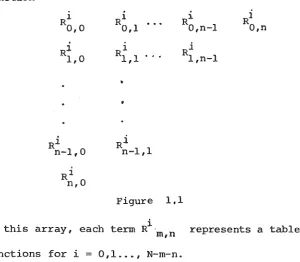
column horizontally. If (N+l) interpolating points are given, we could construct the following triangular array of the interpolating function

Rl Rl. Ri

0,1 O,n-1 O,n

1 _Ri

Rl,l l,n-1

Figure 1,1 i

In this array, each term R m,n represents a table of functions f o r i = 0,1 ..• , N-m-n.

This algorithm is more general than the algorithms suggested by Larkin [6]. With the normalization b = 1 Ri (x) is

0 ' m,n

expressed implicitly in the form

n . i

h

0 (x) R m,n (x)

i ~ .

'R (x).

1b.h.(x)+ m,n J= J J

m

.~

₀

]= J J

By using this algorithm, the coefficients of the inte:t;polating function can be determined easily. The interpolating value at a given point x=a can be found

( 1.2)

implicitly. However for computational convenience,.we could

transform the representation to a new basis

.h.

J J J

Vj

>

=

>

In Section 2 the MNA algorithm [ 2]is reviewed. The extension

of this algorithm to generalized rational functions is given in

Section 3. In Section 4 we discuss how to overcome the problem

when the algorithm breaks down due to a zero divisor. Some

examples and numerical results are given in SectionS.

2 THE MNA ALGORITHM

We begin by reviewing the MNA algorithm [2] .

suppose we construct the polynomials

he e ( f ) i

=

w r xi' i ~ ,

n

Then Pk(x) can be expressed as

0 -f -f k

n n+

n

g 0 (xn+k)

Pk (x) go (x) g 0 (xn)

gk (x) gk(xn) gk (xn+k)

D

Note: In this paper D is the minor obtained by eliminating the

first row and the first column of the determinant.

Now let gnk (x)be the ratio of determinants obtained replacing

I~

n

the first row in the numerator of Pk by

(-g. (x) -g. (x ) . . . -g. (x k))

J. J . n J.n+

n

i~k n

Note that gk . (x)

₌

=

.~ _{.~ J} ' 0 • • '

Then the MNA algorithm is the following

0 -f

n

n g

0 (x) go (xn) go (x)

P 0 (x) f

n

..

go (xn) go (xn)

-g. (x)

~ ·-g. ~ (x ) n

n go (x) go(xn) g. (x ) g 0 (x) _{- g i (x) ,. i.}

go,i (x)

=

go (xn) ~ n go (xn)

For k

=

=

n+l n n · n+l

gk-l,k(x) Pk-l(x) - gk-l,k(x) Pk-l(x)

n+l n

gk-l,k(x) - gk-l,k(x)

n Pk-1 (x)

n+l gk-l,k(x)

6. n

Pk-l(x) g n (x)

--- k-l,k

6. n gk-1 (x)

n+l gk-1, i (x)

n+k.

=

( 2. 2a)

n gk-l,i (x)

6. n

gk-1, i (x) n

gk-l,k (x) i k+l,k+2 ...

6. n gk-l,k(x)

and 6. is the forward difference on the.index n.

( 2. 2b)

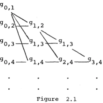
The way of computing gnk . (x) in [2] is equivalent to Aitken's

.~

...

pattern. With the initialization of gn

0 ,1. . (x) for a fixed value of

Figure 2.1

To show .the relationship to its generalization, this algorithm is essentially restated in a new notation.

For convenience, instead of using gnk . (x), we initialize

,J.

Note:

n

Vgl-k,k(x)

n Vgk,O(x)

n HgO,k (x)

is used. is used

We define Hg ~ k(x)

=

to generate to generate

-gk (x) go (x)

n Pk (x)

n Pk(x)

k = 1,2 vertically. horizontally.

and Vg ~ k (x) = 0 when j ~ k . -J,

Fori= 2,3,4 ... , j = 0,1,2 • • o I and k = j+i.

(2 .3a)

n

Hg . k(x)

- ) ,

n n+l . · n+l n

Hg_(j+l) ,k(x) Vg_j,k-1 (x) - Hg_(j+l) ,k(x) Vg_j,k-1 (x)

n+l n

Vg . k 1 (x) - Vg . k l(x)

- ) '

-

-n

6

Hg_

~+1)

n

6

n Vg . k(x)

- ] ,

n . n+1 n+l n

Vg_j,k-1 (x) Hg_(j+l) ,k(x) - Vg_j,k-1 (x) Hg_(j+1) ,k(x)

n+l n ·

Hg_(j+l) ,k(x) - Hg_(j+l),k(x)

n b. Vg -J, -

~

Vg_j ,k-1 (x) - - - Hg_(j+l) ,k (x)

where Hg ~ k(x) :

- ] ,

Vg n. k(x)'

- ] ,

-gk (x)

go(x)

9j+1 (x)

9k-1 (x)

-gk(x)

go(x)

gj+1 (x)

9k-1 (x)

-gk (x)

go(x)

9k-1 (x)

-gk (xn)

9o(xn)

9 j+l (xn)

9k-1 (xn)

9q(xn) (x )

9j.i-r n

.

gk-1 (xn)

-gk(xn)

9o(xn)

gj+l (xn)

9k-1 (xn)

9o(xn)

9 j+2(xn)

· 9k (xn)

-gk(xn)

9o(xn)

9k-l (xn)

-gk(xn+k-j-1)

9o<xn+k-j-1)

gj+l (xn+k-j -1)

9k-1 (xn+k-j-1)

9 o(xn+k-j-1)

gj+1 (xn+k-j-1)

.

9k-1 (xn+k-j-1)

-gk (xn+k- j-1 l

9o(xn+k-j-1)

9 j+l (xn+k-j-1)

9 (x . ) k-1 n+k-J-1

9o(xn+k-j-1)

9 j+2(xn+k-j-1)

.

.

gk(x k · 1) _n+

-J--g (x ) 0 n+k-j-1

9o(xn+k-j-1)

.

9k-l (xn+k-j-1)

0

( 2. 3c)

( 2. 3d)

( .2. 3 e)

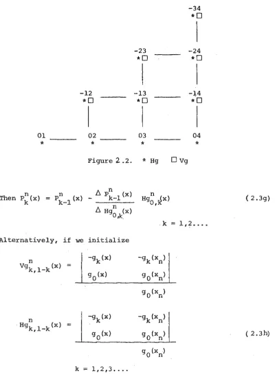
This is equivalent to Neville pattern and the way of computing can be shown by Figure 2. 2.

-34

*0

I

-23 -24

*0

*0

I

-12 -13 -14

*0

*0

.,. .. 0

I

I

01 02 03 04

*

*

_*

*

Figure 2 .2.

_*

0

Then _{Pk {x)} n

₌

-

P~-1

₀

6

Hg~

,]<;.,

. k

₌

n -gk (x) -gk(xn)

Vgk, 1-k (x)

go (x) g 0 (xn) go(xn)

n -gk (x) -gk (xn)

· Hgk, 1-k (x)

go (x) go (xn) ( 2. 3h)

then by using (.2,3c,d) to compute Hgk . (x) and Vgk . (x)

, - ] , - ]

we have

n

~

~

vg;,o

<x>

n

and Vgk,O(x) has the same form as (2.3f).

( 2. 3 i)

For linear interpolation, it is better to use the Aitken pattern rather than the Neville since it uses less storage and computation. But for the rational interpdation, Neville pattern is more effective and economical. The ratios of the differ~nces in ( 2. 2) and

(2.3b,c) are constant terms as shown in the following lemma.

LEMMA 1:

The ratio of the differences in

and

are

constants ( independent

of

Proof:

with the definition of Hg_(;+l) ,k(x) and Hg_;,k-l (x) in (2.3d,e) by using the Sylvester's identity and exchanging some

n

b. Hg_(j+1) ,k (x) ₌

n

b. Vg_j,k-1 (x)

9o (xn) 9 ₀ (x) _{9 o}1_{xn+l >}

.

. .

.

.

.

. .

.

9k-1 (xn)

' . 9 k-1 (X) 9 k-1 (xn+1) • 9 k-1 (xn+k-j-1) 0 1 0 • • • 0

,9

0(x) 9 o1xn+l)

. .

.

.

.

gj+2 (x) gj+2 (xn+1)

....

. . . .

.

. .

.

. .

9 k-1 (x) 9 k-1 (xn+l) 9 k-1 (xn+k-j)

1 0

.

.

...

0 1

'g 0 (x) 9 0 (xn+l)

9 j+2(x) 9k+2(xn+1)

0 • • • • 0

9 o<xn+k-j)

9 k+2 (xn+k-j)

...

9k-1 (x) 9 k-1 (xn+1)

1 0

-gk(x) -gk (xn+l) • • • -gk (xn+k-j)

9o<x> 9o(xn+l) . •

.

₊

.

.

.

. .

.

.

. .

.

.

9 k-1 (x) 9 k-1 (xn+1)

.

g

0(x n > 90(x) 9 0 (ic ,. ) , n+l 9

(X • )

0 n+k-j-1

gj+2(xn) gj+2(x) 9j+2(xn+l)~gj+2(xn+k-j-1)

-gk-1 (x)-gk-1 (xn+1) • .-gk-1 (xn+k-j)

( ) ( ) • • g (x-1+k-j)

· 9 o x 9o xn+1 • 0

9 j+1 (x) gj+1 (xn+l) • ' 9 j+1 (xntk -j) +

1

f

-gk-~

...

~j~l ~x~) .g:+~ (~) .g~+~ ~~n~l~ ·~j~1~x~+~-j-1)

J/

9 k-2 (xn) 9 k-2 (x) 9 k-2 (xn+l) "9 k-2 (xn+k-j-1)

-gk(x) -gk(x ) ' · • _n -gk~% _{n+ -J} k .)

9 o(x) 9 o(xn) • ' • 9 o<xn+k-j)

gj+2 (x) 9 j+2 (xn) • 9 j+2 (xn+k-j)

1 0 • • • 0

9 j+1 (x) 9 j+l (xn) · ' 9 j+l (xn+k-j)

9o(x) 9o(Y. ) • • .go(x _{n n+ -]} k .)

9j+2(x) 9j+2(xn) •• gj+2(xn+k-j)

9k l(x)-gk 1(x) ·-gk l(x k .) _{- - n - n+ -J}

l 0 • • • 0

where j + 2 <k

LEMMA 2:

k-1 (xn)

9 o(xn)

9j+l (xn)

• • - gk(x k .) _{n+ -J}

• 9 o (xn+k-j)

• • - 9 k l _- (x _n+. k .) _-J

9 o(xn+k-j)

9 j+l (xn+k-j)

The ratios of the differences in

and

are

constants

Proof:

=

constant

n [ .. n n ]

It is interesting to observe that gk-l,k(x) Vgk,O(x) 9 Hg0 ,k(x) . n

in the algorithm acts to increase the degree of Pk(x). The key

n [ n n

of this algorithm is to build up g .(x) Vg (x) Hg (x)] These k,l k,i , k,i

play an important role in the generalization ~o the rational interpolating function Ri (x) with Ri (x,) f.

m,n m,n J J

3 THE RATIONAL INTERPOLATION ALGORITHM

i

The interpolating rational function R m,n ( x) (. 1.1) may be expressed implicitly in the form (1.2). Then h i

0 (x) R m,n (x) can be expressed in the same form as ( 2.1) where f. is replaced

J by h

0 (xj).fj, j

=

gm+~(x)

=

h~(x)Ri

~

=

If we ass\.lllle gk(x) == xk₇k = 0,1 ••. m, gm+Q,(x) = x.Q_f(x),_t:::;: 1,·2 . . . n,

i

then R (x) can be expressed as below

m,n (3.1).

(Clearly a minor notational change will suffice to handle the more general case when h

0(x) is not identically 1).

i

R (x)

m,n

0

1 X

m ·x

-f. l. 1

X,

1.

m

X.

1.

n

X. f. l. l.

.

.

.

.

.

. . .

.

-f.

l.+m+n 1 xi+m+n

m X.

1.+m+n

X~ f. 1+m+n 1.+m+n

D

i

We can build up g (x) where m

=

( 3.1)

i i i

R

0(x), and g -" (x) where n = 1,2 ... for computing R0 (x) by

m, n-~,n ,n

using ( 2.2) which is based on Aitken's pattern, or build up

i i i i )

Vg

0 (x) for R 0 (x) and Hg0 (x)for R (X by using ( 2. 3) which is

m, m, ,n O,n

based on Neville pattern. Then by using the relation of Vgmi,O(x) (gi

1 (x)) and Hg0i (x) (gi (x)) we build up

Vgi (x) and Hgi (x) which is based on Neville's pattern for

m,n m,n

constructing Ri (x) either from the previous column or row. The m,n

following algorithm is based on the Neville pattern. 1. Initialization.

For m,n = 1,2, ... Nand fori

i

Vg

1 (x)

m, -m

i

Hgm, 1-m (x)

where go (xi,) = 1 m g (x.) X. m i

m l. l.

i Vg

1 -n,n (x)

i Hg

1 -n,n (x)

where _gn (x.) x.f. n

l. l. l.

go(xi) 1 n =

0,1, ..• , N-1

~-gm

I

-gm (x) go (x)

1,2 0,1

~-gn(x)

I

1-g (x)

I

g:

1,2

...

-g (x.)

I

I

go (xi~

-g (x.)

I

go(xi) go(xi)

-g (x.)

I

n 1

I

go(xi) go(xi)

-g (x.) _{n l.}

I

l

( 3 . .2a)

2 . For k

=

Form= N, N-1, ..• ,k-N

set

Fori= 0,1, .•• ,N-k

i

Hg (x) m,n

i

Hgi

1 (x) - b:. Hgm-1 ,n (x) · Vgi 1 (x)

m- ,n

m,n-i

b:. Vg

1 (x)

m,n-( 3. 2c)

i Vg (x)

m,n

i = Vgi

1 (x) - b:. Vgm,n-1 (x) H i ( )

m,n- gm.,.l ,n x

i

b:. Hgm-1,n(x)

( 3. 2d)

3. For i =

o,

0,0(x) = fi For n 1,2, ... ,N

For i Ri ( x)

O,n

· o,

.

tm

o,

1

0,n-1 (x} - i Hg O,n tx)

~Hg O,n ( x) Form= 1,2, ..• ,N

Fori= 0,1, .•• ,N-m

i ) i ('

R m, 0 ( x = R m-1, 0 x) -i

~R m-"-1 _, 0 ( x) _l. ·

i Vg m, 0 ( x)

~Vg

0 ( x) m, For m,n ~ 1,2, ... N

Fori= 0,1, •.. ,N-m-n

Ri (x) m,n

i b:. R i

1 (x) i Rm,n-1 (x) m,n- Hg (x)

i m,n

b:. Hg (x) m,n

( 3. 2e)

Ri (x) m,n

i b:. i (x) i

(x) R

R

-

m-l,n

i m,n

'b. _{Vg (x)}

m,n

( 3. 2f)

THEOREM 1

Equations ( 3. 2e) and ( 3. 2f) hold for m,n 0' l ' 2 . . . .

provided n

>

>

Proof: To prove i

(3.2e), using the Sylvester's identity for the determinants, R (x) can be decomposed as the. following:

m,n

1

0 -f. l. 1 1

X _xi

m m X x.

l. xf x.f.

l. l.

-f i+m+n

1

X~ _J.+m+n

xi+m+nfi+m+n

n-1 n-1

xi fi • • xi+m+nfi+m+n

1

Ill

X.

l.

1

m xi+m+n

x? f J.+m+n i+m+n

.

D

-f i+m+n-1

.

xi+m+n-1

.

.

m xi+m+n-1

xi+m+n-1

1

X l\i

..;

..

1

x.f. l. l.

fi+m+n-1

1

n-1 . n-1

i

Hg (x) =

m,n

n -x f

X

m

X

xf 1

n -x. f.

1. 1. 1

n

.-x. _l.+m+n-lf. _1+m+n-1 1

• xi+m+n-1

m m

xi ' • • xi+m+n-1 x.f.

1. 1. X. l.+m+n-lf. 1.+m+n-1

n-1 n-1 n-1

X f X, f. •• :X f

1 X,

1.

m :x;i x.f.

1. 1.

n-1

X. f.

1 1

• . 1 . 1

~ 1. 1.+m+n-

l.+m+n-.

.

.

.

• x.

l.+m+n-1

m

xi+m+n-1

x. _J.+m+n-lf. _1+m+n-1

n-1

• • • X, lf, 1

1.+m+n-

1+m+n-( 3. 2g)

which is the second factor of the second term by shifting the last row to the first row and change the sign. The first factor of the

i

6. Rm,n-l(:x) s.econd term is in fact equal to

i

6. Hg (x)

In the same way as in lemma 1, it ·can be shown that

i /;;,. R

1 (x)

m,n-i /;;,. Hg (x)

m,n

-f. 1. 1

X.

1.

m X.

l. x.f.

l. l. .

.

n-1

x.

l. l.

n

-x.f. 1. l. 1

X.

l.

m

X. 1

x.£. _l.

J.

n

x.f. _{1. l.}

"

..

-f. 1.+m+n 1 X.

1.+m+n

m

X.

J.+m+n

X. f,

l. +m+n 1. +m+n

n-1

x. f. 1.+m+n l.+m+n

n-1

-x. f.

J.+m+n l.+m+n 1

x.

J.+m+n

m

X.

1+m+n

X. f,

1+m+n J.+m+n

n-1

X. f.

J.+m+n J.+m+n which is a constant fanned by the interpolating set

{(x.,f.), j

=

J J

To prove (3.2f), shift the mth row of the numerator in ( 3. 1 ) to the last row and the proof follows using the same method as above, where in this case .the second factor is defined

i

Where we define

i

Vg (x)

=

n -x .f

l

X

m

X

xf

n-1

X f

n

-x. _{l. l.} f. • ·• 1

.

.

.

. .

.

m x.

l.

x.f.

.

.

-J, l.

. .

.

n-1

X. f.

.

.

l. l.

n f

- xi+m+n-1 i+m+n-1

1

x. _l.+m+n-1

.

m ,

X. _l.+m+n-1

.

~ +m+n- l.

+m+n-. +m+n-. +m+n-.

.

n-1

~ x. 1f. 1

l.+m+n-

1.-~t'm+n-(3.2h)

Note: 1.

1 II p A o

X. l.

m-1

x.

l. x.f.

l. l.

n

x.f. l. l.

.

.

• xi+m+n-1

m-1 xi+m+n-1

X _{i+m+n-1 1.+m} f,

+

n

x. _{1.+m+n -1 1. +m+n-}f. 1

i i

The expressions for Hg (x) and Vg (x) have common

m,n m,n

numerators and the denominators have one row different. 2. The expressions for Hgi

1 (x) and Vgi 1(x) have

m- ,n .

m,n-the same denominators but m,n-the numerators have one row different.

THEOREM 2.

Equations (.3 .2c) and ( 3 .2.d) hold for all integers m,n

such that m + n

>

COROLLARY 1.

The ratios of the differences in ( 3. 2c), \3. 2d), ( 3. 2e)

and ( 3. 2f) are constants (independent of x).

Proof:

i i}R ·

1(x)

m,n-Consider----~---­

/:::, Hgi (x)

, - the ratio of the differences in

m,n

( 3.2e). From the proof of Theorem 1 i t is clear that the ratio

is a constant term ( independent of x ) . The proof for the other

ratios follows similar1y.

GOROLLARY 2 • i

Hg (x) =

m,n

Proof:

i

k., Vg (x)

1 m,n where k. ₁

tiHl

m-l,n i

Avg (x)

m,n-1

T})is follows immediately by combining ( 3. 2c) and { 3. 2d)

since the ratios of the differences are inverses and, by

Corollary !,constant.

COROLLARY 3 •

In the case h. (x)

=

J xj , the maximum degree3 ky of the terms

k

.x and x R (x) in Vg (x) and Hg (x) are

m,n m,n m,n m and n

respectivel-y.

Proof:

From the initialization ( 3.2a,b) i t is clear that the degree

of

f

1 (x) is m and the degree, k, of

m,l-m m, -m ·

k i . i

x R in vg

1 -n,n (x) = Hg. -n,n 1 (x) is n. By induction using k

(3.2c,d) and Corollary 1, the maximum degree of x in

i i k

Vg (x) and Hg (x) is at most m.Similarly for x R

i i+l

COROLLARY 4.

If

=

then

(where

1,

,has

m,n m,n l. 1.+

b

een

in Corollary 2) and

=

m,n m,n

Proof:

m,n m,n

i i+l i+l i

Hg

1 (x)Vg 1(x) - Hg 1 (x)Vg 1(x)

m- ,n m,n- m- ,n

m,n-i+l i

Vg .l (x) - Vg

1 (x)

m,n-

m,n-=

Hgi+l (x)Vgi+2 (x) - H i+2 (x)V i+l (x) m-l,n . m,n-1 gm-l,n gm,n-1

. +2 i+l

Vg1 (x) - Vg

1(x)

m,n-1

m,n-i+l i+l

By cross multiplying and inserting- Vg

1(x)Hg 1 (x)

m,n- m- ,n

in both sides, i t follows

. '+l '+1 .

~

1

(x)~

1

1(x)

=

~

1

1

(x)~

1

1(x).

m- ,n m,n- m- ,n

m,n-i Hence k

=·

i i+l m,n

i+l Vg (x).

·m,n

Note. All these results follow in similar way for the general case k

when x.

l.

k

is replaced by h (xJ..) and x.f. replaced by h (x.)f .. -k l. l. "1< l. l.

4, THE SINGULAR CASE

These algorithms may break down if the adjacent terms are equal.

. i+l i

For examp.J_e ~ Hgm1,n-l (x) is zero i f Hg

1 (x) = Hg 1 (x).

m,n-

m,n-i+l i

Then since Vg .

1(x) = Vg 1(x) from Corollary 4, i t follows

m,n-

m,n-i

Hg (x) = 00

m,n

i

and Vgm+l,n-l (x)

i

In the case noted above, the indeterminancy of Hgm,n (x)

j

implies that

h

j

Hg (x) for j

=

cannot be computed. This difficulty may be overcome by jumping two steps. Instead of ( 3. 2c) it can be shown

i i-1 , i-1

Hg

1 (x) Hgm,n (x)

- 6

mt· ,n

i i+l

- /J.g. Vg i+l

Hg (x) Hg (x) (x)

m+l,n m,n m+l,n-1

where if m

=

=

where i-1

Hg +l _{m ,n} (x) Hg

i-l

1\ i-1

w Hg (x)

- m,n

6 i-1

Vg _m+ 1 _,n-l(x)

( 6 Hgi

1 (x)

i-1

Vgm+l,n-1 (x)

m- ,n

I _

= Vg!,n-l (x)\

6

6. Hgi-11 (x))

A i-1

, w Hg (x)

₆

( 4. la)

( 4.lb)

b. · m,n

g : _J.-' 1

6. Vg .1 l(x)

m+

,n-

6

i-l

\

,

f>g

If Vgi · 1 (x)

m,n-6 Hgi

l

6. _Vg i·

1 2 (x) m+

,n-. 6 Hgi (x)

m,n-1 8 Hgi-1 1 (x) m,n- )

Hgi

1(x) for all i. Then

m,n-6 Vg i-1 - 6 Hgi-] (x) 1 (x)

m,n- m-l,n

6 _Hg i-1 _{. 6 Vgi-l (x)} 1 (x)

-m,n- m+l.,n-2

6 _{Vgm,n-1 (x)} i 6. Hg i

1 (x) m,n-When 6. Hgi

1(x) = 6. Vgi 1(x)

m,n- m,n- 0, the above form can be reduced to

A i-1 w Hg (x)

m,n 6. i-1

· Vgm+1 ,n-1 (x)

i 6 Hg

1 (x)

m- ,n i

By the same method it can be shown

!J. Hgi 1 (x) m- ,n

( 4. 2a)

[), v

m+l,n-2 x

This applies to the case when the singularity occurs at the first step. i.e. k Q 2, otherwise more work is required to derive !J.g

=

i

!J. Hg (x)

m,n

!J. _Vg i _{1 1} ( _x)

m+ ,n-i

!J. Hg (x)

m,n

=

[), _Vg i _{1 1} ( ) _X

m+

,n-!J. _Hgm-l,n(x) i+l

•

·as follows:

i+l Vg

1(x)

m,n-H it1. (x) 9_m,n-l

!J. Vgi (x)

m,n-1 - !J. i

( x) !J. i+l

Hgm-l,n Vg m,n-1 (x)

!J. _Vg i+1 _{1 2(x) !J. Hgm,n-1 (x)} i - !J. _Vgm+1,n-2(x) i !J. _Hg i+1 _l ( ) X

m+ ,n-

m,n-!J. Hgi (x)

m,n-1

i

!J. Vgm,n-1 (x)

!J. H ₉i+l (x) m,n-1

A i+l

u Vgm,n-1 (x)

where !J.

Hg~,n-1

X

i+1 Vg

1 (x)

m,n-!J. Vgi 1 (x) !J.

m,n-( !J.

Hgm~1,n-1

vi:+l

2

m,n-2 m,n- !J. V i+1 9_m,n""'2 (x)

- i+l i

Hgm-1,n-l (x)(:

Vg~,n-2(x)

V i+2 (x) 9m,n-2

Hgm-1,n-l (x) . i+2 (

Hgm-1 ,n-1 (x) !J. Hgm-1,n-1 (x) i+l

!J. Hgi+1 (x) !J. Hgi+2 (x)) m-1,n-1 - m-1,n-l

!J. Vgi+1 (x) !J. Vgi+2 2(x)

m,n-2

m,n-i+1 i+2

!J. Vg _{m,n-2 (x)} !J. Vg _m,n-2 (x) )

i+l i+2

i+l i+2 _6. i . Vg

2 (x) Vg 2 (x) Hgm-1,n-1 (x)

m,n-

m,n-. i+l i+2 _6. i

Hgm-1,n-1 (x) Hgm-1,n-1 (x) Vg _m,n-2(x)

m-1,n-1

(6.

l

6. i+2 ( ) Hgm-1,n-1 x

i+2

6. Vgm-1,n-2(x)

I£6. _{Vgm,n-1 (x)} i i

6. Hg (x) m,n i

6. Vgm+1,n-1 (x)

i+1 Vg

2 (x) m,n-i+l

Hgm-1,n-1 (x)

6. _{Hgm,n-1 (x)} i 0, then

6. _{Vgm,n-2 (x)} i+l 6. _Hg i _{1 (x)} m- ,n 6. _{Hgm-1,n-1 (x)} i+l 6. _Vgm+1,n-2(x) i

i+2 Vg

2 (x)

m,n-i

6. Hgm-1,n-1 (x) i+2

Hgm-1,n-1 (x) 6.v/ _m,n-2(x)

(

:

Hg~~~,n-1

2

i+l Vg

2 (x)

m,n-i+2

6. Hgm-1,n-1 (x) 6. _Vg i+2 ( )

2 X

m,n-6. 6.

After the terms rearrangment, these can b~ expressed as

6.g = -6.1 .6.2 .6.3 where _{Vgi+1 (x)}

6.1

₌

'

,

i+l Vg

1 (x) m,n-i+l Hgm,n-1 (x)

( 4. 2b)

i

6. i 6. i+l

!:::,. Hg. 1 (x) _{Hgm-1,n-1 (x) Hgm-1,n-1 (x)}

6.2 =. m- ,n

i+1 i i+l

Hgm-1,n-1 (x) !:::,. Vg

2 (x) 6 Vgm,n-2(x)

m,n-6.

v

9m,n-1 gm,n-2 Hgm-1,n-1 (x)

6.3

=

·•

and by the same method,

where

A

i-1

u Vgm,n-1 (x)

i

Hgm-l,n-1 (x)

if k = 3,4, ••• N

i-Vg

2 (x) m,n-i-1 6 Hgm,n-l(x)

( 4.2c)

i-1

6

6vg

2(x)

m,n-The computation of Vgj (x)

m+l,n 1 j

=

I I

the terms 6g and

6g

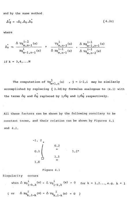
All these factors can be shown by the following corollary to be constant terms, and their relation can be shown by Figures 4.1 and 4.2.

-1, 2

*

(

0,1 1,2*

1,1

0 (X)

1,0

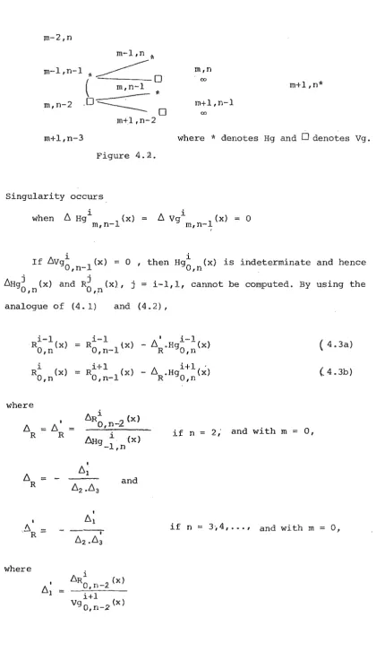
Figure 4.1 Singularity occurs

when 6 i . (x} !3. i (x} 0

Hgl-k,k = Vgl-k,k == for k 1,2 ... , e.g. k-= 1

6 i

m-2,n

m-l,n

*

m-l,n-1

*~

(

- - - - 0 m,n-1 *

0~

m, n-2 ·

-0

m+l,n-2

m,n

00

m+l,n* m+l,n-1

00

m+l,n-3 where

*

Singularity occurs when 6 Hgi

1(x)

m,n- 6 Vgi m,n-, 1(x)

=

If 6vg;,n-l (x)

=

0j ,n (x) and R0j ,,n (x), j

=

i-1 R

0 ,n (x)

i R

0 ,n (x) where

6

₌

6 = R

I

./:). _{. R -}

-where 6

I 61

'

i-1 I i-1

RO,n-1 (x) - 6 R.HgO,n(x)

i+l i+l .

= RO,n-1 (x) - 6 R.Hgo,n(x)

6R;,n_₂ (x)

=

6Hg i (x) -l,n

if n 2,· and with m 0,

I

61

62 .63 and

I 61

if n 3~4, ... , and with m

/:; i

RO,n-l(x) i+l VgO,n-2 (x)

( 4. 3a)

( 4. 3b)

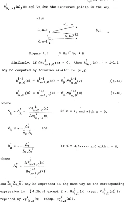
Figure 4. 3 shows how the calculation of R 0

i (x) involves ,n

i

RO,n-l(x),Hg and Vg for the connected points in the way.

-2,n

-1, n

- - - .j(

-1, n-1

____.--(* - - - o

D - e - - · - - *

O,n

*

0, n-2.

0

Figure 4.3

*

then Rm,O (x), j

=

i-1

( 4. 4a) R

0(x)

=

m, m,O

Ri (x) = Ri+l ~ x)

-

rn,O rn-1,0 R rn,O

where

•

R R _i

fl.Vgm '-1 (x)

if m = 2, and with n

=

o,

II

fl

--

/j,2 ·/j,3

I II

/j,

₌

R _{- u}

~2 ·/j,3

if m 3,4, ... , and with n

_o,

where

-

-

-'

and /j,2 .6.3 /j,3 may be expressed in the same way as the corresponding

1 '

i

expression in ( 4. 2b, c) except that Hg b (x) a,

i i

replaced by Vg b _,a (x) (resp. Hgb _,a (x)).

Figure 4.4 shows how the calculation of R i

0{x) involves m,

i

Rm- 2 , 0 (x), Hg and Vg for the connected points in the way .

•

~----o

m-1,~ .,. m-1, -1 0 - - - - ·

---

0

Figure4.4

In fact the above expressions ( 4. 3) and

·m,o

( 4. 4) can be

i

generalized to computeR (x) for m,n = 1,2,3 ... where some of m,n

i i

R (x) do not exist. But in this case R (x) may be generated

m,n m,n

either 'horizontally' or 'vertically' (3.2e,f). If the calculation is blocked one way then i t is possible to continue in the other way. Thus the situation is simpler than (4.3) and (4. 4)

This approach was motivated by the method used by Wynn [11] to deal with the singular cases.

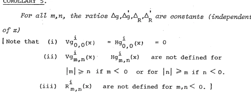
COROLLARY 5.

I I

For all

the ratios

are

(independent

of x)

[Note that {i) _vgo,o<xl i _Hgo,o<x> i

₌

i i

Vgm,n {x). Hg (x) m,n

(ii) are not defined for

Proof:

(4.2b)

Only the first ratio ( i.e.

i

b. Hgm-l,n(x)

i+l

Hgm-l,n-1 (x)

)

for m and n ~ 0 is proved . The others· follow in a similar way.

From ( 3.2g,h),

i

b. Hg

1 (x) m- ,n i+l Hgm-l,n-l(x) -xn! 1 X m-1 X xf n-1 )( f

-xn f i+1 1-+1.

l. xi+1 m-1 xi+1 xi+lfi+l

. .

.

xi+1fi+1

. .

0i+1 m-1,n

-x~ f.

l.+m+n-1 J+m+n-1

• q 1

xi~~+n-1

m-1 xi+m+n-1

n-1

xi+m+n-1fi+m+n-1

n-1 n-1

-x f -xi+l fi+1

1 1

X

xi+1

m-1 m-1

X

xi+1

.

.

xf _xi+lfi+l

.

n-2

X f _xi+lfi+l n-2

..

. .

.

i m-1·

where 0

m-l,n X, l. •

I

-.

.

n-1

x. f. I'

l. ~

.

'

.

.

1 1

X

m-1 m-1

x xi

n-1 n-1

x fx. f .• l. l.

n-1 .n-1

-x~ f. l.+m+n-2 l+m+n-2

1 m-1 xi+tn+n-2 xi+m+n-2fi+m+n-2 n-1 ·xi+m+n-2fi+mtn-2

-x i+m+n-·2t i+tn+n ·2

1

x i+m+n-2

.

m-1 xi+m+n··2

xi+m-l-n-2f i +m+n-2

.

n-2

xi+m~n-2f i+mtn-2

1 xi+m+n-2

.

.

.

n-1

By applying Sylvester's identity to the determinants and exchanging

some rows or columns, then

- x~f. ~ l.

1 X. l ni-l X. J. x.f.

l. J.

n

-x f _{-xi+1 fi+l} . n

1 1

X _xi+1

m-1 m-1

x xi+l

xf xi+1 fi+1

n · - xi+m+n-1

·

..

xi+m+n-1 m-1 xi+m+n-1 xi+m+n-1fitm+n-1 1 X m-1 X xf 1 x. l.

X. f,

J. l.

1 m-1 xi+m+n-2 · m-1 xi+m+n-2 x itm+n-2f'i+m+n-2 i+1 n-1 xi+m+n-1fitm+n-1

.. · · · · 0rn-l,n-l

0 1 0

.

.

Di

m-1,n 1

X·

m-1

X

X f

n-1

X f

n-1

• x. _J.tm+n-2f. ~+m+n-L ~I

1 1

m-1

x. _xitn.tn-2

J.

m-1 m-1

x. _xi+m+n-2

J.

x: f.

~ l. · xi+m+n-2f i+tn+n-2

.

n-1

xi fi. _{xi+m+n-2fi+m+n-2} n-1

After eliminating terms this is easily seen to be a constant term.

Using (2.3d,e) and the same method i t is straightforward to

extend the result to the cases m<o or n<o.

S.NUMERICAL RESULTS

It is obvious that when x

=

general rational extrapolation. since the interpolating functions

which are generated by this algorithm have the implicit form

interpolating function value at a given point, especially when done by the computer. But if thls point x

=

x'= 0 and the interpolation algotithm· is used, the arithmetic is substantially simplified.

Example 1.

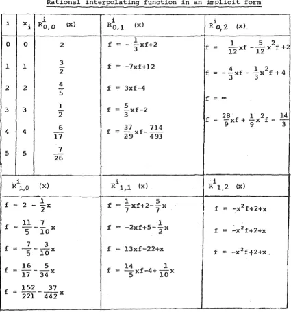
The same example is used as in [4].

Table 5.1

Rational interpolating function in an implicit form

i X. _Ro, i

_o

Ro,1 (x) Ro2 .(x)

l. _I

0 0 2 f

=

-

₃

1 1 3 f

=

2 _{f = - - x f - -x f + 4}

3 3

2 2

-

f ::: 00

1

f 5

3 3

-

=

2 3 _{28 1 2} 14

f = -xf + -x f -

-6 37 714 9 9 3

4 4 f

=

2·9 xf- 493 17

5 5

-

26

. i

(x) Ri (x) . i (x)

R 1,0 1,1 R 1,2

f

=

=

f+2+x

7 ' 7

=

f

=

=

15

=

f

=

f -:x2ft2+x.

5

f = _l7-34x 16 5 f

₌

____ _j

(continued.) i

R 2,0 ('x )

i

R 2,1 ( x)

i

R 2,2 (x)

2 1 2 _{1 . 3 x}2

-x2f+2+x f

₌

₌

.5 10 _{2 2 4.}

13 13 1 2 _f 7 5 x2 _{f == -x}2

f+2+x f = - - - x _+~

=

-5 10 6 6 12

33 7 X 2

158

₅₈

--x£+17--x+-f ==

₈₅

292 163 7 2

f

₌

- - -

.where f is the rational approximation

These results are exactly the same as those obtained explicitly in [ 4] .

i i

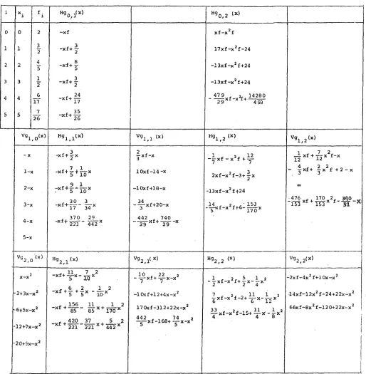
The terms Hg (x) and Vg (x) for the construction or the

m,n m,n

table 5.2

i X. _l f. HgO! l(X) Hg0,2 (X)

l

0 0 2 -xf xf-x2f

1 1 ₂ 3 -xf+ ~ l7xf-x2f-24

2

2 2 4 ₅ -xf+ ~ -13xf-x2 f+24

5

3 3 ₂ 1 -xf+.:!. -13xf -x2 f+24

2

4 4 6 -xf+ 24 479 f 2t 142aO

17 17 - 29x -x +493

5 5 7 35

126 ~f+ 26

Vg1,0(X) Hsl,1(x) Vg1,l (x) Hgl ,2 (x) _{Vg1,2 (x)}

-x -xf+~x 3.xt -x

-~xf-x2_{f +}12 1 7 2

2 3 I2 xf + 12 x f-x

7 7

1-x -xf+ Z. t .?:._x lOxf-14 -x

2xf-x2_f-3t-~x

·-

2

f +2 -x

5 10 3 3

2

2-x -xf+2~.?:.._x -10xf+la-x "'

I 5 10 -l3xf-x

2

ft24

-xf+~- ~x -.:!!xf+20-x

.:.476 t+ 110 2£.£19-x

3-x _-~=i1<f-x2_{ft6~ ~x} 153 X 153 X .51

17 34 3 _{5 170}

4-x -xft 370- 29 -~xf+ 740 -x

221 442 X _{29 29}

5-x

Vg2,0'(x) _{Hg2,1 (x) Vg2,1< .x) Hg2,2} (X) Vg

212(xl

2 11 7 2

-10 xf+ ~x-x2

x.,-x -xf+ ₅ x-₁₀x

-~ l<f -X 2 f + ~X-!_X 2 -2xf-c4x

2

ft-10x-x2

7 7

-xf+.§_ +lx -l....x 2

2 2 4

2+3x-x2

5 5 10· -1 Ox f+l2+4x -x2

lxf-x 2 _f-2+ ~x-_{.!___ x}2 J4xf-12x

2_f~24+22x-x2

-xf + 156 _ 11 1 2 6 6 12

I

6t5x-x2 as x+ 170 x 17 Oxf-312+22x-x

2

~xf-x2_{f-15+ ~X'-!.x}2 66xf-8x

2_f-120~22x-x2

I

as

442

xf-16a+ 74 x-x2 4 4 8

I

420 37 5 2

-12+7x-x2 -xf +m-221 X+ 442 X 5 5

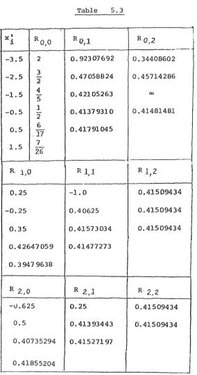
Numerical rational interpolation at x == 3.5, computed by transforming x = 3.5 to x'

=

Table 5.3

x'

_Roo

!

i I I I

~-·--3.5 2

o.

2

-1.5

-

5

-0.5

_-

0.5 6 0.41791045 . 17

1.5 7

26

R l,O RJl _I R 1 2

'

0.25 -1.0 0.41509434

-o.

0. 35 0.41573034 0. 41509434

0. 42647 059 0.41477273 . 0. 3 947 9638

R 2 0 I R 2 1 , R· 2,2

-0.625 0.25 0. 41509434

0.5 0.413 93443 0.41509434

0.40735294 0.41527197

0.41855204

Example 2. 2

Since Hg O, l (x)

Hg~'

Hg~

₁₂

(x).

R~,l

Table 5.4

i X. f. _{HgO,l (x) Hg0,2(x)}

~ l.

0 0.5 2 -xf+l 23 2 9

10xf-x f-5

1 2 3 -xf+6

xf-x2f+6

2 4 o.s -xf+2

"'

3 1 2 -xf+2 4xf-x2f+6

4 3 2 -xf+6

Vgl,O(x) Hgl,l (x) Vgl,l (x) Hgl,2(x) Vgl, 2 (X)

0. 5-x _{-xi- 3+ Tx} 2 10 lOX 3 f +0.2-X 87 2 51 3 9 87 24 2 51

48 xf-x ·f-24 + 24x 78 xf- 39x f-t 39 -x

2-x -xf+l0-2x - ~xf+S-x

2 2xf-x2f-4+2x xf -0. 5x < f-2 tx

'

4-x -xf+2 00

3xf-x2 f-6+2x 3 1 ~

2xt-2x. f-3+x

1-:x -xf+2x ~xf-x

2

3-x

i i

R (x) can be computed either from R

1 (x)

m,n m- ,n

i orR

1(x)

m,n-Table .5.5

i X, _{Ro,o(x) R0,1 (x) RO, 2 (x)}

l

0 0.5 2 1 9

f 99 17 " 63.

f

=

-

= 104 xf- 52 xLf+

₅₂

5 5

l 2 3 5 6

f 7 . 1 2 3

f

=

f+-8 8 8 4 4

2 4 0.5

'1 2 1

00

f == xf--x

f+-1 2 4 2

3

f

=

4 3 2

Rl,O(x) Rl,l (x) Rl,2(x)

5 2

f 23 61 51 5 1 r 25 2

f

=

₌

₌

3 ·3 64 32 96 24 12 12 3

11 5 3 7 l 5 1 2 5 l

f

=

- -

=

8 _{8 8 4}

₄

5 1 1 1

f =

-

-

-

2 f = 2

Example 3.

i ' In this example f (x

2). == 0 and hence RO, 1 (x) , i == l, 2 and

R~

=

'

Hg~

₁

(x)

Hg~

Vg~,l(x)= Vg

1

~

1

0 0 0

·at Vg

211(x) and Hg112(x). Hence l).,l (x) does not exist. Note that the algorithm continues to calcul·ate higher order interpolations

Table 5.6

i _{xi fi Hg0,1(x) Hg0,2 (x)}

0 1 4 -xf+4 -x2!+4

1 2 1 -xf+2 2xf -x 2 _f

2 3 0 -xf 4xf-x2f

3 4 1 -xf+4 _17 xf+x2f- 20

3 3

4 5 2 -xf+lO

Vg1 ,0 (x) Hgl,1(x) Vg1,1 (x) Hg (x) Vg (x)

1,2 1,2

·1-x -xf+6-2x -2 1 xf+3-x ClO -~xf+-3-x

2

1 1 0 _{x f -x} 2 f -8 + ~ _{x -} ~xft ~x2f+3-x

2-x -xf+6-2x - 2xft3-x _{3 3 .} 4 8

3-x -xf-12+4x !xf+3-x

9xf-x2f+60-2x ~xf-

.J:.

4 _{20 20}

4-x -xf-20+6x ~xtt₆ 10₃ -x

5-x

vg2 , 0 cx> Hg2,1 (x) Vg2,1 (x) Hg2,2 (x) Vg2 ,2 (x)

4xf-x2f-24+14x-2x2 ' 1 2 2

-2t3x-x2 -xf+6-2x _"' 2xf- 2x f-l2+7x.ox

-6+5x-x2 _{-xf+24-17x+3x} 2 _{!.xf-8+ 17 -x 2}

!xf -x 2f+60- 91.x+ 17 x2 1 2 2 12 0 91 2

3 3 2 2 2 -17xH17x f-17t 17x-x

l2t7x-x2 _{-xf -3x+x} 3

·xft3x·-x2

i x. R (X)

l. o,o

0 1 4

1 2 1

2 3 0

3 4 1

4 5 2

R

1, 0 tx)

'

f

=

f

=

f = -3+x

f

=

R. 2 o(x)

_,

f

=

f

=

f

=

Table 5.7

RO 1 (X)

'

3 f

=

2

f

= -

4

f ;::: - +- xf 1 1 3. 6

R 1,1 (x}

00

f

=

R2,l(x) f

=

1 5 1 2

f = -xf-3+ -x- -x

2 2 2

R o 2'(x)

'

3 1 2

f = -::-xf- -x f 2 2 3 1 2

f = -'Xf- -x f

4 8

f

₌

R 1 2 {X)

'

1 2

f

=

f 9 1 2 9 '3

=

17

+

17-

17

R2,2 (x)

f

=

7 7 7 7

Example 4.

If x. is considered for i

=

1

interpolating functions ·may be expressed explicitly. Then

0 4-x

R

2,1 (x)

= --

functions which can be expressed as continued fractions. Note that

x₂ = 2 is considered as an 'unattainable point' of R0

1 (x} (see [ 10] )·. 2,

If the method suggested in [3] which reorders·the

points so that the 'unattainable points' appear at the end of the

list is used, then

4-x

2 and

0

Rl,l (x) 14-Sx _7-x

In this case x

3

=

algorithm terminates.

With the algorithm described in this chapter, all possible

forms of the .interpolating function may be computed and decided

which is most suitable. Even when more points are added, the

interpolation procedure may still be continued without reordering

the points and higher order functions may be obtained. For example

if f (4)

_{= .}

17 1s added, then R2 , 2 (x)= l+x~ ( see Example 1)

2.

Alternatively suppose f(4) = 1 is added, then RO (x) 96 - 62 x+llx

2, 2 48-22x+4x z

Both of these functions interpolate f(x) at all the points x.

1

i = 0,1,2,3,4 despite the existence of unattainable points for

Example 5. (Example 3 in l3]).

If f is infinite at one of the interpalation points, It can be replaced by a parameter a, in the computation.

Suppose f(O) = l, f(l) ~ ·o, f(2) = ro Then

Table 5.8

i X. _l f. _l Hgo 1 (x)

~

0 0 1 -xf

1 1 0 -xf

2 2

_a

I

-X -xf

·1-x -xf-2a (1-x) 2..;·X

The rational interpolants are

i _Rl,

0

0 f

1 f

0 Hence R

1, 1 (x) =

= (X) 1-x

-a (1-x)

1-x 1 1 1--x- -x

2 2a

R1,1(x)

f = - - xf+1-x 1+a 2a

0 l

setting

-a 0, .It is noted that_ R · ( ) 1,1 X

interpolates the data.

I

·-·

1- X 1 -

-k

2

6 CONCLUSION

An algorithm for the recursive calculation of the interpolating

rational function has been given. The algorithm has been constructed

in a general form to allow for the expression of the rational function

in any suitable basis subject to the Chebyshe~ condition being

satisfied. The algorithm is given a form which lends itself to

generalization.

The way of constructing the coefficients of the interpolating

function by this algorithm is quite easy,

e.g.~

m,n

i i

either from Rm-l,n (x) by adding- a multiple of Vgm,n (x) or from

i .

R

1(x) by add{ng a multiple of Hg

1

(x). These multiples .in

m,n- ' m,n

fact are the constant ratios of the differences of the adjacent

terms of Vgmi n(x) or Hgi (xJ even in the singular cases.

, m,n

It has been shown that an isolated singularit~ may be avoided by

'jumping over' those situations where a rational interpolating

fun~tion does not exist without the necessity of restarting the calculation for a different ordering of the interpolating points.

The evaluation of the rational interpolating approximation at

a particular point x

=

transformation.

The general extrapolation algorithm has been derived

independently in [ 4] ,[ 5] ,[8] ,[9] . The MNA algorithm is quite

similar to the algorithm in [8]. The algorithm for rational

extrapolation in [ 8] computes the numerator and denominator

separately. The algorithm in this paper computes the rational

REFERENCES

1. C. BREZINSKI, A general extrapolation Algorithm,

Numer. Math.

2.

c.

3. P. R. GRAVES-MORRIS and T. R. HOPKINS, Reliable Rational Interpolation,

Numer. Math.

4. T. HAVIE, Generalized Neville type extrapolation schemes.

B.I.T. 19, (1979) I 204-213.

5. T. HAVIE, Remarks on a unified theory for classical and generalized interpolation and extrapolation,

B.I.T. 21, (1981) 465-474.

6. F. M. LARKIN, Some techniques for rational interpolation,

Computer J. 10,

7. G. MUHLBACH, The general Neville-Aitken Algorithm and some Applications,

Numer. Math.

8. C. SCHNEIDER, Vereinfachte Rekursionen zur Richardson-Extrapolation in Spezialfallen,

9. J. WIMP, Sequence transformations and their applications,

Academic Press,

10. LUC WUYTACK, On some aspects of the rational interpolation Problem,

Siam J. Num. AnaZ.

ll.