Hybrid Chebyshev collocation series methods for elliptic problems

HYBRID CHEBYSHEV COLLOCATION-SERIES

METHODS FOR ELLIPTIC PROBLEMS

by J.C. Mason

Royal Military College of Science, Shrivenham, England and Centre for Mathematical Analysis, AN.U., Canberra

and

I.D.

Coope

Department of Mathematics, University of Canterbury, Christchurch, New Zealand

HYBRID CHEBYSHEV COLLOCATION-SERIES

METHODS FOR ELLIPTIC PROBLEMS

J.C. Mason, ID. Coope

1. INTRODUCTION

Bivariate Chebyshev polynomial approximations of the form

m n

(1.1) u*

=LL

Cij Ti-1(x) Tj-l(Y)

i=l j=l

have been applied successfully for many years to the numerical solution of a wide range of partial differential equations in two variables, and an excellent discussion, mainly of more recent work, is given in the book of Canuto, Hussaini, Quarteroni and Zang [l]. These "spectral methods" can be very accurate, because of the rapid convergence of Chebyshev series expansions to functions which have a number of continuous derivatives. The methods can also be very efficient, provided that they are designed to exploit special structures in the given problem or in the algebraic problem which is derived from it. Assuming that m is comparable with n or proportional to it, such spectral methods can require only

0(

n 2 log n) or

0(

n 3) arithmetic operations for problems as simple as the Poisson equation, using a series method such as that of Haidvogel and Zang [2]. However, at the other extreme, in the case of a general linear partial differential equation with variable coefficients, it may be necessary to apply a bivariate collocation method, such as that of an early paper of Mason [3], which involves O(n6) operations if no special structure is exploited. Even in this extreme case, spectral methods may still provide competition for other methods, such as finite elements or finite difference methods. For although these competing methods are almost invariably able to exploit sparsity in the resulting linear algebraic system, they typically involve larger numbers of parameters than spectral methods. However, spectral methods are clearly going to be at their most efficient and competitive when the number of their arithmetic operations can be reduced to the level of O(n4) or less. The overall aim of the current paper is to extend the range of problems for which such efficiency is achievable.

In a recent paper, Mason [4] and Mason and Olaofe [5] noted that there was a class of problems, which might be crudely described as "simple in one variable, but more complicated in the other variable", where structure could be exploited by using vector/matrix techniques. They gave an algorithm which adopted a Lanczos tau method (see [6]) in the simpler variable and a collocation method in the other variable, and which required only O(n4) arithmetic operations. In the present paper we show that, by exploiting a matrix eigenvalue decomposition, the number of operations can be further reduced to O(n3). However, this tau-collocation method has the disadvantage that the approximation u* to the solution, u is expressed in the power form

(1.2)

m n

u*

=LL

aij xi-1 yj-1 .

It is well known that the coefficients aij in this form can grow rapidly and oscillate in sign with i and j, and that this can lead to accumulator overflow and/or large significance errors for larger values of m and n. This has been observed to occur in practice, and so the method can only at present be used with confidence for modest values of m and n. Nevertheless, useful solutions (of, for example, up to four figure accuracy) may be obtained very rapidly for a variety of problems by the method.

The main aim of the present paper is to derive a numerically stable method in the spirit of the method of Mason and Olaofe [5]. We achieve this by adopting instead of (1.2) the Chebyshev form (1.1), substituting this in the differential equation and equating Chebyshev coefficients in the simpler variable ( x ), while simultaneous collocating at Chebyshev zeros in y. Vector/matrix techniques are again exploited to achieve a sparse linear algebraic system for Cij, which may be solved by a numerically stable method in O(n4) operations. Very accurate numerical solutions are achieved in this way for a variety of model problems, with values of m and n up to 16 or more. The new method is thus both efficient and numerically sound.

2. CHEBYSHEV POLYNOMIALS AND FORMULAE

The Chebyshev polynomial of the first kind of degree n is defined trigonometrically by the formula

(2.1)

Tn(x)

=

cos

n8

where

x

=

cos8

for x in

[-1, 1]

corresponding to Bin [O, 1r]. In the methods of this paper we need formulae for the following polynomials, whose degrees are indicated by their subscripts:

(2.2)

(2.3)

(2.4)

From (2.1) and (2.2), we see that

1Pn+2( cos 8)

=

sin2 8 cos

ne

=

1(1 -

cos 28) cos

ne

1 1

=

2

cos

ne -

4

[cos

(n -

2)(}

+

cos

(n

+

2)8] and hence that, for all n ~ 0,

(2.5)

From (2.1) and (2.3), it follows that

en+1(x)

= (-sin

e)-

1

:

8

(sin

2 8

cos

n8)

and hence that, for all n ~ 0,

(2.6)

Finally, we leave it as an exercise to the reader to confirm that

(2.7)

c/Jn(x)

=

-(n

+

2)(n

+

1)

Tn(x) - 6n[Tn-2(x)

+

Tn-4(x)

+ · · ·]

where the last term of the series in brackets is

T1(x)

if n is odd,

!To(x)

if

n

is even.

3. MODEL PROBLEMS

We consider in this paper the problem

(3.1)

L(u)

=

Uxx

+

1(y)uyy

+

8(y)uy

+

f(x, y)

= 0

subject to

(3.2) u

=

0 on x

=

±

1 , y =

±

1 .

Apart from considering the equation (3.1) in its general form, we also consider a number of important examples that correspond to special choices of _{1 ,} 8 and

f.

In particular we consider the case

(3.3)

o(y)

=

,'(y)'

for which (3.1) takes the form

(3.4) Uxx

+

By ,(y) By

a ( au)

+

J(x,

y)

= 0

and corresponds to the equation for steady state flow in a confined aquifer.

Other classical problems are obvious special cases of (3.1), such as the Poisson equation

(, =

1, 8

= 0),

which gives the torsion equation when

f

is a positive constant. A useful intermediate problem corresponds to 8 = 0, in the case in which

,(y)

is still dependent on

y.

4. THE COLLOCATION - TAU METHOD

Before describing our new collocation-series Chebyshev method (in §5 below), it is appro-priate to recall the method of Mason and Olaofe [5], to show how it may be applied to the general problem (3.1), and to describe how it may in principle be speeded up from O(n4) to

O(n3) arithmetic operations. This sets the scene for the more stable and accurate method of §5. Consider the general problem (3.1), (3.2) and approximate u in the power form

(4.1)

m n

where we assume for convenience that the functions 'Y and

f

are even in x and y and that 8 is odd in y. Note that (4:1) automatically satisfies (3.2) exactly. Suppose also that

f(x, y)

is approximated in the form

m

(4.2)

f*

=

L

fi(Y )x2i-2

i=l

where

Ji

is a polynomial of degree 2n - 2 in y, defined by requiring that

f*

should interpolate fin the tensor product of mn points

{(xk, ye)}

(k

=

1, ... , m; f

=

1, ... , n), where

Xk

and

ye

are, respectively, positive zeros of

T2m(x)

and

T2n(Y),

Using the Chebyshev zeros

{ye}

again, as collocation points for (3.1), we now define a collocation-tau method by replacing (3.1) by the following perturbed equation for

u*

(compare Lanczos' tau method [6]):

(4.3)

L(u*)

=

u;x +,(y)u;Y +o(y)u;

+

f*(x,y)

=

r(y) T2m(x)

at

y=ye,

(f=l, ... ,m).

The substitution of (4.1) into (4.3) gives

m n m

(4.4)

LL

Cij [Pi(Ye)x 2

i

+

qij(Ye)x2

i-

2

+

rij(Ye)x2

i-

4]

+

L

fi(Ye)x 2

i-

2

i=l j=l i=l

m+l

=

r(ye)

L

tix2i-2

i=l

where

ti

is the coefficient of x

2

i-

2

in

T2m(

x ), and where

(4.6)

qii(Ye)

=

-2i(2i -

l)/3ej - aej

(4.7)

rij(Ye)

=

(2i - 2)(2i -

3)/3ej

(4.8)

aej

=

,(Ye) [-2j(2j - l)y;i-

2

+

(2j - 2)(2j -

3)y;j-4]

+o(ye) [-2j yJi-l

+

(2j - 2)y;i-

3

J

(4 9)

·

/Jej

a

=

Ye

2j-2

·

To simplify the algebra, define n x n matrices A, B, P, Qi, and Ri and n x 1 vectors fi, T, Ci as follows:

(4.10)

(4.11)

(4.12)

Then, on equating coefficients of x2i (i = O, ... , m) in (4.4) and using (4.11), (4.12), we obtain the linear algebraic system

-(4.13)

P

Ci+ Qi+l Ci+l + Ri+2 Ci+2 = ti+l T - fi+l, (i=O, ... ,m), provided we set undefined vectors and matrices to zero as follows:

(4.14) {co= Cm+l

=

Cm+2 = 0, fm+l = 0,

Qo = Ro = R1 = Qm+l = Rm+l = Rm+2 = 0

On substituting in ( 4.13) for Ci in the form

(4.15) _{Ci= YiT+Wi'}

where Vi arid w:; are an undetermined matrix and vector, we deduce recurrence relations for the latter:

(4.16)

(4.17) where (4.18)

A formula for ,,. follows from the first equation of (4.13):

(4.19)

r

= -(t1I- Q1V1 - R2V2)-1(-f1 - Q1w1 - R2w2).

Hence Ci is defined explicitly from (4.15), and the approximate solution u* is determined in the form (4.1).

The above is the algorithm of Mason and Olaofe [5], appropriate to the general problem (3.1), (3.2). The operations count is O(mn3), or, assuming mis related linearly ton, O(n4).

4.1 Limitations on This Method

The algorithm above has been tested on a number of problems and gives good results for modest values of m and n (e.g. m=n=4 for the test problems of §3). However, the coefficients

Cij in (4.1) can grow rapidly with i and j and this can lead to accumulator overflow and/or

significance errors in the recurrences (4.16), (4.17) for large values of

n.

4.2 An 0( n3) Version of the Method

The operations count in this method can be reduced to

0(

n3) by exploiting the (unused) fact that the matrices P, Qi and Ri are all linear combinations of just 2 matrices A and B given by (4.10), namely

(4.20) P = A, Qi = -2i(2i - l)B - A, Ri = (2i - 2)(2i - 3)B .

Defining

(4.21) T = A-1, S =TB, gi = T fi

and using (4.20), the recurrences (4.16), (4.17) become

(4.22)

(4.23)

(wi - Wi+1)

=

gi+l

+

(2i

+

2)(2i

+

l)S(wi+l - Wi+2).

The·recurrence (4.22) for {Vi - Vi+i} represents the evaluation of a polynomial in the matrix S

by nested multiplication, and this can in principle be done much more efficiently by determining, once and for all, the eigenvalue decomposition of S :

(4.24) S =K D K-1

where D is

a diagonal matrix of eigenvalues, and

K is a matrix of eigenvectors. Assuming this

decomposition is regular, then (4.22) simplifies to

(4.25) Gi

=

ti+l K-1 T

+

(2i

+

2)(2i

+

l)D Gi+l

where

(4.26)

Clearly the computation (4.25) is now of O(n3) complexity.

5. A NEW COLLOCATION-SERIES METHOD

Consider again the elliptic problem (3.1), (3.2), namely.

(5.1)

L(u)

=

U:v:v

+

1(y)uyy

+

8(y)uy

+

f(x, y)

=

0,

subject to

(5.2) u = 0 on x =

±

1, y =

±

1 .

Again assume for convenience that I and

f

are even in x, y and 8 is odd in y, but now approximate u in the more appropriate Chebyshev form

m n

(5.3) _u* =

L

I::Cij

(1 -

x

2

)T2i-2(x)

(1 -

y

2

)T2j-2(y) .

Using the definitions (2.2), (2.3), (2.4) of §2, we have.

(5.4) ·

VJ2i(x)

=

(1 -

x

2

)T2i-2(x),

B2i-1(x)

=

VJ~i(x),

<p2i-2(x)

=

1/J~/x),

and the formulae (2.5), (2.6), (2. 7) for these polynomials in terms of Chebyshev polynomials become, for i = 1, ... , m:

(5.5)

(5.6)

(5.7)

B2i-1(x)

=

-i T2i-1(x)

+

(i - 2)7l2i-3l(x)

i-2

I

</J2i-2(x)

=

-2i(2i - l)T2i-2(x) - 6(2i - 2)

L

T2k(x)

k=O

where the dash indicates that the first term of the sum is halved. Note that the form (5.3) already satisfies the boundary conditions (3.2) of the problem.

In our new method we substitute

u*,

given by (5.3), into the equation (5.1) and equate coefficients of

!To(x), T2(x), T4(x), ... , T2m-2(x),

while collocating at then positive zeros

Y.e

of

T2n(y).

(This is similar to the method of §4, but we adopt a Clenshaw-type approach in the

x variable (see for example [7]) in place of the Lanczos tau method). Substituting (5.3) in (5.1), setting

y

=

Y.e,

and using (5.5), (5.6), (5.7), we obtain:

m n

i-2

(5.8)

L(u*(x, Y.e))

=LL

Cij VJ2j(Y.e) [-2i(2i - l)T2i-2(x) - 6(2i - 2)

Z::::'

T2k(x)]

i=l j=l

k=O

m n

+LL

Cjj [,(y.e) <p2j-2(Y.e)

+

8(y.e) B2j-l(Y.e)]

i=l j=l

X

[-lT2i(x)

+

!T2i-2(x) - iTl2i-4l(x)]

+

f(x, Y.e),

The function

f(x,y.e)

is now replaced by the polynomial

f*(x,y1,),

which interpolates it in the positive zeros Xk of

T2m(x),

namely

m

(5.9)

f(x,y.e)

~

f*(x,y1,)

₌

I:'

!ii

T2i-2(x),

i=l

where

Then (5.8) gives

m n

(5.11)

L(u*(x, Ye))=

LL

Cij [Pii(Ye)T2i(x)

+

qii(Ye)T2i-2(x)·

i=l j=l .

i-3

+

rij(Ye)T2i-4(x)

+

Sij(Ye)

L

1

T2k(x)]

k=O

where

Pii(Ye)

= (1

+

>.)aej

qii(Ye)

=

-2i(2i - 1)/3ej -

2aej

rij (ye)

= -3µ(2i - 2)/3ej

+

(1 -

>.)aej

Sii(Ye)

=

-6(2i - 2)/3ej

and

aej

=

-i[,-y(ye)<p2j-2(ye)

+

8(ye)B2j-1(ye)]

/3ej

=

"P2i(Ye)

with

>.

=

1 for i

=

1,

>.

=

0 otherwise

µ

=

1 for i

=

2, µ

=

2 otherwise .

To simplify this, we again use matrices and vectors (as in §4), and in particular define A and B as

(5.12)

(A)ej

=

aej , (B)ej

=

/3ej .

Equating to zero the coefficients of

!To(x),

T2(x), ... T2m-2(x) in (5.11), we may derive the following system of equations for the vectors Ci

Q1 R2

2A

Q2

A

(5.13)

where

(5.14)

83 84 85 Sm c1

R3. 84 _{85 Sm c2}

Q3 R4 85 Sm c3

A _{Qm-2 Rm-1 Sm Cm-2}

A _{Qm-1 Rm} Cm-1

A Qm Cm

{

2(-2i(2i - l)B - 2A]

for

i

=

1

Qi =

(-2i(2i - l)B - 2A]

otherwise

R·

=

{-6(2i - 2)B

+

2A

for

i

=

2

1

-6(2i - 2)B

+

A otherwise

Si

=

.-6(2i - 2)B

f1 f2

f.1

=

Now the equations (5:13) have a block Hessenberg form, (when viewed. as a system of equations in Cij), and they are readily simplified by subtracting each equation in (5.13) from its successor to give

(5.15)

where

(5.16)

Qi

R2

-A

2A

Q

2

R

3

-A

A

Q

3

R

4

-A

A

{

-2(2i(2i - l)B

+

3A]

Qt

= -

[2i(2i - l)B

+

2A]

- [2i(2i - l)B

+

3A]

.

c3

-A Cm-2

i

=

1

i =m

otherwise

R

*

m c m-1

Qin

Cm

R'!' = {

[-6(2i - 2)

+

2i(2i - l)]B

+

4A

i

[-6(2i - 2)

+

2i(2i - l)]B

+

3A

i=2

otherwise

The linear system (5.15) for Cij has a sparse matrix, with at most four n x n blocks in each row

as shown in Figure 1. The use of Gauss elimination with imerchanges (applied to the scalar equations for Cij) leads to an upper triangular matrix of the form shown in Figure 2, with at most 4 non-zero n x n blocks (the first being upper triangular) in each row.

ODD

DODD

DODD

ODDO

0

0

.

.

.

DODD

DODD

DOD

DD

Figure 1. Origina). block structure

"'1000

0

"'1000

"'1000

"'1000

0

.

. .

"'1000

"'100

"'l

D

"']

Figure 2. After Gauss elimination

The number of multipHcations involved in forming the upper triangular matrix is at most

n

(5.17) m

I:

(2n -

k)(4n -

k)

~ 5} mn3.

k=l

Thus, if mis linear inn, the operations count is O(n4) and the algorithm, in its basic form, is comparable in efficiency with the collocation-tau method of §4.

[image:10.597.59.515.100.338.2] [image:10.597.324.503.426.595.2]

5.1 More Efficient Versions of ·the Method

The algorithm, as described above, does not exploit the fact that the blocks

Qt

and

Rt,

given by (5.16), are linear combinations of the fixed matrices A and B. Nor doe's it exploit the fact that the block-banded matrix has a lower diagonal of matrices all but one of which are A,

and an upper band of matrices all of which are -A. It is not difficult to use this information to speed up the Gauss elimination procedure considerably, by carrying out matrix decompositions of A and B. Our efforts so far have succeeded in reducing the operations count (5.17) by a factor of about 4, while maintaining the numerical stability of the procedure.

The operations count can in principle be reduced to O(n3) in a number of ways, but none of the techniques that we have tested has yet led to a numerically effective algorithm. For example, recurrence relations can be obtained for Vi and Wi if we assume the form

and substitute into (5.15). A fast O(n3) procedure analogous to that of §4.2 can then be derived by exploiting the relations (5.16). However, in practice the entries in the resulting matrices Vi

seem to be very large, and large numerical errors are consequently generated. Other approaches that we have adopted also seem to have analogous difficulties. Our present approach is therefore to keep to the very satisfactory Gauss elimination procedure and to optimise the operations count in this method at the O(n4) level, as discussed above.

6. NUMERICAL RESULTS

All problems now considered belong to the general category (3.1) (3.2) (i.e. (5.1) (5.2)) above. Three specific examples, of progressively more complicated form are adopted and solved by the collocation-series method of §5.

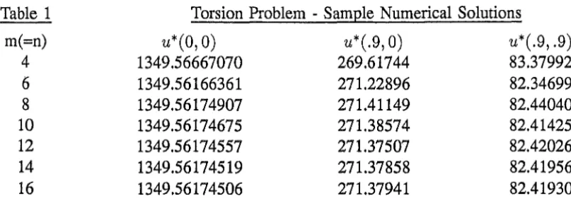
Example 1. Torsion Problem

Consider first a standard torsion problem, with no 8 term and constant _I and

f

terms, namely

1 = .5625, 8 = 0,

f

= 3600 in (3.1).

This corresponds, after transformation to the square -1

:S

x, y :::;; 1, to the Poisson problem

Table 1 m(=n)

4

6

8 10 12 14 16

Torsion Problem - Sample Numerical Solutions

u*(O,

0)

1349 .56667070 1349.56166361 1349.56174907 1349.56174675 1349.56174557 1349.56174519 1349.56174506

u*(.9,0)

269.61744 271.22896 271.41149 271.38574 271.37507 271.37858 271.37941

u*(.9,

.9)

83.37992 82.34699 82.44040 82.41425 82.42026 82.41956 82.41930

In Table 2 we give the computed Chebyshev series coefficients Cij for m=n=4, which define the

approximate solution

u*

in the form (5.3).

Table 2 Torsion Problem - Chebyshev Series Coefficients : m=n=4

en

.18027938 x 104 c31 .62316317 x102

Cl2 .48073771 x 103 c32 .10627902 x 103

c13 .10009029 x 103 c33 .63997927 x 102

Cl4 .29627816 x102 · c34 .26766070 x 102

c21 .31705951 x 103 c41 .11473890 x 102

c22 .37866829 x 103 c42 .20675183 x 102

c23 .14930920 x 103 C43 .14517153 x 102

c24 .49836904 x 102 c44 .69583688 x 101

Example 2. Torsion with Variable Coefficients

For this problem, 8 is again taken to be zero, but

,(y)

is allowed to vary with

y;

specifically we consider the case

The results

u*

obtained for this problem at the sample points are given in Table 3 and it is clear that at

(0, 0), (.9, 0)

and

(.9, .9)

the solution is correct to 7-9 decimal places for m=n=16. High accuracy has again been achieved.

Table 3 Torsion With Variable Coefficients - Sample Solutions

m(=n)

u*(O,

0)

u*(.9,

0)

u*(.9,

.9)

4 .66330955411 .13454191413 .051612213

6 .66386936129 .13688050186 .049780573

8 .66387856009 .13723959239 .049970897

10 .66387878560 .13725129342 .049955295

12 .66387879786 .13724333440 .049962553

14 .66387879977 .13724505733 .049962609

[image:12.598.86.490.77.219.2]

Example 3. Confined Aquifer Problem

Consider the steady state flow in a confined aquifer, given by the equation (3.4 ), corre-sponding to the specific · case

1

= (1 -

!

y2)2, 8

=

11(y),

f

=

exp (x 2 - y2) in

(3.1),

namely

8

2u

8 [ (

1 2) 2 au

l (

2 2)

8x2

+

8y 1 - 2 y 8y

+

exp x - y = 0 .

The results

u*

at

(0, 0), (.9, 0)

and

(.9, .9)

are given in Table

4,

and, in this case, fairly uniform results of about 5-6 decimal places of accuracy are achieved for m=n=lO.

Table 4

m(=n)

4

6

8 10

Steady State Flow in a ~onfined Aquifer - Sample Solutions

u*(O,

0)

u*(.9,

0)

u*(.9,

.9)

.389807095 .09631361 .03300478 .391141736 .09811100 .03190094 .391173149 .09835505 .03202999 .391173991 .09836919 .03202387

In Table 5 are given the computed Chebyshev series coefficients Cij for m=n=4.

Table

5

Steady State Flow in a Confined Aquifer - Chebyshev Coefficients m=n=4

en

.67575820 x 100 c:n .27246550 x 10-l ci2 .27653375 x 100 c32 .41748915 x10- 1

c13 .93330349 x 10-l c33 .29633952 x 10-l C14 .31186375 x10-1 c34 .14365799 x 10-1 c21 .17025069 x 100 c41 .46038077 x 10-2 c22 .14565509 x 100 C42 .81336266 x 10-2

c23 .83935323 x 10-1 C43 .60895092 x 10-2 c24 .35627641 x 10-l c44 .31358589 x 10-2

7. CONCLUSIONS

(i) The collocation-series method, based on approximation in the Chebyshev polynomial form

(5.3), has yielded numerical solutions of high accuracy.

(ii) The method is applicable and has good numerical properties for relatively large degrees m and n in the form of approximation.

(iii) The method requires only O(n4) operations (where mis proportional ton) and is therefore relatively efficient.

(iv) Although it is in principle possible to reduce the operation count in the method to O(n3), this has not yet been achieved without sacrificing numerical stability. The challenge therefore remains to adapt the algorithm into (a stable) one with only O(n3) operations.

[image:13.604.89.517.394.538.2]

ACKNOWLEDGEMENTS

We sincerely thank Dr R.S.Anderssen (CSIRO, Canberra) and Dr A.R. Davies (University of Aberystwyth), the organisers of this Mini-Symposiu!ll, for their encouragement and patience, and we are grateful also to Dr

A.

McNabb (Massey University, N.Z.) for his advice on relevant applications. We acknowledge the academic support of the Mathematics Departments at RMCS (Cranfield) Shrivenham, Australian Defence Force Academy (University of New South Wales), and University of Canterbury, and of the Centre for Mathematical Analysis at Australian National University.

REFERENCES

[1] C. CANUTO, M.Y. HUSSAINI, A. QUARTERONI, and T. ZANG,

Spectral Methods in

Fluid Dynamics,

Springer Verlag, Berlin, 1988.

[2] D.B. HAID VOGEL and T. ZANG,

The accurate solution of Poisson's equation by

expan-sion in Chebyshev polynomials,

J. Comp. Phys. 30 (1979), 167-180.

[3] J.C. MASON,

Chebyshev polynomial approximations/or the L-membrane eigenvalue

problem,

SIAM J. Appl. Math.

15

(1967), 172-186.

[4] J.C. MASON,

Some properties and applications of Chebyshev polynomial and rational

approximation.

In "Rational Approximation and Interpolation", P.R. Graves-Morris, E.B. Saff and R.S. Varga (Eds.), Springer Verlag, Berlin, (1984), 27-48.

[5] J.C. MASON and 0.0. OLAOFE,

Vector collocation - tau .method for linear partial

differential equations,

Math. Comput. Modelling

11

(1988), 656-660.

[6] C. LANCZOS,

Applied Analysis,

Prentice Hall (1956). .

[7] C.W. CLENSHAW,

The numerical solution of linear differential equations in Chebyshev

series,

Proc. Camb. Phil. Soc. 53 (1957), 134-149.

Applied and Computational Mathematics Group Royal Military College of Science

Shrivenham Swindon Wiltshire SN68LA ENGLAND

Department of Mathematics University of Canterbury Christchurch

NEW ZEALAND