On the Generalization of Integrator and Integral Control Action

http://dx.doi.org/10.4236/ijmnta.2014.32007

On the Generalization of Integrator and

Integral Control Action

Baishun Liu

Academy of Naval Submarine, Qingdao, China Email: baishunliu@163.com

Received 16 April 2014; revised 16 May 2014; accepted 23 May 2014

Copyright © 2014 by author and Scientific Research Publishing Inc.

This work is licensed under the Creative Commons Attribution International License (CC BY). http://creativecommons.org/licenses/by/4.0/

Abstract

This paper provides a solution to generalize the integrator and the integral control action. It is achieved by defining two function sets to generalize the integrator and the integral control action, respectively, resorting to a stabilizing controller and adopting Lyapunov method to analyze the stability of the closed-loop system. By originating a powerful Lyapunov function, a universal theo-rem to ensure regionally as well as semi-globally asymptotic stability is established by some bounded information. Consequently, the justification of two propositions on the generalization of integrator and integral control action is verified. Moreover, the conditions used to define the func-tion sets can be viewed as a class of sufficient condifunc-tions to design the integrator and the integral control action, respectively.

Keywords

General Integral Control, Nonlinear Control, General Integrator, General Integral Action, Sufficient Condition, Lyapunov Function, Output Regulation

1. Introduction

most appropriate integrator and integral control action to design their own integral controller. As a result, it also leads to a challenging trouble because the stability of the closed-loop system depends on not only the uncertain parameters and the unknown disturbances but also the general integrator and integral control action.

1.1. Traditional Integrator and Integral Control Action

Before the idea of general integral control appeared, all of the integrators were called the traditional integrator. Thus, traditional integrators can be classified into four kinds of integrators: 1) the simplest integrator, which is achieved by integrating the error; 2) the conditional integrator [2]-[7], in which the integrator value is frozen or restricted when certain conditions are verified; 3) the back-calculation integrator [8]-[11], in which the differ-ence between the controller output and the actual plant input is fed back to the integrator; 4) the nonlinear inte-grator [12]-[16], whose output is shaped by a nonlinear error function before it enters the integrator. In addition, a class of special conditional integrator was proposed by [7], in which the integrator was shaped by integrating the linear combination of the error and its derivative, but its value can be changed only inside the boundary layer. All these integrators, except for the one proposed by [7], were designed by using the error as the indispensable element. All these traditional integral control actions are almost shaped by multiplying the output of the integra-tor by a gain coefficient.

1.2. General Integrator and Integral Control Action

In 2009, the idea of general integral control, which uses all available state variables to design the integrator, was proposed by [17], where presented some linear and nonlinear general integrators. However, their justification was not proved by strictly mathematical analysis. In 2012, the rationality of the linear integrator [18] on all the states of the system was proved by using linear system theory. The results, however, were local. The regionally as well as semi-globally results were proposed in [19], where the sliding mode manifold was used as the inte-grator, and then general integral control design was achieved by using sliding mode technique and linear system theory. In 2013, based on feedback linearization technique, a class of nonlinear integrator, which was shaped by a linear combination of the diffeomorphism, was presented by [20]. General concave function gain integrator was proposed in [21], where the partial derivative of Lyapunov function was introduced into the integrator. General convex function gain integrator was presented in [22], where a systematic method to construct the con-vex function gain integrator, whose output is bounded in time domain, was proposed. Except for general concon-vex and concave integral control, all the general integral control actions above are shaped by multiplying the output of the integrator by a gain coefficient. However, the integral control actions of general convex and concave integral control are generalized by two function sets, respectively, and the indispensable element used to design the concave and convex function gain integrators is only extended to the partial derivative of Lyapunov func-tion.

All these integrators along with the integral control actions above constitute only a minute portion of the inte-grators and the integral control actions, and therefore lack generalization. Moreover, in consideration of the complexity of nonlinear system, it is clear that we cannot expect that a particular integrator or a particular integral control action has the high control performance for all nonlinear system. For these reasons above, the generalization of the integrator and the integral control action appears naturally because for all nonlinear system, we cannot enumerate all the categories of the integrators and the integral control actions with high control per-formance. It is not hard to know that this is a very valuable and challenging problem and the new theorem could be needed to solve this trouble.

to ensure regionally as well as semi-globally asymptotic stability is established by some bounded information. Consequently, the justification of two propositions on the generalization of the integrator and the integral control action is verified. Moreover, Lyapunov function proposed here has an important significant, and even could lay the foundation of the stability analysis of the complex nonlinear system with general integral control.

Throughout this paper, we use the notation λm

( )

A and λM

( )

A to indicate the smallest and the largest

ei-genvalues, respectively, of a symmetric positive-define bounded matrix A x

( )

, for any x∈Rn. The norm of vector x is defined as x = x xT , and that of matrix A is defined as the corresponding induced norm

( )

T

M

A = λ A A .

The remainder of the paper is organized as follows: Section 2 describes the system under consideration, as-sumption and definition; Section 3 addresses the method to generalize the integrator and the integral control ac-tion. Conclusions are presented in Section 4.

2. Problem Formulation

Consider the following nonlinear system,

(

)

(

)

(

)

, ,

,

x f x w g x w u

y h x w

 = +

  = 



(1)

where n

x∈R is the state, m

u∈R is the control input, y∈Rm is the controlled output, l

w∈R is a vector of unknown constant parameters and disturbance. The function f, g and h are continuous in

(

x w u, ,

)

on the con-trol domain Dx×Du×Dw⊂Rn×Rm×Rl. In this study, the function f x w

(

,

)

does not necessarily vanish at

the origin; i.e., f

(

0,w

)

≠0. Let r∈Dr⊂Rm be a vector of constant reference. Set ϑ≡

( )

r w, ∈Dϑ and

r w

D_ϑ ≡D ×D . We want to design a feedback control law u such that y t

( )

→r as t→ ∞.

Assumption 1: For each ϑ ∈D_ϑ, there is a unique pair

(

x u0, 0

)

that depends continuously on ϑ and

satis-fies the equations,

(

)

(

)

(

)

0 0 0

0

0 , ,

,

f x w g x w u

y r h x w

 = +

  = =

 (2)

so that x0 is the desired equilibrium point and u0 is the steady-state control that is needed to maintain

equili-brium at x0, where y=r.

For convenience, we state all definitions, assumptions and theorems for the case when the equilibrium point is at the origin of _Rn

, that is, x0 =0.

Assumption 2: No loss of generality, suppose that the function g x w

(

,

)

satisfies the following inequalities,

(

,

)

0

M m

g ≥g x w ≥g > (3)

(

,

)

(

0,

)

_gx

g x w −g w ≤l x (4)

for all x∈Dx and w∈Dw. where x g

l is a positive constant.

Assumption 3: Suppose there is a control law ux

( )

x such that the inequality (5) holds and x=0 is an

ex-ponentially stable equilibrium point of the system (6),

(

,

)

(

0,

)

(

,

) ( )

x

x f

f x w − f w +g x w u x ≤l x (5)

(

,

)

(

0,

) (

,

) ( )

x

x= f x w − f w +g x w u x (6) and there exists a Lyapunov function Vx

( )

x such that the following inequalities,

( )

2 2

1 x 2

c x ≤V x ≤c x (7)

( )

4

x

V x

c x x

∂

≤

∂ (8)

( ) ( ) ( ) ( ) ( )

(

)

2

3

, 0, ,

x

x

V x

f x w f w g x w u x c x

x

∂

− + ≤ −

hold for all x∈Dx, w∈Dw, where x f

l , c1, c2, c3 and c4 are all positive constants.

Definition 1: F a b c x_φ

(

_φ, _φ, _φ,

)

with a_φ >0, b_φ >0, c_φ >0 and x∈Rn denotes the set of all continuous differential increasing functions,

( )

( )

( )

( )

T

1 1 2 2 n n

x x x x

φ _{= }φ φ  φ _ such that

( )

0 0

φ = ,

( )

i xi bφ

φ ≥ ∀ ∈xi R x: i >aφ

( )

d i i d i 0

c_φ ≥ φ x x > ∀ ∈xi R

(

i=1, 2,,n

)

.

where • stands for the absolute value.

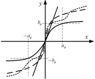
Figure 1 depicts the example curves of one component of the functions belonging to the function set Fφ. For instance, for all x∈R, the functions, ax a

(

>0

)

, tanh

( )

x , arcsinh x

( )

and so on, all belong to function set

Fφ.

Definition 2: F c xv

(

v,

)

with cv >0 and

n x

x∈D ⊂R denotes the set of all integrable function v x

( )

such that

( )

( )

1 2 n

v v v

v x z x

x x x

∂ ∂ ∂ 

= _{∂ ∂ ∂} 

   ,

( )

0

v i

v

c z

x

∂ ≥ >

∂ , i=1, 2,,n.

where z is a point on the line segment connecting x to the origin.

Figure 2 depicts the example curves of one component of the functions belonging to the function set Fv. For

instance, for all x1∈ −

(

1,1

)

, x2∈ −

(

1,1

)

, and x3∈ −

(

1,1

)

, the functions, 1 2 2 3 2

x + x + x , tanh

(

x1+2x2

)

+sinh

( )

x3 ,

(

1 2 3

)

sinh x +3x +x , tanh

(

x1+2x2+3x3

)

,

(

)

( )

(

1 2 3

)

sinh 3 tanh x +2x +2 sinh 3x ,

(

)

5

1 2 3 1 2 3

x +x +x + x +x +x

and so on, all belong to the function set Fv.

Discussion 1: The condition for Definition 2 is induced by mean value theorem. It seems to be difficulty to construct such a multivariable function, in fact, it can be designed by the following method: for each component of x, we can design a single variable function v xi

( )

i , which satisfies the conditions of Definition 2, such as

(

0

)

i

ax a> , tanh

( )

xi , sinh

( )

xi ,

(

)

2 1

1, 2,

n

i i

x +x + n=  , the functions shown in Figure 2 and so on, and then the function v x

( )

can be created by using these single variable functions v xi

( )

i , such as

( )

1

( )

1 2

( )

2 n

( )

n

v x =v x +v x + + v x ,

( )

tanh

(

1

( )

1 2

( )

2 n

( )

n

)

v x = v x +v x + + v x ,

( )

sinh

(

1

( )

1 2

( )

2

)

tanh

(

3

( )

3 n

( )

n

)

v x = v x +v x + v x + + v x ,

and so on.

3. Generalization Method

In general, integral controller comprises three components: the stabilizing controller, the integral control action and the integrator. Therefore, for achieving the generalization of the integral control action and the integrator, we resort to the control law ux

( )

x given by Assumption 3 as the stabilizing controller, and then the integral

[image:5.595.172.489.77.488.2]

Figure 1. Example curves of one component of the functions belonging to the function set Fφ.

Figure 2. Example curves of one component of the functions belonging to the function set Fv.

( )

( )

( )

x

u u x K

v x

σφ σ

σ

 = −

  =

 (10)

where K_σ is a positive-define diagonal matrix; the functions φ

( )

• and v

( )

• belong to the function sets Fφ and Fv, respectively.

Thus, substituting (10) into (1), obtain the augmented system,

(

)

(

) ( )

(

)

( )

, , _x ,

x f x w g x w u x g x w K

v x

σσ

σ

 = + −

  = 



 (11)

By Assumption 1 and choosing K_σ to be nonsingular and large enough, and then setting x=0 and x=0

of the Equation (11), we obtain,

(

0,

)

( )

0

(

0,

)

g w Kσφ σ = f w (12) Therefore, we ensure that there is a unique solution σ0, and then

(

0,σ0

)

is a unique equilibrium point of

the closed-loop system (11) in the domain of interest. At the equilibrium point, y=r, irrespective of the value of w.

Now, the design task is to provide the conditions on the control parameters such that

(

0,σ0

)

is an

asymptot-ically stable equilibrium point of the closed-loop system (11) in the control domain of interest, which is not a trivial task because the closed-loop system depends on not only the unknown vector w but also two general functions φ

( )

• and v

( )

• . This needs to establish a universal theorem.

Theorem 1: Under Assumptions 1 - 3, if there exists a positive-define diagonal matrix Kσ such that the fol-lowing inequality,

( )

(

)

(

0,

)

m g Km σ aφ f w

[image:5.595.234.393.86.217.2]

and the inequality (20) hold, and then

(

0,σ0

)

is an exponentially stable equilibrium point of the closed-loop

system (11). Moreover, if all assumptions hold globally, and then it is globally exponentially stable. Proof: To carry out the stability analysis, we consider the following Lyapunov function candidate,

( ) ( )

(

)

( )

T

0

, _{x z}

V xφ σ −φ σ =V x +z P z (14) where 12 21 x z P P P

P Pσ

 

=  

 ,

( ) ( )

0

x z

φ σ φ σ

 

=  ₋ 

 ,

z

P is a positive-define

(

n+m

) (

× +n m

)

matrix;

x

P is a n n× matrix; P_σ is a m m× matrix;

12

P is a n m× matrix, P12 =P21T, P g K12 m σ >0.

Obviously, Lyapunov function candidate (14) is positive-define. Therefore, our task is to show that its time derivative along the trajectories of the closed-loop system (11) is negative define, which is given by,

( ) ( )

(

)

( )

( )

( )

(

( ) ( )

)

( )

(

( ) ( )

)

( )

( ) ( )

(

)

(

( ) ( )

)

T T 0 T T 21 0 T T 12 0 T T

12 0 0 21

, x x x

V x

V x x x P x x P x

x

P x P

x P P

x P P x

σ

σ

φ σ φ σ

φ σ φ σ φ σ φ σ φ σ φ σ φ σ φ σ

φ σ φ σ φ σ φ σ ∂ − = + + ∂ + + − + + − + − + −  _{  }       (15)

By using (12), the closed-loop system (11) can be rewritten as,

(

)

(

) ( ) (

)

( )

(

)

(

)

(

) ( )

(

)

(

( ) ( )

)

(

) (

)

(

)

( )

0 0 , , ,

, 0, ,

,

, 0,

x

x

x f x w g x w u x g x w K

f x w f w g x w u x

g x w K

g x w g w K

σ

σ

σ

φ σ

φ σ φ σ φ σ = + − = − + − − − −  (16)

By Definition 2, we have,

( )

x

v

v x ≤l x

(

l_vx >0

)

∀ ∈x Dx

and then, using Definition 1, obtain,

( )

(

d

( )

d

)

c l_φvx x x D_x

φ σ = φ σ σ σ ≤ ∀ ∈ (16)

Substituting (16) into (15), and using (3), (4), (5), (8), (9) and (16), we have,

( ) ( )

(

)

2

( ) ( )

( ) ( )

2

0 0 0

, _xx _x

V x φ σ −φ σ ≤ −ρ x +ρσ x φ σ −φ σ −ρ φ σ_σσ −φ σ (17) where

(

) (

)

(

)

3 4 2 12 21

x x f x x f x x f

x c c lg g Px lf lg g c lφv lg g P P

ρ = − γ − + γ − + γ + ,

(

4 2

)

2

(

12 21

)

x x

x c Px g KM c lv P lf P P

σ

σ φ σ

ρ = + + + + ,

(

)

(

T

)

(

)

12 21

m g Km P m P g Km

σ

σ σ σ

ρ =λ +λ

and

(

0,

) (

0,

)

f

g f w g w

γ ≥ .

and then inequality (17) can be rewritten as,

( ) ( )

(

)

T

0

,

where

( ) ( )

0

x

η= _{φ σ −φ σ} 

 

 ,

0.5 0.5

x

x x

x

Q

σ

σ σ

σ

ρ ρ

ρ ρ

 − 

=  

−

 .

The right-hand side of the inequality (18) is a quadratic form, which is negative define when,

0.25 0

x

x x x

σ σ σ

σ

ρ ρ − ρ ρ > (19) Using the fact that Lyapunov function (14) is a positive-define function and its time derivative is a negative define function if the inequalities (13) and (20) hold, we conclude that the closed-loop system (11) is stable. In fact, V=0 means x=0 and σ σ= 0. By invoking LaSalle’s invariance principle [23], it is easy to know

that the closed-loop system (11) is asymptotically stable.

Discussion 2: Although Theorem 1 is proved by resorting to a stabilizing controller ux

( )

x along with a

Lyapunov function Vx

( )

x , the rationality of the integrator and the integral control action in (10) still can be

ve-rified because the stabilizing controller can be designed by using linear system theory, feedback linearization technique by taking the diffeomorphism as the variable of v

( )

• , sliding mode technique by taking the sliding mode manifold as the variable of v

( )

• and so on. Therefore, the justification of the following two propositions can be verified.

Proposition 1: The integrator can be taken as any integrable function, which passes through the origin and whose partial derivative, induced by mean value theorem, is positive-define and bounded. Moreover, the condi-tions on the function above can be viewed as a class of sufficient condicondi-tions to design an integrator.

Proposition 2: The integral control action can be taken as any continuous differential increasing function with the positive-define bounded derivative. Moreover, the conditions on the function above can be viewed as a class of sufficient conditions to design an integral control action.

Discussion 3: Compared with the integrators and the integral control actions proposed by [1]-[23], it is ob-vious that: 1) the integrator is not confined to the several forms and can be taken any function, which belongs to the function set Fv; 2) the integral control action is not confined to the several forms, too, and can be taken as

any function, which belongs to the function set F_φ. Moreover, there is great freedom in the choice of ux

( )

x

and Vx

( )

x such that for a particular application, the engineers can choose the most appropriate stabilizing

con-troller, integrator and integral control action to design their own integral controller.

Discussion 4: From the stability analysis procedure above, it is obvious that: 1) Lyapunov function plays the most key role in the stability analysis because it is the start point and the foundation of Lyapunov method; 2) just Lyapunov function (14) is founded, and then the theorem to ensure regionally as well as semiglobally asymptotic stability is established. Therefore, two propositions can be verified; 3) just the time derivatives of Lyapunov function (14) can be transformed into a quadratic form, and then the very tedious trouble, that is, how deal with the coupling terms on x and φ σ

( )

−φ σ

( )

0 , is solved; 4) just Lyapunov function (14) is shaped by

ad-dition of a class of general Lyapunov function and a positive-define quadratic function, and then it can be used to solve the wider problem of the stability analysis of the integral control system. Moreover, it is well known that it is very difficult to find such a powerful Lyapunov function because there is no systematic method for finding Lyapunov function, which is basically a matter of trial and error. Therefore, in consideration of these reasons above and the universality of Lyapunov method, it is easy to know that Lyapunov function proposed here not only lays the foundation of the stability analysis of this paper but also could become the foundation of the stability analysis of the complex nonlinear system with general integral control.

4. Conclusions

with the positive-define bounded derivative. Moreover, the conditions on the function above can be viewed as a class of sufficient conditions to design the integral control action; 4) by originating a powerful Lyapunov func-tion, a universal theorem to ensure regionally as well as semi-globally asymptotic stability is established by some bounded information. Consequently, the justification of two propositions on the generalization of the inte-grator and the integral control action is verified. Moreover, Lyapunov function proposed here has an important significant, and even could lay the foundation of the stability analysis of the complex nonlinear system with general integral control.

References

[1] Khalil, H.K. (2000) Universal Integral Controllers for Minimum-Phase Nonlinear Systems. IEEE Transactions on Au-tomatic Control, 45, 490-494. http://dx.doi.org/10.1109/9.847730

[2] Krikelis, N.J. and Barkas, S.K. (1984) Design of Tracking Systems Subject to Actuator Saturation and Integrator Win-dup. International Journal of Control, 39, 667-682. http://dx.doi.org/10.1080/00207178408933196

[3] Hanus, R., Kinnaert, M. and Henrotte, J.L. (1987) Conditioning Technique, a General Anti-Windup and Bumpless Transfer Method. Automatica, 23, 729-739. http://dx.doi.org/10.1016/0005-1098(87)90029-X

[4] Peng, Y., Varanceic, D. and Hanus, R. (1996) Anti-Windup, Bumpless, and Conditioned Transfer Techniques for PID Controllers. IEEE Control Systems Magazine, 16, 48-57. http://dx.doi.org/10.1109/37.526915

[5] Cao, Y.Y., Lin, Z.L. and David, G.W. (2004) Anti-Windup Design of Output Tracking Systems Subject to Actuator Saturation and Constant Disturbances. Automatica, 40, 1221-1228. http://dx.doi.org/10.1016/j.automatica.2004.02.012

[6] Marchand, N. and Hably, A. (2005) Global Stabilization of Multiple Integrators with Bounded Controls. Automatica,

41, 2147-2152. http://dx.doi.org/10.1016/j.automatica.2005.07.004

[7] Seshagiri, S. and Khalil, H.K. (2005) Robust Output Feedback Regulation of Minimum-Phase Nonlinear Systems Us-ing Conditional Integrators. Automatica, 41, 43-54.

[8] Åstrom, K.J. and Rundquist, L. (1989) Integrator Windup and How to Avoid It. Proceedings of the 1989 American Control Conference, Pittsburgh, 21-23 June 1989, 1693-1698.

[9] Shahruz, S.M. and Schwartz, A.L. (1994) Design and Optimal Tuning of Nonlinear PI Compensators. Journal of Op-timization Theory and Applications, 83, 181-198. http://dx.doi.org/10.1007/BF02191768

[10] Hodel, A.S. and Hall, C.E. (2001) Variable-Structure PID Control to Prevent Integrator Windup. IEEE Transactions on Industrial Electronics, 48, 442-451. http://dx.doi.org/10.1109/41.915424

[11] Matsuda, Y. and Ohse, N. (2006) An Approach to Synthesis of Low Order Dynamic Anti-Windup Compensations for Multivariable PID Control Systems with Input Saturation. Proceedings of the 2006 Joint SICE-ICASE Conference, Busan, 18-21 October 2006, 988-993. http://dx.doi.org/10.1109/SICE.2006.315736

[12] Shahruz, S.M. and Schwartz, A.L. (1997) Nonlinear PI Compensators That Achieve High Performance. Journal of Dynamic Systems, Measurement and Control, 11, 105-110. http://dx.doi.org/10.1115/1.2801198

[13] Kelly, R. (1998) Global Positioning of Robotic Manipulators via PD Control plus a Class of Nonlinear Integral Actions.

IEEE Transactions on Automatic Control, 43, 934-938. http://dx.doi.org/10.1109/9.701091

[14] Tarbouriech, S., Pittet, C. and Burgat, C. (2000) Output Tracking Problem for Systems with Input Saturations via Non-linear Integrating Actions. International Journal of Robust and Nonlinear Control, 10, 489-512.

http://dx.doi.org/10.1002/(SICI)1099-1239(200005)10:6<489::AID-RNC489>3.0.CO;2-D

[15] Hu, B.G. (2006) A Study on Nnonlinear PID Controllers—Proportional Component Approach. Acta Automatica Sinica,

32, 219-227.

[16] Huang, C.Q., Peng, X.F. and Wang, J.P. (2008) Robust Nonlinear PID Controllers for Anti-Windup Design of Robot Manipulators with an Uncertain Jacobian Matrix. Acta Automatica Sinica, 34, 1113-1121.

http://dx.doi.org/10.3724/SP.J.1004.2008.01113

[17] Liu, B.S. and Tian, B.L. (2009) General Integral Control. Proceedings of the International Conference on Advanced Computer Control, Singapore, 22-24 January 2009, 136-143.

[18] Liu, B.S. and Tian, B.L. (2012) General Integral Control Design Based on Linear System Theory. Proceedings of the

3rd International Conference on Mechanic Automation and Control Engineering, 5, 3174-3177.

[19] Liu, B.S. and Tian, B.L. (2012) General Integral Control Design Based on Sliding Mode Technique. Proceedings of the

3rd International Conference on Mechanic Automation and Control Engineering, 5, 3178-3181.

[20] Liu, B.S., Li, J.H. and Luo, X.Q. (2014) General Integral Control Design via Feedback Linearization. Intelligent Con-trol and Automation, 5, 19-23. http://dx.doi.org/10.4236/ica.2014.51003

356-361. http://dx.doi.org/10.4236/ica.2013.44042

[22] Liu, B.S., Luo, X.Q. and Li, J.H. (2014) General Convex Integral Control. International Journal of Automation and Computing, Accepted.