Face Recognition using Two-dimensional Subspace
Analysis and PNN
BENOUIS MOHAMED Departement of informatique
&mathematique University of Oran
Algeria
tlmesani Redwan,Ph.D INTTIC,Oran
Algeria
Senouci Mohamed,Ph.D Departement of informatique
&mathematique University of Oran
ABSTRACT
In this paper, we present an new approach to face recognition based on the combination of feature extraction methods, such as two-dimensional DWT-2DPCA and DWT-2DLDA, with a probabilistic neural networks. This later is used to classify the features matrix extracts for space data created by Two-dimensional Subspace Analysis .The technique 2D-DWT is used to eliminate the illumination ,noise and redundancy of face in order to reduce calculations of the probabilistic neural network operations ,and improve a face recognition system in accuracy and computation time. The proposed approach is tested on ORL and FEI face databases. Experimental results on this databases demonstrated the effectiveness of the proposed approach for face recognition with high accuracy compared with previous methods..
Keywords
biometric, face recognition, 2DPCA, 2DLDA, DWT, PNN,DCT
1.
INTRODUCTION
The security of persons is one the major concerns of today's society. Face recognition is one the most commonly used solutions to perform automatic identification of persons. However, automatic face recognition should consider several factors that contribute to the complexity of this task i.e. occultation, changes in lighting, pose, expression and structural components (hair, beard, glasses, etc.).
Several techniques have been proposed in the past to solve the problem of face recognition. Each of them has their strengths and weaknesses, which in most cases depend on the conditions of acquiring information. Recently several efforts and research in this area attributed to increases in the performance in face recognition systems by methods known in the field of pattern recognition such as support vector matching (SVM), Markov hidden model (HMM), methods of probabilities (Bayesian networks) and artificial neural networks[1]. This latter has attracted researchers because its effectiveness in detection and classification shapes which have recently been adopted in face recognition system.
2.
The face recognition system
A face recognition system is a system for the identification and verification of individuals, which checks if a person belongs to the database, and identifies whether this is the case. The methods used in face recognition based on 2D faces are divided into three categories[2]: global methods, local methods and hybrid methods.
Approaches to facial features, local features, or analytical. This type is to apply transformations in specific locations of the image, most frequently around feature points (corners of the eyes, mouth, nose ...). They therefore require a priori knowledge of the images.
Global approaches use the entire surface of the face as a source of information without considering the local characteristics such as eyes, mouth, etc.
Hybrid methods are used to combine the advantages of global and local methods by combining the detection of geometrical characteristics (or structural) with the extraction of characteristics of local appearance.
In this paper we are interested in methods of facial feature extractions in two dimensional images which preserves the original shape of the face in a 2D matrix compared with methods of one dimensional images which represent a face by a vector. This passage matrix to vector losses some geometric and temporal information related to the pixels of the image.
2.1 Principal approach of two-dimensional
component analyses (2DPCA)
Proposed by Yang in 2004 [3], 2DPCA is the same method of feature extraction and dimensionality reduction based on Principal Component Analysis (PCA), but deals directly with facial images as matrices without having to turn them into vectors such as the traditional global approach. The authors [4] refer that 2DPCA has high performance in terms of recognition, computation time and reconstruction of the original images compared to Fisher faces, ICA, kernel PCA and eigenfaces. However, this superiority has not been theoretically justified in their article.
A.The steps of face recognition using 2DPCA:
Step training: a training set S of N face images, the idea of this technique is to project a matrix X (n, m) via a linear transformation such that:
𝑌𝑖= 𝑋. 𝑅𝑖 (1) where 𝑌𝑖 vector principal component (n, 1) and 𝑅𝑖 is the vector base projection in size (m×1). The optimal vector 𝑅𝑖 the projection is obtained by maximizing the total variance criterion generalized
𝐺𝑡=𝑀1 𝑋𝑗 − 𝑋 𝑇
(𝑋𝑗 𝑀
𝑗 =1 − 𝑋) (3) with 𝑋𝑗: l the jéme image of the training set
𝑋 : The average face matrix of the set is:
𝑋 =𝑀1 𝑀𝑗 =1 (4) In general one optimal projection axis is not enough. We must select a set of projection axes as:
𝑅1, 𝑅2, … . . , 𝑅𝑑 = 𝑎𝑟𝑔 𝑚𝑎𝑥 𝐽 𝑅 (5) 𝑅𝑖𝑇. 𝑅𝑗 = 0, 𝑖 ≠ 𝑗, 𝑖, 𝑗 = 1, … . , 𝑑
These axes are the eigenvectors of the covariance matrix corresponding to the „d‟ largest eigenvalues. The extraction of characteristics of an image using 2DPCA is:
𝑌𝑘 = 𝑋. 𝑅𝑘 ; k=1,…... d (6) where [𝑅1, 𝑅2, … . . , 𝑅𝑑]is the projection matrix and [𝑌1, 𝑌2, … . . , 𝑌𝑑] is the features matrix of the image X.
B)Choice of the number of eigenvectors
The number of eigenvectors associated with the largest eigenvalues to be retained is a big drawback of this technique. To remedy this, several researchers have adopted different solutions to select optimal eigenvalues to remedy this problem. Nguyen recently proposed a new method named random subspace two-dimensional PCA (RS-2DPCA), which combines the 2DPCA method with the technical random subspace (RS) [4]
C)The reconstitution face image using 2DPCA
In the "eigenfaces" approach, the principal components and eigenvalues can be combined to reconstruct the face image in the same manner as in the 2DPCA[5].
In method 2DPCA, a reconstruction of the images from the features is possible. An approximation of the original image with the retained information determined by d is obtained.
𝑌𝑘 = 𝐴𝑋𝑘 (k=1,2,…d), (8) Where V= [𝑌1, 𝑌2, … . , 𝑌𝑑] et U= [𝑋1, 𝑋2, … . . , 𝑋𝑑]
V=AU (9)
Where 𝑋1 ,𝑋2 .….,𝑋𝑑 are orthonormal. Thus, it is easy to obtain the reconstructed image of A as follows:
𝐴 = 𝑉𝑈𝑇= 𝑌 𝑘 𝑑
𝑘=1 𝑋𝑘𝑇 (10)
With 𝐴 𝑘 = 𝑌𝑘𝑋𝑘𝑇 (k=1,2,…d) represents the reconstructed image of A. According to Yang et al. [4], the energy of the constructed image is focused on a small number of the first component vectors corresponding to the most important eigenvalues .
D)Step classification using Euclidean distance
Classification is performed by comparing the feature matrix of the face library members with the feature matrix of the input face image. This comparison is based on the K-nearest neighbor classifier (KNN), the distance between two characteristic matrices, 𝐵𝑖= [𝑌1 𝑖 , 𝑌2 𝑖 , … . , 𝑌𝑑 𝑖 ] and 𝐵𝑗 = [𝑌1 𝑗 , 𝑌2 𝑗 , … . , 𝑌𝑑 𝑗 ] is define by :
𝑑 𝐵𝑖, 𝐵𝑗 = 𝑌𝑘 (𝑖)
− 𝑌𝑘(𝑗 )
2 𝑑
𝑘=1 (7)
We assume that the training images are 𝐵1, 𝐵2, … … . 𝐵𝑁(where N is the total number of training images), and each image is assigned to a class 𝑃𝑘 .
We take a test image B, Si 𝑑 𝐵, 𝐵𝑙 = m𝑖𝑛𝐽𝑑(𝐵, 𝐵𝐽) and 𝐵𝑙∈ 𝑤𝑘 , compared with a threshold to decide the appropriate class of the test image (𝐵 ∈ 𝑤𝑘)
2.2 Approach 2DLDA
In 2004, Li and Yuan [6] proposed a new approach to two-dimensional LDA. The main difference between 2DLDA and the classic LDA is model of data representation. LDA classic is based on the analysis of vectors, while the algorithm 2DLDA is based on the analysis of matrix.
a)Face recognition using 2D LDA
Let X be a vector of the columns n-dimensional unitary. The main idea of this approach is to project the image as a random matrix, 𝑚 × 𝑛, on X by a linear transformation follows: 𝑌𝑖= 𝐴𝑗𝑋 (8) 𝐴𝑗:Matrix (m x n)
Y: the m-dimensional feature vector of the image A projected. on suppose L:number of classes
M: the total number of training images
The training image is represented by a matrix 𝑚 × 𝑛 𝐴𝑗(𝑗 = 1, … … . 𝑀)
𝐴 𝑖 (i=1,……L) : the mean of all classes 𝑁𝑖 : number of samples in each class
The optimal vector projection is selected as a matrix with orthonormal columns that maximize the ratio of the determinant of the dispersion matrix of the projected images to the inter-class determinant of the dispersion matrix of the
projected images intra-class:
𝐽𝐹𝐿𝐷 𝑊𝑜𝑝𝑡 = 𝑎𝑟𝑔 max𝑊 𝑊
𝑇𝑆𝑏𝑊
𝑊𝑇𝑆𝑤𝑊 (9)
𝑃𝑏=trace (𝑆𝑏) 𝑃𝑊=trace (𝑆𝑤)
where, 𝑆𝑏: the dispersion matrix inter-class, 𝑆𝑤 : the dispersion matrix intra-class 𝑆𝑏= 𝑁𝑖=1𝑁𝑖 𝑌 𝑖− 𝑌 𝑌 𝑖− 𝑌
𝑇
𝑆𝑏 = 𝑁𝑖 𝐿
𝑖=1
𝐴 𝑖− 𝐴 𝑋 𝐴 𝑖− 𝐴 𝑋 𝑇
𝑺𝑾= 𝑌 𝑘− Y 𝑌 𝑘− 𝑌 𝑇 𝒚𝒌∈𝑷𝒊
𝑳 𝒊=𝟏
𝑺𝑾= 𝐴 𝑘− 𝐴 𝑋 𝐴 𝑘− 𝐴 𝑋 𝑇 𝒚𝒌∈𝑷𝒊
𝑳
𝒊=𝟏
that means:
= 𝑋𝑇𝑆𝑏𝑋 (10) 𝑡𝑟𝑎𝑐𝑒 𝑺𝑾 = 𝑿𝑻 𝒚𝒌∈𝑷𝒊 𝐴 𝑖− 𝐴 𝑇
𝑳
𝒊=𝟏 𝐴 𝑖− 𝐴
= 𝑋𝑇𝑺𝑾𝑿 (11) The criterion can be expressed by:
𝐽 𝑋 =𝑋𝑋𝑇𝑇𝑆𝑆𝑊𝑋
𝑏𝑋 (12)
where X : column vector unitary.
The unitary vector X maximizing J (X) is called the projection axis. The optimal projection is chosen when 𝑋𝑂𝑃𝑇 maximizes the criterion, as the following equation:
𝑋𝑂𝑃𝑇= 𝑎𝑟𝑔𝑚𝑎𝑥𝑋𝐽 𝑋 (13) if 𝑆𝑊 is invertible, the solution of optimization is to solve the generalized eigenvalue problem.
𝑆𝑏𝑋𝑜𝑝𝑡= 𝜆𝑆𝑊𝑋𝑜𝑝𝑡 (14) λ is the maximum eigenvalue of 𝑆𝑊−1𝑆𝑏
In general, it is not enough to have only one optimal projection axis. We need to select a set of projection axes,𝑥1, 𝑥2, … . 𝑥𝑑 with under constraints are the following: 𝑥1, 𝑥2, … . 𝑥𝑑 = 𝑎𝑟𝑔𝑚𝑎𝑥𝑋𝐽 𝑋
𝑋𝑖𝑇𝑋𝑗 = 0, 𝑖 ≠ 𝑗, 𝑖, 𝑗 = 1,2, … . . 𝑑
Indeed, the optimal projection axes, 𝑥1, 𝑥2, … . 𝑥𝑑 are orthonormal eigenvectors of 𝑆𝑊−1𝑆𝑏 corresponding to the largest eigenvalue of the scatter matrix for creating a new projection matrix X, which is a matrix of 𝑛 × 𝑑 :
𝑋 = 𝑥1, x2, … . 𝑥𝑑
A) Feature extraction
We will use the optimal projection vectors 2DLDA 𝑥1, 𝑥2, … . 𝑥𝑑 to extract the image feature, use the following equation:
𝑦𝑘 = 𝐴𝑋𝑘, 𝑘 = 1,2, … . 𝑑 (15) Then we have a family of feature vectors 𝑦1, 𝑦2, … . 𝑦𝑑 which represent by 𝑦 = 𝑦1, 𝑦2, … . 𝑦𝑑 of size 𝑀 × 𝑑 called matrix image characteristics A.
B) Step classification using distance Euclidean
Given two face images A1, A2, represented by the feature matrix 2DLDA, is the same principle as method 2DPCA
3.
Discrete wavelet transform (DWT)
Discrete wavelet transform (DWT) is a well-known tool in the field of signal processing. It is widely used in feature extraction, compression and denoising applications. The discrete wavelet transform has been used in various studies of face recognition. The main advantage of the wavelet
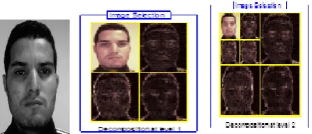
[image:3.595.318.542.71.167.2]transform over the Fourier transform is the location in time-scale. Mallat [7] shows that the discrete wavelet transform (DWT-"Discrete Wavelet Transform") may be implemented using a bank of filters including a low-pass filter (PB) and a high-pass filter (PH).
Figure 1. Wavelet decomposition at different levels (a) original image, (b) the wavelet decomposition to a single level (c) 2-level
4. Face classification using PNN
Several studies have shown improved face recognition systems using a neural classification compared to classification based on Euclidean distance measure [8]..
4.1 The neural network
[image:3.595.322.568.317.420.2]An artificial neural network is a computational model whose design is inspired by the schematic of biological neurons.
Figure 2 . Schematic representation of a neural network with a single layer standard Hidden.
4.2 probabilistic neural networks
The probability neural network is proposed by D. F. Specht for solving the problem of classification in 1988 [11]. The theoretical foundation is developed based on Bayes decision theory, and implemented in a feed-forward network architecture. The Bayesian decision theory is the principle concept of classification that uses statistical inference, mainly to find the maximum expectation of the smallest risk. The raw data are divided into C classes, which represent the C situations to be explained. Each class has m-dimensional observations, i.e.X[X1,X2, Xm]. The following Bayes decision rule is used to classify the raw data into C classes:
)
(
)
(
X
h
c
P
X
P
c
h
i i i
j j j
j
i
,where
h
Cis the prior probability of class C;M
C is the representative center that belongs to the class C, but the loss function has been a miscarriage of justice; and 𝑃𝐶 is the probability density function of class CThe probability density function for each class can be expressed as follow:
Nij
ij t ij i
d d i
x
x
x
x
N
x
P
1
2
2
2
)
(
)
(
exp
1
)
2
(
1
)
(
wherePi(x)denotes the dimension of training vector,
is the smoothing parameter and d is the dimension of training vector. 𝑁𝑖denotes the total number of training vector in categoryi
, and 𝑥𝑖𝑗is the neuron vector andx
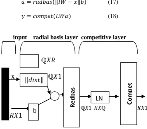
is test vector.PNN represent mathematically by the flowing expression : 𝑎 = 𝑟𝑎𝑑𝑏𝑎𝑠( 𝐼𝑊 − 𝑥 𝑏) (17)
𝑦 = 𝑐𝑜𝑚𝑝𝑒𝑡(𝐿𝑊𝛼) (18)
input radial basis layer competitive layer
ℚ𝑋𝑅
x ℚ𝑋1
y
ℚ𝑋1 𝐾𝑋ℚ 𝐾𝑋1
[image:4.595.310.556.116.609.2]𝑅𝑋1
fig 3. Architecture of a probabilistic neural networks[13] Q:number of input target/pairs :number input layers R:number of classes of input data: number output layers IW: input weight
LW: layer weight
a) The structure PNN : The PNN architecture consists of two layers[12]:
the first layer computes distances from input vector to the input weights (IW) and produces a vector whose elements indicate how close the input is to the IW .
The second layer sums these contributions for each class of inputs to produce as its net output a vector of probabilities .Finally a compete transfer function on the output of the second layer picks the maximum of these probabilities and produces a 1 for that class and a 0 for the other classes. The architecture for this system is shown above.
The probability of neural network with back propagation networks in each hidden unit can approximate any continuous nonlinear function. In this paper, we use the Gaussian function as the activation function:
radbasexp
(n2)
(19)Finally, one or many larger values are chosen as the output unit that indicates these data points are in the same class via a competition transfer function from the output of summation unit [11], i.e.
𝑐𝑜𝑚𝑝𝑒𝑡 𝑛 = 𝑒𝑖= 000 010 … . . 0𝑖 ,𝑛 𝐼 = 𝑀𝐴𝑋(𝑛)
In order to implement a face recognition system by our approach, we follow this methodology:
stage pretreatment using technique DWT
feature extraction using 2DPCA/2DLDA
[image:4.595.53.293.160.371.2] classification using PNN network
Figure 1 shows the block diagram of this approach.
face known face unknown
Figure 3. diagram of our approach applied to face recognition
For face recognition task, we applied Two-dimensional Subspace Analysis (2DPCA,2DLDA) which capable of creating the face subspace, defined as orthogonal basis of vectors that contain the most relevant information about a face. These vectors are the eigenvectors of the covariance matrix of the distribution. The recognition process is achieved by forwarding feature matrix which must be transformed into vectors before providing them to the PNN classifier to performed classification and decision.
b
𝑑𝑖𝑠𝑡
∗
Red
b
as
LN
C
o
mpe
t
Database of reference images
Pretreatment by technique DWT
Construction projection
matrix2DPCA Projection
images of tests on the projection
matrix 2DPCA
Training network PNN by weight of
projection matrices 2DPCA Face Recognition
using PNN network (Decision) Database of test images
Pretreatment by technique DWT
calculating the weight of face
images reference on
4.
Results and Discussion
In order to evaluate and test our approach described for a face recognition system, we chose three databases: ORL database, FEI and our database constructed by our laboratory. All experiments were performed on MATLAB installed on a laptop with a dual processor T5870 at 2.03 GHz and 2 GB RAM.
A) ORL database
In this database, the faces are made in an environment where the light variation is homogeneous. Different facial expressions may appear without being defined by the constructors of the base. It contains 10 different images for each of 40 people photographed. Inclinations of 20 degrees more, head to the left such as the right, may occur. These images are grayscale with a dimension of 92 * 112 pixels.
Figure 4. our images of the same person from the ORL database
B) FEI database:
Constructed between June 2005 and March 2006, the Artificial Intelligence Laboratory of the FEI in São Bernardo do Campo, São Paulo, Brazil, contains a set of face images, consisting of 14 different images for each of the 200 people photographed, with no head tilt. These images are grayscale with a dimension of 200 * 180 pixels.
Figure 5. four images of the same person from the FEI database
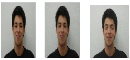
[image:5.595.310.544.224.309.2]C) Our database: We have face images collected at different times using a capture device (webcam) to form our own database. The database includes 100 face images in a JPG taken on 10 different subjects (N = 10) each registered under 10 different views.
Figure 6. five images from our database
All experiments were performed using the ORL database and FEI with 5 images for training and 5 test images per person for a total of 200 images for each phase (training and test).
A. Experience one
In this experiment we compare the performance of two approaches 2DPCA and PCA in terms of recognition rate and execution time. We use ORL database. For best results, illustrate the approach PCA and 2DPCA, fix the number of dimensions of PCA and 2DPCA, which gives better recognition rates.
After a series of experiments we choose the best values of parameters to define the choice of eigenvectors which gives a better recognition rate.
Table 1. comparison between PCA and 2D-PCA based on ORL
2DPCA PCA
recognition rate %
96.00 94.00
execution time (s) 13.718743 35.442794
Discussion:
Table (1) shows comparison between PCA and 2DPCA approaches in terms of recognition rate and execution time. We find that the recognition rate obtained by 2DPCA is better compared to that obtained with PCA.
We see that the execution time 2DPCA is less long than PCA. After these figures below, we noticed that the image
[image:5.595.63.271.264.334.2]reconstruction using approach 2D-PCA is better than the PCA whose projection error of 2D-PCA (5.05%) and fable relative to the projection error of PCA (16, 34%).
Figure 7.The reconstruction of a test image by using 2DPCA
[image:5.595.360.533.444.526.2] [image:5.595.59.276.466.529.2] [image:5.595.351.515.608.696.2] [image:5.595.56.268.633.701.2]B. Experience two
[image:6.595.43.294.165.347.2]In this experiment, we used the ORL database. The classification stage is the phase in which the system assigns a face recognition test face to one class among those of a learning base according to a certain criterion. In our experiment we use the Euclidean distance.
[image:6.595.51.275.392.577.2] [image:6.595.341.546.580.734.2]Figure 9. the recognition rate obtained by using 2D-PCA
[image:6.595.69.277.640.714.2]Figure 10. the recognition rate obtained by using 2D-LDA Table 2.: Execution time
Database FEI
Data base ORL
2DPCA(s) 21.685602 13.718743
2DLDA(s) 27.229849 20.558097
Discussion:
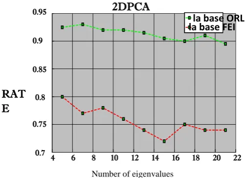
Figures (9) and (10) show the evaluation of the recognition rates based on clean faces. After a series of experiments, we observe a better recognition rate based on the seventh clean face (K = 7), which reached 94.4%. for 94.6% and 2DPCA.
From the 11th eigenvector we see a decrease in the recognition rate up to 88.4%.
The decrease in recognition rates for the two approaches is related to the phenomenon of overfitting.
C. Experience three
To evaluate the performance of our proposed approach we have tested using two databases: ORL and FEI.
a) Database: The global performance of algorithms tested on face database FEI are not as good as database ORL. There are two main reasons:
The quality of the image in the database ORL is better than the database FEI.
Database FEI is more difficult due to variations in the details of the face and head orientations. b) The stage preprocessing: We propose to add a preprocessing stage in order to improve our system in speed by reduced size and eliminating redundant information from the face images by using DWT technique.
c) Feature extraction using 2DPCA/ADLDA: After the reduction of the size of face images using DWT, we used feature extraction approaches 2DPCA and 2DLDA in order to extract the weight images, (features images in new space) which must be converted into vectors before implementing the PNN network.
d) Choice of the number of eigenvalues: Two dimensional methods do not escape this problem and the choice of the appropriate number depends on the method and the database faces used. In our experiments we have selected the best eigenvalues corresponding to the best values of variance (eigenvectors).
Figure 11. The variance of eigenvalues
4 6 8 10 12 14 16 18 20 22
0.7 0.75 0.8 0.85
0.9 0.95
Number of eigenvalues
la base ORL
la base FEI
4 6 8 10 12 14 16 18 20 22
0.7 0.75 0.8 0.85 0.9 0.95
Number of eigenvalues
la base ORL
la base FEI
RAT
E
2DPCA
RATE
e) Selection parameters and architecture PNN : our neural network training algorithm used in system face recognition is not require many parameters compared other neural networks (MLP,BP,....ex),that only parameter that is needed for performance of the network is the smoothing parameter 𝜎 .Usually, the researchers need to try different 𝜎 in a certain range to obtain one that can reach the optimum accuracy[12]. To get a higher recognition rate, we have made a series of experiments to choose the best smoothing parameter 𝜎 used in PNN .
The probabilistic Neural Network used in our system is composed of two layers:
Input layer: The first layer is the input layer and the number of hidden unit is the number of independent variables and receives the input data (number of feature extraction for each approach used in this paper)
output layer: gives the number of faces used in the Database training(ex: ORL 200 person's)
In this experiment we test the performance of face
recognition using PNN on three databases: ORL, FEI, and our database.
Table 4. The rate of face recognition by using PNN Our
data base
ORL FEI
recognition
rate 90% %88 %79
Discussion:
Table 4 shows the recognition rates obtained by using PNN on three databases. The performance of this technique decreased up to 79% when tested on FEI and long execution times.
In the last experiment, we compared the different methods described in this paper and evaluated on two databases, ORL and FEI. We followed the same protocol testing previous experiences.
we propose a stage preprocessing based technique 2DDWT to reduce affect illumination ,noise and size the databases and other hand reduce the memory of our neural network training algorithm (PNN)
In this work, it is wanted to test our system with and without added noisy in the two data base in order to evaluate robustness of these approaches namely 2DPCA, 2DLDA, DWT-2DLA, DWT-2DPCA combined by using two classifier :KNN (Euclidean distance )and PNN
[image:7.595.321.530.85.182.2]Two types of noise are used in this simulation: the Saltand Pepper type noise with a noise density a=0.06 and Gaussian noise with mean m=0, variance v=0.04 and mean m=0, variance v=0.06 .
Figure 12 illustrates these effects which are obtained as follows
(a)Salt&pepper Noise (b) Gaussian Noise (c) Gaussian Noise m=0,v=0.01 m=0, v=0.04
(a)Salt&pepper Noise (b) Gaussian Noise (c) Gaussian Noise m=0,v=0.01 m=0, v=0.04
Fig 12:Adding Noise
Table 5. The recognition rate obtained by different methods on the database ORL
Table 6. The recognition rate obtained by different methods on the database ORL with added noisy
Table 7. The recognition rate obtained by different methods on the database FEI
Type of
classifier 2DPCA 2DLDA
DWT-2DPCA
DWT-2DLDA Distance
Euclidean
94% 94 .8% 94% 95%
Network PNN
95.8 96%
97% 98%
Type classifier
2DPCA 2DLDA DWT-2DPCA
DWT-2DLDA
Distance Euclidean
90% 91% 90% 92%
Network PNN
92% 92% 94% 95%
Type of
classifier 2DPCA 2DLDA
DWT-2DPCA
DWT-2DLDA Distance
Euclidean
80% 82 .8% 90% 94%
Network PNN
88% 90%
[image:7.595.324.539.222.307.2] [image:7.595.304.549.429.503.2] [image:7.595.308.549.550.635.2] [image:7.595.309.549.688.761.2]
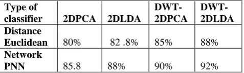
Table 8. The recognition rate obtained by different methods on the database FEI with added noisy
Discussion
:
After these series of experiments we clearly see the superiority of the two-dimensional methods combined with a probabilistic neural classifier combining those of a Euclidean distance classifier.
We also note that the choice of optimal component and the choice smoothing parameter which represents a better recognition rate for both methods, 2DPCA and 2DLDA and accuracy of classification PNN.
The results obtained after using our approach shows that it reduces the computation time of training and improves the recognition rate .
5.CONCLUSION
In this paper, we propose an approach for face recognition based on the combination two approaches, one used for the reduction of space and feature extractions in two dimensions and the other for classification and decision.
After our experience we have found clear improvement of our system, based on DWT-2DPCA and 2DLDA DWT-combined by a probabilistic neural classifier, achieved a better recognition rate compared to other techniques described in this article.
Our choice of using DWT techniques as a preprocessing stage is demonstrated by improved performance of our system in terms of recognition rate ,speed of calculation and reduce memory computation of PNN .
As a perspective, we propose to use this approach in an uncontrolled environment (video surveillance) based on video sequences (dynamic images) in order to make the task of face recognition more robust.
6. REFERENCES
[1] Handbook of Biometrics edited by Anil K. Jain Michigan State University, USA Patrick Flynn University of Notre Dame, USA Arun A. Ross West Virginia University, USA © 2008 Springer Science+Business Media, LLC. [2] biometric recognition challenges and opportunities Joseph
N. Pato and Lynette I. Millett, Editors Whither Biometrics Committee Computer Science and Telecommunications Board Division on Engineering and Physical Sciences Copyright 2010 by the National Academy of Sciences.
[3] D. Zhang and Z. -H. Zhou. (2D) 2PCA: Two-directional two-dimensional PCA for efficient face representation and recognition. Neuro computing, Vol. 69, pp. 224-23 1, 2005.
[4] N. Nguyen, W. Liu and S. Venkatesh. Random Subspace Two-Dimensional PCA for Face Recognition. Department of Computing, Curtin University of Technology, WA 6845,
[5] Two-Dimensional PCA:A New Approach to Appearance-Based Face Representation and Recognition Jian Yang, David Zhang,. 26, NO. 1, JANUARY 2004
[6]. S. Noushath, G.H. Kumar, and P. Shivakumara. (2D)2LDA : An efficient approach for face recognition. Pattern Recognition, 39(7) :1396–1400, 2006.
.[7] B-L. Zhang, H. Zhang, and S.S. Ge. Face recognition by applying wavelet subband representation and kernel associative memory. IEEE Transactions on Neural Networks, 15(1) :166–177, 2004
[8] S. Mallat. A theory of multiresolution signal decomposition : the wavelet representation. IEEE Transactions on Pattern Analysis and Machine Intelligence, 11(7) :674–693, 1989.
[9] J.Sima. Introduction to neural networks. Technical Report. N. V-755, August 10, 1998.
[10]. Nazish, 2001. Face recognition using neural networks. Proc.IEEE INMIC 2001, pp: 277-281 (2007)
[11] M. Rizon, M.H. Firdus, P. Saad, S. Yaacob, M.R. Mamat, A.Y.M. Shakkaf, A.R. Saad, Hdesa and M. Karthigayan. Face recognition using Eigenfaces and Neural Networks. American Journal of Applied Sciences, Vol. 2, pp. 1872-1875, 2006..
[12] D. F. Specht, 1990. “Probabilistic neural network and the polynomial adaline as complementary techniques for classification” IEEE Trans. Neural Networks, 1(1): 111-121.
[13] neural network toolbox matlab User‟s Guide COPYRIGHT 1992 - 2002 by The MathWorks, Inc.
Type of
classifier 2DPCA 2DLDA
DWT-2DPCA
DWT-2DLDA Distance
Euclidean
80% 82 .8% 85% 88%
Network PNN
85.8 88%
[image:8.595.50.289.119.191.2]